Multigrid Accelerated Computation of
Ligand-Receptor Interactions under Flow Condition
Wensheng
Shen
∗, Kimberly Forsten-Williams, Michael Fannon, Changjiang Zhang, and Jun Zhang
Abstract—This paper describes a multigrid finite volume method developed to speed up the solution process for simu-lating complex biological transport phenomena. The method is applied to a model system which includes flow through a cell-lined cylindrical vessel and includes fibroblast growth factor-2 (FGF-2) within the fluid capable of binding to receptors and heparan sulfate proteoglycans (HSPGs) on the cell surface. FGF-2 transport is modeled by a convection-diffusion transport equation and interactions with cellular receptors and HSPGs are modeled through a series of biochemical reaction boundary conditions. The finite volume method was used to discretize the differential equations and the multigrid V-cycle algorithm was used to solve the discretized equations, which allows for non-uniform grid spacing and multiple levels of grids. Our work indicates that a multigrid finite volume method may allow users to investigate complex biological systems currently intractable with single-grid methods.
Index Terms—Multigrid, Finite volume, Navier-Stokes equa-tion, Fibroblast growth factor, Mass transport, Biological system.
I. INTRODUCTION
Communication between cells is achieved to a great extent by soluble molecules that are transported either by diffusion through extracellular matrices or through circulation of blood and lymph. The bioavailability of these molecules to cell surfaces is regulated by a number of factors. For example, a protein may have a unique family of cell surface receptors to which it binds. This binding will trigger a cascade of downstream signaling events in the cell. The efficiency of the binding events depends in part on the concentrations of both ligand and receptor, the intrinsic binding affinity of the molecules, and the presence of competing ligands and receptors.
Basic fibroblast growth factor (FGF-2) is the prototypical member of the family of fibroblast growth factors [14]. It has been demonstrated to be important in normal physiology This research work was funded in part by NIH under grants R01-HL086644-01.Asterisk indicates corresponding author.
W. Shen is with the Department of Computational Science, SUNY Brockport, Brockport, NY, 14420 USA e-mail: [email protected] (see http://www.cps.brockport.edu/∼shen).
K. Forsten-Williams is with the Department of Chemical Engineering, Virginia Polytechnic Institute & State University, Blacksburg, VA 24601, USA e-mail: [email protected].
M. Fannon is with the Department of Ophthalmology and Visual Sci-ence, University of Kentucky, Lexington, KY 40506 USA e-mail: [email protected].
C. Zhang is with the Department of Computer Science, University of Kentucky, Lexington, KY 40506 USA e-mail: [email protected].
J. Zhang is with the Department of Computer Science, University of Kentucky, Lexington, KY 40506 USA e-mail: [email protected] (see http://www.cs.uky.edu/∼jzhang)
and pathologies in cancer development process [4], [10]. In addition to its target cell surface tyrosine kinase receptor, FGF-2 also binds with high affinity to heparan sulfate proteoglycan (HSPG), which consists of a protein core with O-linked carbo-hydrate chains that are polymers of repeating disaccharides [6]. HSPGs are present on almost all cell surfaces and generally in much higher numbers than FGF surface receptors. FGF-2 is present in circulation and its presence in elevated levels in blood is used in clinical settings as criteria for treatment strategies such as interferon alpha therapy for infantile heman-gioma [5]. Although FGF-2 binding interactions have been the subject of a number of studies in static systems, far less is known about their behavior under flow.
The interaction between biochemical reaction and mass transfer is of particular interest for the real time analysis of biomolecules in microflow systems [13], [15]. Glaser [13] proposed a two-dimensional (2D) computer model, which was greatly simplified by assuming that the flow is parallel and the diffusion is perpendicular to the surface, to study antigen-antibody binding and mass transport in a microflow chamber. Myszka et al. [15] used a computer model similar to that of Glaser [13] to simulate the binding between soluble ligands and surface-bound receptors in a diagnostic device, BIACORE, for both transport-influenced and transport-negligible binding kinetics. A 2D convection and diffusion equation was used by Chang and Hammer [2] to investigate the effect of relative motion between two surfaces on the binding of surface-tethered reactants. We take a different approach by solving the 2D convection diffusion equation directly. In addition, a multigrid method is applied to speed up the solution process.
II. METHODS
A. Mathematical Model
A coupled nonlinear convection-diffusion-reaction model for simulating growth factor binding under flow conditions has recently been developed [11], [18] and is used here. This model can be applied to predict the time-dependent distribution of FGF-2 in a capillary with complicated binding kinetics on the tube surface.
bFGFR-HSPG dimers. Consequently, the concentration of FGF-2 in the solution is affected due to the molecular binding process.
C2
G2 T2
T2 ! ! " " # # $ $ % % & & ' ' ( ( ) ) * * + + , , -. . / / 0 0 1 1 2 2 3 3 4 4 5 5 6 6 7 7 8 8 9 9 : : ; ; < < = = > > ? ? @ @ A A B B C C D D E E F F G G H H I I JKJ JKJ LKL LKL M M N N O O P P QKQ QKQ RKR RKR SKS SKS TKT TKT U U V V W W X X Y Y Z Z [ [ \ \ ]K] ]K] ^K^ ^K^ _ _ ` `aKa aKa bKb bKb c c d d eKe eKe f f g g h h i i j j k k l l R R L P P G G C C T T C2 G2
Fig. 1. Sketch of growth factor binding to receptors and HSPGs and the formation of various compounds on the surface of a capillary. The symbols in the sketch are as follows: L=FGF-2, R=FGFR, P=HSPG, C= FGF-2-FGFR complex, G=FGF-2-HSPG complex, C2=FGF-2-FGFR dimer, G
2=FGF-2-HSPG dimer, T=FGF-2-FGFR-2=FGF-2-HSPG complex, andT2=FGF-2-FGFR-HSPG
dimer. The arrows represent velocity vectors, which are uniform in the entrance and evolve to parabolic later on.
Flows in circular pipes are modeled in axisymmetric coor-dinates. The 2D time-dependent equations for fluid mass and momentum transfer in conservative form for incompressible flow can be written as:
∂ρ ∂t +
1
r
∂(rρvr)
∂r +
∂(ρvz)
∂z = 0, (1)
∂(ρvr)
∂t +
1
r
∂(rρvrvr)
∂r − 1 r ∂ ∂r
rµ∂vr ∂r
+∂(ρvrvz)
∂z
− ∂
∂z
µ∂vr ∂z
=−∂p
∂r −µ vr
r2,
(2)
∂(ρvz)
∂t +
1
r
∂(rρvrvz)
∂r − 1 r ∂ ∂r
rµ∂vz ∂r
+∂(ρvzvz)
∂z −
∂ ∂z
µ∂vz ∂z
=−∂p
∂z,
(3)
whereρis the density,µthe dynamic viscosity,pthe dynamic
pressure, andvrandvz are velocity components in the radial
and axial directions, respectively. In the above equation set, the independent variables are time t, radial coordinater, and
axial coordinatez.
The mass of each species must be conserved. If binding or reactions occur within the fluid, the coupling of mass transport and chemical kinetics in a circular pipe can be described by the following equations:
∂(ρφi)
∂t +
1
r
∂(ρruφi)
∂r +
∂(ρvφi)
∂x = 1 r ∂ ∂r
Krr
∂(ρφi)
∂r + ∂ ∂x Kx
∂(ρφi)
∂x
+Fi(φ1...φn), 1≤i≤n,
(4) where φi is the concentration of species i, uand v are the
radial and longitudinal components of velocity,KrandKzthe
molecular diffusion coefficients, andFithe rate of change due
to kinetic transformations for each speciesi. The basic model
however has only FGF-2 within the fluid (φiis simply FGF-2)
and, thus, reactions (i.e., binding and dissociation) occur only on the capillary surface. That is to say thatFiis valid merely
on the tube surface. The reactants and products involved in the chemical kinetics include FGF-2, FGFR, HSPG, FGF-FGFR complex and its dimer, FGF-HSPG complex and its dimer, FGF-HSPG-FGFR complex and its dimer, with a total of nine species (n= 9) [11].
B. Collocated finite volume discretization
A cell-centered finite volume approach is applied to dis-cretize the partial differential equations. Eqs. (1) ∼ (4) can be re-organized in the form of convection diffusion equations and written as
∂ ∂t(ρφ) +
1
y ∂ ∂y
yρvφ−yΓ∂φ
∂y
+ ∂
∂x
ρuφ−Γ∂φ
∂x
=S,
(5) wherex andy are axial and radial coordinates,u andv are
the velocity components in the axial and radial directions, respectively. It is worth noticing that the mass conservation equation is a special case of Eq. (5) in whichφ,Γ, andS are
taken asφ= 1,Γ = 0, andS= 0.
To achieve higher order temporal accuracy, we use a quadratic backward approximation for the time derivative term. Such arrangement gives us second order temporal accuracy. Integrating Eq. (5), the corresponding finite volume equations can be derived,
3(ρφ)nP+1−4(ρφ)
n P + (ρφ)
n−1
P
∆t + (Je−Jw)
+ (Jn−Js) =SC+SPφP +Ssym,
(6)
where Je,w,n,s is the convection-diffusion flux at each of
the four interfaces of the control volume P, with Je,w =
Fe,w−De,w,Jn,s=Fn,s−Dn,s,SCandSP are the results of
source term linearization, and Ssym is the contribution from
axisymmetric coordinates, with Ssym = −Γyv2 for the
mo-mentum equation ofv. The approximation of convective flux
is critical for an accurate solution. We use a so-called deferred correction technique [8]. This technique calculate higher-order flux explicitly using values from the previous iteration. In this technique, the convective flux is written as a mixture of upwind and central differences, Fe,w = Fe,wu +λ(Fe,wc −Fe,wu )o,
whereFu
e = max((ρu)e∆rj,0.)φP + min((ρu)e∆rj,0.)φE,
Fu
w= max((ρu)w∆rj,0.)φW+ min((ρu)w∆rj,0.)φP,Fec=
(ρu)e∆rj(1−αe)φP+ (ρu)e∆rjαeφE,Fwc = (ρu)w∆rj(1−
αw)φW+(ρu)w∆rjαwφP,λis a parameter set asλ= 0∼1,
and the superscript (o) indicates taking the value from the
previous iteration, which will be taken to the right hand side and treated as a part of the source term. The same can be applied to convective flux in radial direction. The interpo-lation factors are defined as αe = xxe−xP
E−xP, αw =
xP−xw
xP−xW, αn=rrn−rP
N−rP, andαs=
rP−rs
rP−rS. The diffusion fluxes areDe=
Kxyj(φE−φP)
xE−xP ,Dw=
Kxyj(φP−φW)
xP−xW ,Dn=
Krxi(φN−φP)
rN−rP , and Ds= Krxri(φP−φS)
P−rS . The notations of spatial discretization in
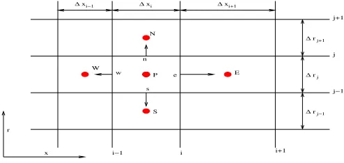
Eq. (6) is illustrated in Fig. 2, where the uppercase letters indicate the center of the control volumes, and the lowercase letters indicate the interfaces between neighboring control volumes.
Substituting numerical fluxes into Eq. (6) and collecting terms, a set of algebraic equations are obtained of the fol-lowing form
ASφS+AWφW +APφP+AEφE+ANφN =b. (7)
[image:2.612.59.302.288.423.2]∆xi−1 ∆xi ∆xi+1
∆rj+1
∆rj
∆rj−1
E N
P
S W
e n
w
s
x r
i i+1
i−1
j j+1
[image:3.612.50.297.53.170.2]j−1
Fig. 2. Finite volume notation of control volumes in axisymmetrical coordinates.
C. Multigrid methods
In finite volume method on a structured grid, the multigrid version in 2D can be constructed such that each coarse grid control volume is composed of four control volumes of the next finer grid [8]. To do this, a grid generator that is able to generate multiple grids is used. The grid generator takes input of the number of grid levels, the number of lines along each boundary, the coordinates of starting and ending points for each line, the line type, etc., for the coarsest grid. The data of the rest levels of grids are computed automatically by subdividing each control volume in finer ones and saved as binary files to be loaded by the flow solver.
In the current work, we use a full multigrid procedure previously described by Schreck and Peri´c[16]. A coarse grid
is chosen and a converged solution is obtained. This solution is interpolated to the next finer grid to obtain a starting solution. After performing a few outer iterations on the finer grid, the calculation is moved to the coarser grid, to start a V-cycle like computation.
The algebraic equation Eq. (7) can be written more ab-stractly as
Aφ=b, (8)
whereAis a square matrix,φthe unknown vector, andbthe
source vector. After the kth outer iterations on a grid with
spacing h, the intermediate solution satisfies the following
equation,
Ak
hφkh−bk=rkh, (9)
where rk
h is the residual vector after the kth iteration. Once
the approximate solution at the kth iteration is obtained, we
restrict the approximate solution as well as the residual to the the next coarse grid by the restriction operatorsI2h
h andIˆ
2h h .
An approximate solution to the coarse grid problem can be found by solving the following system of equations,
A2hφ12h=A2h(Ih2h)−Iˆ
2h h r
k
h. (10)
After the solution on the coarse grid is obtained, the correction
∆φ=φ1
2h−φ02his transfered to the fine grid by interpolation
(prolongation), whereφ0 2h=I2
h h φ
k
h. The difference ofI2 h h and
ˆ
I2h
h is as follows, Ih2h takes the mean value of states in a set
of cells, butIˆh
2h performs a summation of residuals over a set
of cells. The value of φk
h is updated by
φkh+1=φ k h+I
h
2h∆φ, (11)
where Ih
2h is a prolongation operator. This procedure is
repeated until the approximate solution on the finest grid converges using the multigrid V-cycle algorithm [16]. The relaxation technique used in the multigrid method is Stone’s strong implicit procedure (SIP), which is a modification from the standard ILU decomposition [19]. This paper has adapted the multigrid method for incompressible Navier-Stokes equa-tions provided by Schreck [16] and extended it to include the mass transport. Since the concentration of ligand is very small, in the order of 10−11 to 10−10 M, we may assume that the
momentum and mass transfer equations are independent to each other. Consequently the momentum transfer equation can be solved first to obtain the velocity distribution, which is then put into the mass transfer equation.
III. RESULTS
The flow model in the current paper is the well-known incompressible Navier-Stokes equation, which has been widely used to solve low speed fluid mechanics problems. A convection-diffusion equation is applied to address the mass transport of growth factor in solution. A similar mass transport model has been used by Glaser [13] to describe the biological interaction of antigen and antibody, and by Myszka et al. [15] to investigate the interactions of a variety of biomolecules in BIACORE, where the flow cell was of rectangular geometry. However, to study the binding and dissociation of growth factor, its receptor, and HSPG in a capillary of a cylindrical geometry with the application of a 2D Navier-Stokes equation, as far as we know, has not been reported previously. The numerical procedure and simulation results for a single grid is presented in a previous paper [18], while the main purpose of the current paper is to demonstrate a multigrid solution to the convection-diffusion-reaction model of mass transport and chemical kinetics of protein ligands.
The dimensions of the capillary under consideration were lengthL= 0.1m and radiusR= 0.00035m, corresponding
to that of a Cellmax Cartridge System bioreactor (FiberCell Systems, Inc., Frederick, MD, USA). The ratio of length over diameter is 286. To simulate the capillary flow, four types of
boundary conditions are used in the numerical simulation: inlet boundary to the left-hand side, outlet boundary to the right-hand side, symmetry boundary at the bottom, and impermeable wall boundary at the top. For inlet boundary, all quantities are prescribed, and the incoming convective flux is calculated as well. For outlet boundary, zero gradient along the grid line is applied. A three-level multigrid method is considered, and the number of control volumes are40×5,80×10, and160×20,
respectively. Each time the grid is refined, one control volume is divided into four smaller control volumes.
X
R
0 0.025 0.05 0.075 0.1
-0.0003 -0.0002 -0.0001 0 0.0001 0.0002 0.0003
0.0625 0.1875 0.3125 0.4375 0.5625 0.6875 0.8125 0.9375
(a)
X
R
0 0.025 0.05 0.075 0.1
-0.0003 -0.0002 -0.0001 0 0.0001 0.0002 0.0003
0.0625 0.1875 0.3125 0.4375 0.5625 0.6875 0.8125 0.9375
(b)
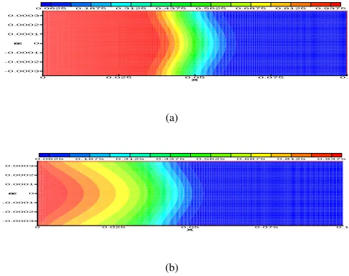
Fig. 3. A snapshot of ligand concentration distribution at t = 10minin
the capillary at the temperature of 37oCand the uniform inlet velocity of u= 5.2mm/min. (a) Surface binding is not considered. (b) Ligands bind to
receptors and HSPGs on the capillary surface.
all species are represented by a set of ordinary differential equations (ODEs), as shown in Table I, and the parameters are primarily determined by experiments [11]. The system of ordinary differential equations are solved by a variable-coefficient ODE solver VODE for stiff and nonstiff systems of initial value problems [1].
The code is developed to solve the time-dependent Navier-Stokes and convection-diffusion-reaction equations with a particular application in growth factor transport and binding. The computation is performed on a Sun-Blade-100 machine with a single 500 MHz SPARC processor and 2 GB memory. A typical numerical solution is plotted in Fig. 3, where the concentration distribution of fibroblast growth factor inside the capillary is shown at an instant time of t = 10min. The
solution in Fig. 3 corresponds to the finest grid arrangement in the multigrid system. Note that the ligand concentration in the figure is non-dimensionalized with respect to the inlet concentration on the west boundary. To demonstrate the impact of surface binding on ligand transport, two numerical exper-iments have been conducted, one without surface binding, Fig. 3(a), and the other with surface binding to receptors and heparan sulfate proteoglycans, Fig. 3(b). As expected, without surface binding, displayed in Fig. 3(a), the ligand moves with the flow by convection and diffusion, and its concentration has a uniform distribution along the radial direction in a portion of the capillary from x = 0 to roughly x = 0.05m. One
may further predict that a uniform concentration distribution in the whole capillary will be obtained after t = 20 min. It
clearly shows in Fig. 3(b) that the concentration of ligand in the capillary is spatially reduced by a great margin down along the capillary as well as in the radial direction due to biochemical reactions on the surface.
In Fig. 3, the front of ligand transport is dissipative, which may be explained by the relative importance between convec-tion and diffusion. The Peclet number is defined as the ratio
of convective transport to diffusive transport, P e = uL/D,
where u is the velocity, L is the characteristic length, and D is the diffusion coefficient. The characteristic length can
have a significant impact on the value ofP e. Under current
simulation, the velocity is u = 0.0867mm/s, the diffusion
coefficient is D = 9.2×10⁻⁷cm2/s. Using the capillary
radius as the characteristic length, the resulting Peclet number
is P e = 330. This value indicates a convective dominated
process however the value is somewhat intermediate indicating diffusion does make a not insignificant contribution to the overall process.
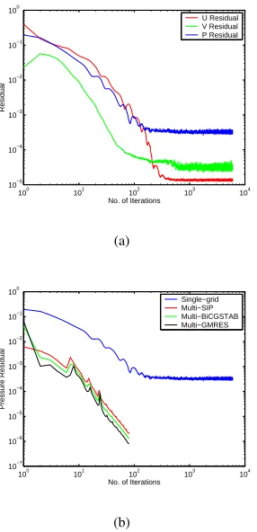
Figure 4(a) displays the convergence history for capillary flow in a single grid with the finest grid spacing. In the current calculation, the energy equation is not considered. The results clearly show that the residuals are reduced effectively in the first 200 outer iterations, and after that, they cannot be further eliminated no matter how many more outer iterations are performed. The results also indicate that the pressure equation has a relatively large residual (Fig. 4(a)).
A comparison was then made between the single-grid and multigrid computations, shown in Fig. 4(b), where the number of iterations means the number of outer iterations on the finest grid (160×20). Only the residual from the pressure equation is
shown as it had the largest value for the single-grid (Fig. 4(a)), but similar differences were found for the other residuals (data not shown). In single-grid computation, the pressure residual can only be reduced to the order of10−3while in the case of
the three-level multigrid computation, it can be reduced to the order of 10−5 within less than 100 outer iterations. Table II
lists the number of outer iterations, CPU-time, and speed-up ratio for the capillary flow with various mesh size and different linear system solvers. In Table II, the recorded CPU-time for multigrid is the total computing time for all levels of grids that are involved. For all three solvers studied (SIP, BiCGSTAB, and GMRES), a great amount of savings in CPU time has been observed by using multigrid. For example, the CPU time needed for a160×20grid using the SIP method was 176.45
seconds for the single-grid and 5.39 for the multigrid. This difference in time was due to the significant difference in the number of outer iterations required which was 6000 for the single-grid and only 54 for the multigrid. This can result in a speed-up ratio for the capillary flow of over 30 for the finest grid. Three iterative solvers, SIP [19], BiCGSTAB [20] and GMRES [17] are used to solve the inner linear system and their performance are compared. In this particular case with a five diagonal coefficient matrix, BiCGSTAB and GMRES solvers do not have obvious advantages over SIP in reducing the number of outer iterations of Navier-Stokes equations in the multigrid computation.
IV. DISCUSSION ANDCONCLUSION
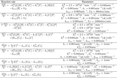
[image:4.612.52.297.62.256.2]TABLE I
THE RATE OF CONCENTRATION CHANGE DUE TO PROTEIN INTERACTIONS(THE INITIAL CONCENTRATION OF SURFACE VARIABLES ARE
R0= 1.6×10⁴receptors/cellANDP0= 3.36×10⁵sites/cell).
Reaction rate Parameters
d[R] dt =−k
R
f[L][R] +kRr[C] +kTr[T]−kc[R][G] kRf = 2.5×10⁸M−1min−1,krR= 0.048min−1
−kint[R] +VR krT = 0.001min−1, kc= 0.001min−1(#/cell)−1
kint= 0.005min−1,VR= 80sites/min d[P]
dt =−k P
f[L][P] +k P r[G] +k
T
r[T]−kc[C][P] kfP = 0.9×10⁸M−1min−1,k P
r = 0.068min−1
−kint[P] +VP krT = 0.001min−1, kc= 0.001min−1(#/cell)−1
kint= 0.005min−1,VP = 1680sites/min
Vddt[L] =−kRf[L][R] +k R
r[C] +kTr[T]−kPf[L][P] k R
f = 2.5×10⁸M−1min−1
−kRr[G] kfP = 0.9×10⁸M−1min−1
kR
r = 0.048min−1,krT = 0.001min−1 d[C]
dt =k R
f[L][R]−k R
r[C]−kc[C][P]−kc[C]2 kfR= 2.5×10⁸M−1min−1
+2kuc[C2]−kint[C] krR= 0.048min−1,kc= 0.001min−1(#/cell)−1
kuc= 1min−1,kint= 0.005min−1
d[C2] dt =
kc
2[C] 2
−kuc[C2]−kintD [C2]
kc= 0.001min−1(#/cell)−1,kuc= 1min−1
kD
int= 0.078min−1 d[G]
dt =−k R
f[L][R] +kRr[C] +kTr[T]−kc[R][G] kfR= 2.5×10⁸M−1min−1
−kint[R] kRr = 0.048min−1,krT = 0.001min−1
kc= 0.001min−1(#/cell)−1,kint= 0.005min−1
d[G2] dt =
kc
2[G] 2
−kuc[G2]−kint[G2] kc= 0.001min
−1(#/cell)−1,k
uc= 1min−1
kD
int= 0.078min−1 d[T]
dt =kc[R][G] +kc[C][P]−k T
r[T]−kc[T]2 kc= 0.001min−1(#/cell)−1,krT = 0.001min−1
+2kuc[T2]−kint[T] kuc= 1min−1,kint= 0.005min−1
d[T2] dt =
kc
2[T] 2
−kuc[T2]−kintD [T2] kc= 0.001min
−1(#/cell)−1,k
uc= 1min−1
kD
int= 0.078min−1
TABLE II
PERFORMANCE COMPARISON OF MULTIGRID METHOD WITH DIFFERENT LINEAR SYSTEM SOLVERS.
Solver Mesh Single-grid MultigridNo. Outer Iterations Single-grid MultigridCPU-Time (s) Speed-up Ratio
SIP 8040××105 234898 23428 0.416.87 0.640.41 10.71.0
160×20 6000 54 176.45 5.39 32.7
BiCGSTAB 8040××105 114432 11426 0.355.24 0.560.35 9.361.0
160×20 6000 50 174.66 5.43 32.16
GMRES 8040××105 101389 10123 0.225.43 0.550.22 9.871.0
160×20 6000 52 186.75 5.82 32.08
movement of FGF-2 is not considered, and reaction-diffusion models [3], [9], which are relatively more complex and the movement of FGF-2 molecules from fluid to cell surface is modeled by diffusion. Filion and Popel [9] proposed a one-dimensional diffusion-reaction model, in which FGF-2,FGF-2 dimers, soluble heparin-like glycosaminoglycans (HLGAGs), FGF-2-HLGAG compounds, and FGF-2-dimer-HLGAG com-pounds are located in the fluid layer. Those molecules move from fluid to cell surface by diffusion. The diffusion model is valid only if the fluid is quiescent, which is not consistent with the actual biological environment of moving bio-fluids. Our model is unique, in which a coupled convection-diffusion-reaction model is applied, and the motion of bio-fluids is fully considered.
We model the process of growth-factor binding and disso-ciation under flow as fluid flow in capillary by
incompress-ible Navier-Stokes equation, protein transport by convection-diffusion, and local bioreaction on capillary surface. The flow is assumed to be laminar, and both the fluid density and viscosity are taken as constants. This is due to the fact that the fluid in the bioreactor fibers is mainly water with some additives (FiberCell Systems, Inc., Frederick, MD, USA). The impact of fluid flow on heparin regulation of FGF binding is through the transport equations in the coupled nonlinear convection-diffusion-reaction model, where the flow velocity affects the distribution of FGF in the solution, and that of FGFR, HSPG, and their compounds on capillary surface.
100 101 102 103 104
10−5
10−4
10−3
10−2
10−1
100
No. of Iterations
Residual
U Residual V Residual P Residual
(a)
100 101 102 103 104
10−7
10−6
10−5
10−4
10−3
10−2
10−1
100
No. of Iterations
Pressure Residual
Single−grid Multi−SIP Multi−BiCGSTAB Multi−GMRES
[image:6.612.110.253.62.358.2](b)
Fig. 4. Comparison of convergence history between single-grid and multigrid computations. (a) Residuals of pressure and velocities in single-grid computa-tion. (b) Comparison of pressure residuals between single-grid and multigrid computation with different linear system solvers.
the linear equations need not be solved very accurately at each outer iteration. Usually a few iterations of a linear system solver is enough. More accurate solution will not reduce the number of outer iterations but may increase the computing time [21].
Three iterative methods - Stone’s SIP, BiCGSTAB, and GMRES - were used to solve the linear systems and their performance is compared. For the simple model system ex-amined, the multigrid methods offered significant speed-up improvement over the single-grid method for all three solvers with all iterative methods yielding similar results.
In conclusion, this paper presents a multigrid computation strategy for the numerical solution of ligand transport and cellular binding within a capillary (i.e., cylindrical geome-try). The capillary flow is predicted using the incompressible Navier-Stokes equations by the finite volume method with collocated mesh arrangement with the assumption that the capillary is a circular pipe. To reduce the computation cost, a multigrid V-cycle technique is applied for the nonlinear Navier-Stokes equations, which includes restriction and pro-longation to restrict fine grid solution to coarse grid, and to interpolate coarse grid solution to fine grid. The multigrid method is extended to solve the mass transport equation. Computational results indicate that the multigrid method can reduce CPU time substantially.
REFERENCES
[1] Brown, P., Byrne, G. and Hindmarsh, A. (1989) “VODE: A variable coefficient ODE solver”, SIAM J. Sci. Stat. Comput., vol. 10, pp.1038-1051.
[2] Chang, K. and Hammer, D. (1999) “The forward rate of binding of surface-tethered reactants: effect of relative motion between two surfaces”, Biophysical J., vol. 76, pp.1280-1292.
[3] Did, C.J., Cooney, C.L. and Nugent, M,A. (1999) “Heparan sulfate mediates bFGF transport through basement membrane by diffusion with rapid reversible binding”, The J. of Biol. Chem., vol. 274, pp.5236-5244. [4] Elhadj, S., Akers, R.M. and Forsten-Williams, K. (2003) “Chronic pulsatile shear stress alters insulin-like growth factor-I (IGF-I) bonding protein releasein vitro”, Annal of Biomed. Engi., vol. 31, pp.163-170. [5] Ezekowitz, A., Mulliken, J. and Folkman J. (1991) “Interferon alpha
therapy of haemangiomas in newborns and infants”, Br. J. Haematol., vol. 79, pp.67-68.
[6] Fannon, M. and Nugent, M.A. (1996) “Basic fibroblast growth factor binds its receptors, is internalized, and stimulates DNA synthesis in Balb/c3T3 cells in the absence of heparan sulfate”, J. Biol. Chem., vol. 271, pp.17949-17956.
[7] Fannon, M., Forsten, K.E. and Nugent, M.A. (2000) “Potentiation and inhibition of bFGF binding by heparin: a model for regulation of cellular response”, Biochemistry, vol. 39, pp.1434-1444.
[8] Ferziger, J.H., Peric´, M. (1999) Computational Methods for Fluid Dynamics, Springer, Berlin
[9] Filion, R.J. and Popel, A.S. (2004) “A reaction-diffusion model of basic fibroblast growth factor interactions with cell surface receptors”, Annal of Biomed. Eng.vol.32, pp.645-663.
[10] Folkman, J. (1995) “Angiogenesis in cancer, vascular, rheumatoid and other disease”, Nat. Med., vol. 1, pp.27-31.
[11] Forsten-Williams, K., Chua, C. and Nugent, M. (2005) “The kinetics of FGF-2 binding to heparan sulfate proteoglycans and MAP kinase signaling”, J. of Theor. Biology, vol. 233, pp.483-499.
[12] Gabhann, F.M., Yang, M.T. and Popel, A.S. (2005) “Monte Carlo sim-ulations of VEGF binding to cell surface receptors in vitro”, Biochimica et Biophysica Acta, vol. 1746, pp.95-107.
[13] Glaser, W. (1993) “Antigen-antibody binding and mass transport by convection and diffusion to a surface: a two-dimensional computer model of binding and dissociation kinetics”, Analy. Biochemistry, vol. 213, pp.152-161.
[14] Itoh, N. (2007) “The Fgf families in humans, mice, and zebrafish: their evolutional processes and roles in development, metabolism, and disease”, Biol. Pharm. Bull., vol. 30, pp.1819-1825.
[15] Myszka, D., He X, et al (1998) “Extending the range of rate constants available from BIACORE: interpreting mass transport-influenced binding data”, Biophysical J., vol. 75, pp. 583-594.
[16] Schreck, E. and Peri´c, M. (1993) “Computation of fluid flow with a parallel multigrid solver”, Int. J .for Numer. Meth. in Fluids, vol. 16, pp.303-327.
[17] Saad, Y. and Schultz, M. (1986) “GMRES: A generalized minimal residual algorithm for solving nonsymmetric linear systems”, SIAM J. Sci. Stat. Comput., vol. 7, pp.856-869.
[18] Shen, W., Zhang, C., Fannon, M., et al (2008) “A Computational Model of FGF-2 Binding and HSPG Regulation Under Flow”, IEEE Tran. on Biom. Engi., in press.
[19] Stone, H. (1968) “Iterative solution of implicit approximations of multidimensional partial differential equations”, SIAM J. of Numer. Analysis, vol. 5, pp.530-558.
[20] Van der Vorst, A. (1992) “Bi-CGSTAB: a fast and smoothly converging variant of Bi-CG for the solution of nonsymmetric linear systems”,SIAM J. Sci. Stat. Comput., vol. 13, pp.631-644.