3313
Benchmarking Approximate Inference Methods
for Neural Structured Prediction
Lifu Tu Kevin Gimpel
Toyota Technological Institute at Chicago, Chicago, IL, 60637, USA {lifu,kgimpel}@ttic.edu
Abstract
Exact structured inference with neural net-work scoring functions is computationally challenging but several methods have been proposed for approximating inference. One approach is to perform gradient descent with respect to the output structure di-rectly (Belanger and McCallum, 2016). An-other approach, proposed recently, is to train a neural network (an “inference network”) to perform inference (Tu and Gimpel,2018). In this paper, we compare these two families of inference methods on three sequence label-ing datasets. We choose sequence labeling because it permits us to use exact inference as a benchmark in terms of speed, accuracy, and search error. Across datasets, we demon-strate that inference networks achieve a better speed/accuracy/search error trade-off than gra-dient descent, while also being faster than ex-act inference at similar accuracy levels. We find further benefit by combining inference networks and gradient descent, using the for-mer to provide a warm start for the latter.1
1 Introduction
Structured prediction models commonly involve complex inference problems for which finding
ex-act solutions is intrex-actable (Cooper,1990). There
are generally two ways to address this difficulty. One is to restrict the model family to those for which inference is feasible. For example, state-of-the-art methods for sequence labeling use struc-tured energies that decompose into label-pair po-tentials and then use rich neural network
archi-tectures to define the potentials (Collobert et al.,
2011; Lample et al., 2016; Ma and Hovy, 2016,
inter alia). Exact dynamic programming algo-rithms like the Viterbi algorithm can be used for inference.
1Code is available at github.com/lifu-tu/
BenchmarkingApproximateInference
The second approach is to retain
computationally-intractable scoring functions
but then use approximate methods for inference. For example, some researchers relax the struc-tured output space from a discrete space to a continuous one and then use gradient descent to maximize the score function with respect to the
output (Belanger and McCallum, 2016). Another
approach is to train a neural network (an “infer-ence network”) to output a structure in the relaxed space that has high score under the structured
scoring function (Tu and Gimpel, 2018). This
idea was proposed as an alternative to gradient descent in the context of structured prediction
energy networks (Belanger and McCallum,2016).
In this paper, we empirically compare exact in-ference, gradient descent, and inference networks for three sequence labeling tasks. We train condi-tional random fields (CRFs) for sequence labeling with neural networks used to define the potentials. We choose a scoring function that permits exact inference via Viterbi so that we can benchmark the approximate methods in terms of search error in addition to speed and accuracy. We consider three families of neural network architectures to serve as inference networks: convolutional neural net-works (CNNs), recurrent neural netnet-works (RNNs), and sequence-to-sequence models with attention
(seq2seq; Sutskever et al., 2014; Bahdanau et al.,
2015). We also use multi-task learning while
train-ing inference networks, combintrain-ing the structured scoring function with a local cross entropy loss.
with Viterbi taking much longer. In this regime, it is difficult for gradient descent to find a good solution, even with many iterations.
In comparing inference network architectures, (1) CNNs are the best choice for tasks with pri-marily local structure, like part-of-speech tagging; (2) RNNs can handle longer-distance dependen-cies while still offering high decoding speeds; and (3) seq2seq networks consistently work better than RNNs, but are also the most computationally ex-pensive.
We also compare search error between gradient descent and inference networks and measure cor-relations with input likelihood. We find that infer-ence networks achieve lower search error on in-stances with higher likelihood (under a pretrained language model), while for gradient descent the correlation between search error and likelihood is closer to zero. This shows the impact of the use of dataset-based learning of inference networks, i.e., they are more effective at amortizing inference for more common inputs.
Finally, we experiment with two refinements of inference networks. The first fine-tunes the infer-ence network parameters for a single test exam-ple to minimize the energy of its output. The sec-ond uses an inference network to provide a warm start for gradient descent. Both lead to reductions in search error and higher accuracies for certain tasks, with the warm start method leading to a bet-ter speed/accuracy trade-off.
2 Sequence Models
For sequence labeling tasks, given an input
se-quence x = hx1, x2, ..., x|x|i, we wish to output
a sequencey = hy1,y2, ...,y|x|i ∈ Y(x). Here
Y(x)is the structured output space forx. Each
la-belytis represented as anL-dimensional one-hot
vector whereLis the number of labels.
Conditional random fields (CRFs;
Lafferty et al., 2001) form one popular class of methods for structured prediction, especially for sequence labeling. We define our structured energy function to be similar to those often used in CRFs for sequence labeling:
EΘ(x,y) =
− X
t L
X
i=1 yt,i
u⊤i f(x, t)+X
t
y⊤t−1Wyt
!
where yt,i is the ith entry of the vector yt. In
the standard discrete-label setting, each yt is a
one-hot vector, but this energy is generalized to be able to use both discrete labels and continu-ous relaxations of the label space, which we will
introduce below. Also, we use f(x, t) ∈ Rd
to denote the “input feature vector” for position
t, ui ∈ Rd is a label-specific parameter vector
used for modeling the local scoring function, and
W ∈ RL×L is a parameter matrix learned to
model label transitions. For the feature vectors we use a bidirectional long short-term memory
(BLSTM;Hochreiter and Schmidhuber,1997), so
this forms a BLSTM-CRF (Lample et al., 2016;
Ma and Hovy,2016).
For training, we use the standard conditional log-likelihood objective for CRFs, using the for-ward and backfor-ward dynamic programming
algo-rithms to compute gradients. For a given inputx
at test time, prediction is done by choosing the out-put with the lowest energy:
argmin y∈Y(x)
EΘ(x,y)
The Viterbi algorithm can be used to solve this problem exactly for the energy defined above.
2.1 Modeling Improvements: BLSTM-CRF+
For our experimental comparison, we consider two CRF variants. The first is the basic model described above, which we refer to as BLSTM-CRF. Below we describe three additional tech-niques that we add to the basic model. We will refer to the CRF with these three techniques as BLSTM-CRF+. Using these two models permits us to assess the impact of model complexity and performance level on the inference method com-parison.
Word Embedding Fine-Tuning. We used pre-trained, fixed word embeddings when using the BLSTM-CRF model, but for the more complex BLSTM-CRF+ model, we fine-tune the pretrained word embeddings during training.
Character-Based Embeddings. Character-based word embeddings provide consistent
im-provements in sequence labeling (Lample et al.,
2016; Ma and Hovy, 2016). In addition to pretrained word embeddings, we produce a character-based embedding for each word using a character convolutional network like that of
sequence in the word and the resulting embedding is concatenated with the word embedding before being passed to the BLSTM.
Dropout. We also add dropout during
train-ing (Hinton et al., 2012). Dropout is applied
be-fore the character embeddings are fed into the CNNs, at the final word embedding layer before the input to the BLSTM, and after the BLSTM. The dropout rate is 0.5 for all experiments.
3 Gradient Descent for Inference
To use gradient descent (GD) for structured infer-ence, researchers typically relax the output space from a discrete, combinatorial space to a continu-ous one and then use gradient descent to solve the following optimization problem:
argmin y∈YR(x)
EΘ(x,y)
whereYRis the relaxed continuous output space.
For sequence labeling,YR(x)consists of
length-|x|sequences of probability distributions over
out-put labels. To obtain a discrete labeling for eval-uation, the most probable label at each position is returned.
There are multiple settings in which gradi-ent descgradi-ent has been used for structured
in-ference, e.g., image generation (Johnson et al.,
2016), structured prediction energy networks
(Belanger and McCallum, 2016), and machine
translation (Hoang et al.,2017). Gradient descent
has the advantage of simplicity. Standard autodif-ferentiation toolkits can be used to compute gradi-ents of the energy with respect to the output once the output space has been relaxed. However, one challenge is maintaining constraints on the vari-ables being optimized. Therefore, we actually per-form gradient descent in an even more relaxed
out-put spaceYR′(x)which consists of length-|x|
se-quences of vectors, where each vector yt ∈ RL.
When computing the energy, we use a softmax
transformation on eachyt, solving the following
optimization problem with gradient descent:
argmin y∈YR′(x)
EΘ(x,softmax(y)) (1)
where the softmax operation above is applied
in-dependently to each vectorytin the output
struc-turey.
4 Inference Networks
Tu and Gimpel (2018) define an inference
net-work(“infnet”)AΨ :X → YR and train it with
the goal that
AΨ(x)≈argmin
y∈YR(x)
EΘ(x,y)
whereYR is the relaxed continuous output space
as defined in Section 3. For sequence labeling,
for example, an inference networkAΨtakes a
se-quencexas input and outputs a distribution over
labels for each position inx. Below we will
con-sider three families of neural network architectures
forAΨ.
For training the inference network parameters
Ψ, Tu and Gimpel (2018) explored stabilization and regularization terms and found that a local cross entropy loss consistently worked well for se-quence labeling. We use this local cross entropy loss in this paper, so we perform learning by solv-ing the followsolv-ing:
argmin Ψ
X
hx,yi
EΘ(x,AΨ(x))+λℓtoken(y,AΨ(x))
where the sum is overhx,yipairs in the training
set. The token-level loss is defined:
ℓtoken(y,A(x)) =
|y| X
t=1
CE(yt,A(x)t) (2)
whereytis theL-dimensional one-hot label
vec-tor at positiontiny, A(x)t is the inference
net-work’s output distribution at position t, and CE
stands for cross entropy. We will give more details
on howℓtokenis defined for different inference
net-work families below. It is also the loss used in our non-structured baseline models.
4.1 Inference Network Architectures
We now describe options for inference network ar-chitectures for sequence labeling. For each, we optionally include the modeling improvements
de-scribed in Section2.1. When doing so, we append
“+” to the setting’s name to indicate this (e.g., infnet+).
4.1.1 Convolutional Neural Networks
CNNs are frequently used in NLP to ex-tract features based on symbol subsequences,
whether words or characters (Collobert et al.,
Kim et al., 2016;Zhang et al., 2015). CNNs use filters that are applied to symbol sequences and are typically followed by some sort of pooling opera-tion. We apply filters over a fixed-size window centered on the word being labeled and do not use
pooling. The feature mapsfn(x, t)for(2n+ 1)
-gram filters are defined:
fn(x, t) =g(Wn[vxt−n;...;vxt+n] +bn)
where g is a nonlinearity, vxt is the embedding
of wordxt, andWnandbnare filter parameters.
We consider two CNN configurations: one uses
n = 0andn = 1and the other usesn = 0and
n = 2. For each, we concatenate the two feature
maps and use them as input to the softmax layer
over outputs. In each case, we use H filters for
each feature map.
4.1.2 Recurrent Neural Networks
For sequence labeling, it is common to use a BLSTM that runs over the input sequence and pro-duces a softmax distribution over labels at each position in the sequence. We use this “BLSTM tagger” as our RNN inference network
architec-ture. The parameterHrefers to the size of the
hid-den vectors in the forward and backward LSTMs, so the full dimensionality passed to the softmax
layer is2H.
4.1.3 Sequence-to-Sequence Models
Sequence-to-sequence (seq2seq; Sutskever et al.
2014) models have been successfully used for
many sequential modeling tasks. It is
com-mon to augment models with an attention mech-anism that focuses on particular positions of the input sequence while generating the
out-put sequence (Bahdanau et al., 2015). Since
se-quence labeling tasks have equal input and out-put sequence lengths and a strong connection between corresponding entries in the sequences,
Goyal et al.(2018) used fixed attention that
deter-ministically attends to theith input when decoding
theith output, and hence does not learn any
atten-tion parameters. It is shown as follows:
P(yt|y<t,x) = softmax(Ws[ht,st])
where st is the hidden vector at position t from
a BLSTM run over x, ht is the decoder hidden
vector at position t, and Ws is a parameter
ma-trix. The concatenation of the two hidden vectors is used to produce the distribution over labels.
When using this inference network, we redefine the local loss to the standard training criterion for seq2seq models, namely the sum of the log losses for each output conditioned on the previous out-puts in the sequence. We always use the previ-ous predicted label as input (as used in “scheduled
sampling,”Bengio et al.,2015) during training
be-cause it works better for our tasks. In our experi-ments, the forward and backward encoder LSTMs
use hidden dimensionH, as does the LSTM
de-coder. Thus the model becomes similar to the BLSTM tagger except with conditioning on pre-vious labeling decisions in a left-to-right manner.
We also experimented with the use of beam search for both the seq2seq baseline and infer-ence networks and did not find much differ-ence in the results. Also, as alternatives to the deterministic position-based attention described above, we experimented with learned local
atten-tion (Luong et al.,2015) and global attention, but
they did not work better on our tasks.
4.2 Methods to Improve Inference Networks
To further improve the performance of an
infer-ence network for a particular test instancex, we
propose two novel approaches that leverage the strengths of inference networks to provide effec-tive starting points and then use instance-level fine-tuning in two different ways.
4.2.1 Instance-Tailored Inference Networks
For each test examplex, we initialize an
instance-specific inference network AΨ(x) using the
trained inference network parameters, then run gradient descent on the following loss:
argmin Ψ
EΘ(x,AΨ(x)) (3)
This procedure fine-tunes the inference network parameters for a single test example to minimize
the energy of its output. For each test
exam-ple, the process is repeated, with a new instance-specific inference network being initialized from the trained inference network parameters.
4.2.2 Warm-Starting Gradient Descent with Inference Networks
Given a test examplex, we initializey∈ YR′(x)
using the inference network and then use gradient
descent by solving Eq.1described in Section3to
updatey. However, the inference network output
more relaxed spaceYR′(x). So we simply use the
logits from the inference network, which are the score vectors before the softmax operations.
5 Experimental Setup
We perform experiments on three tasks: Twit-ter part-of-speech tagging (POS), named entity recognition (NER), and CCG supersense tagging (CCG).
5.1 Datasets
POS. We use the annotated data from
Gimpel et al. (2011) and Owoputi et al. (2013) which contains 25 POS tags. For training, we
combine the 1000-tweet OCT27TRAIN set and
the 327-tweet OCT27DEV set. For validation,
we use the 500-tweet OCT27TEST set and for
testing we use the 547-tweet DAILY547 test
set. We use the 100-dimensional skip-gram
embeddings from Tu et al. (2017) which were
trained on a dataset of 56 million English tweets
using word2vec (Mikolov et al., 2013). The
evaluation metric is tagging accuracy.
NER. We use the CoNLL 2003 English data
(Tjong Kim Sang and De Meulder, 2003). There are four entity types: PER, LOC, ORG, and MISC. There is a strong local dependency between neigh-boring labels because this is a labeled segmenta-tion task. We use the BIOES tagging scheme, so there are 17 labels. We use 100-dimensional
pre-trained GloVe (Pennington et al., 2014)
embed-dings. The task is evaluated with micro-averaged
F1 score using theconllevalscript.
CCG. We use the standard splits from
CCG-bank (Hockenmaier and Steedman, 2002). We
only keep sentences with length less than 50 in the original training data when training the CRF. The training data contains 1,284 unique labels, but because the label distribution has a long tail, we use only the 400 most frequent labels, replacing
the others by a special tag∗. The percentages of
∗ in train/development/test are 0.25/0.23/0.23%.
When the gold standard tag is∗, the prediction is
always evaluated as incorrect. We use the same GloVe embeddings as in NER. Because of the compositional nature of supertags, this task has more non-local dependencies. The task is evalu-ated with per-token accuracy.
5.2 Training and Tuning
For the optimization problems mentioned below, we use stochastic gradient descent with momen-tum as the optimizer. Full details of hyperparame-ter tuning are in the appendix.
Local Baselines. We consider local (non-structured) baselines that use the same architec-tures as the inference networks but train using
only the local lossℓtoken.
Structured Baselines. We train the BLSTM-CRF and BLSTM-BLSTM-CRF+ models with the standard conditional log-likelihood objective. We tune hy-perparameters on the development sets.
Gradient Descent for Inference. We use gra-dient descent for structured inference by solving
Eq. 1. We randomly initialize y ∈ YR′(x) and,
for N iterations, we compute the gradient of the
energy with respect toy, then updateyusing
gra-dient descent with momentum, which we found to generally work better than constant step size. We
tuneN and the learning rate via instance-specific
oracle tuning, i.e., we choose them separately for each input to maximize performance (accuracy or F1 score) on that input. Even with this oracle tun-ing, we find that gradient descent struggles to com-pete with the other methods.
Inference Networks. To train the inference net-works, we first train the CRF or BLSTM-CRF+ model with the standard conditional
log-likelihood objective. The hidden sizesHare tuned
in that step. We then fix the energy function and
train the inference network AΨ using the
com-bined loss from Section4.
For instance-tailored inference networks and when using inference networks as a warm start for
gradient descent, we tune the number of epochsN
and the learning rate on the development set, and report the performance on the test set, using the
same values ofN and the learning rate for all test
examples.
6 BLSTM-CRF Results
This first section of results uses the simpler
BLSTM-CRF modeling configuration. In
Sec-tion 7below we present results with the stronger
Twitter POS Tagging NER CCG Supertagging CNN BLSTM seq2seq CNN BLSTM seq2seq CNN BLSTM seq2seq
local baseline 89.6 88.0 88.9 79.9 85.0 85.3 90.6 92.2 92.7
infnet 89.9 89.5 89.7 82.2 85.4 86.1 91.3 92.8 92.9
gradient descent 89.1 84.4 89.0
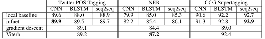
[image:6.595.88.511.63.126.2]Viterbi 89.2 87.2 92.4
Table 1: Test results for all tasks. Inference networks, gradient descent, and Viterbi are all optimizing the BLSTM-CRF energy. Best result per task is in bold.
Table 1 shows test results for all tasks and
ar-chitectures. The inference networks use the same architectures as the corresponding local baselines, but their parameters are trained with both the local loss and the BLSTM-CRF energy, leading to con-sistent improvements. CNN inference networks work well for POS, but struggle on NER and CCG compared to other architectures. BLSTMs work well, but are outperformed slightly by seq2seq models across all three tasks. Using the Viterbi algorithm for exact inference yields the best per-formance for NER but is not best for the other two tasks.
It may be surprising that an inference network trained to mimic Viterbi would outperform Viterbi in terms of accuracy, which we find for the CNN for POS tagging and the seq2seq inference net-work for CCG. We suspect this occurs for two
reasons. One is due to the addition of the
lo-cal loss in the inference network objective; the inference networks may be benefiting from this
multi-task training.Edunov et al.(2018) similarly
found benefit from a combination of token-level and sequence-level losses. The other potential rea-son is beneficial inductive bias with the inference network architecture. For POS tagging, the CNN architecture is clearly well-suited to this task given the strong performance of the local CNN baseline. Nonetheless, the CNN inference network is able to improve upon both the CNN baseline and Viterbi.
Hidden Sizes. For the test results in Table1, we
did limited tuning ofHfor the inference networks
based on the development sets. Figure 1 shows
the impact ofH on performance. AcrossH
val-ues, the inference networks outperform the base-lines. For NER and CCG, seq2seq outperforms the BLSTM which in turn outperforms the CNN.
Tasks and Window Sizes. Table 2 shows that CNNs with smaller windows are better for POS, while larger windows are better for NER and CCG. This suggests that POS has more local de-pendencies among labels than NER and CCG.
Hidden size
0 100 200 300
F1
80 82 84 86 88 90 92
(a) NER
Hidden size
200 400 600 800 1000
Accuracy(%)
89 89.5 90 90.5 91 91.5 92 92.5 93 93.5
Baseline(CNNs) Baseline(BLSTM) Baseline(seq2seq) InfNet(CNNs) InfNet(BLSTM) InfNet(seq2seq)
[image:6.595.313.518.184.322.2](b) CCG Supertagging
Figure 1: Development results for inference networks with different architectures and hidden sizes (H).
{1,3}-gram {1,5}-gram
POS local baseline 89.2 88.7
infnet 89.6 89.0
NER local baseline 84.6 85.4
infnet 86.7 86.8
CCG local baseline 89.5 90.4
infnet 90.3 91.4
Table 2: Development results for CNNs with two filter sets (H = 100).
6.1 Speed Comparison
Asymptotically, Viterbi takesO(nL2)time, where
n is the sequence length. The BLSTM and our
deterministic-attention seq2seq models have time
complexity O(nL). CNNs also have
complex-ityO(nL)but are more easily parallelizable.
Ta-ble 3 shows test-time inference speeds for
infer-ence networks, gradient descent, and Viterbi for the BLSTM-CRF model. We use GPUs and a minibatch size of 10 for all methods. CNNs are 1-2 orders of magnitude faster than the others. BLSTMs work almost as well as seq2seq models and are 2-4 times faster in our experiments. Viterbi
is actually faster than seq2seq when L is small,
but for CCG, which hasL = 400, it is 4-5 times
[image:6.595.314.518.375.448.2]CNN BLSTM seq2seq Viterbi GD
POS 12500 1250 357 500 20
NER 10000 1000 294 360 23
CCG 6666 1923 1000 232 16
Table 3: Speed comparison of inference networks across tasks and architectures (examples/sec).
6.2 Search Error
We can view inference networks as approximate search algorithms and assess characteristics that affect search error. To do so, we train two LSTM language models (one on word sequences and one on gold label sequences) on the Twitter POS data. We also compute the difference in the BLSTM-CRF energies between the inference network
out-putyinf and the Viterbi outputyvit as the search
error: EΘ(x,yinf)−EΘ(x,yvit). We compute
the same search error for gradient descent. For the BLSTM inference network, Spearman’s
ρ between the word sequence perplexity and
search error is 0.282; for the label sequence per-plexity, it is 0.195. For gradient descent
infer-ence, Spearman’s ρ between the word sequence
perplexity and search error is 0.122; for the la-bel sequence perplexity, it is 0.064. These positive correlations mean that for frequent sequences, in-ference networks and gradient descent exhibit less search error. We also note that the correlations are higher for the inference network than for gradi-ent descgradi-ent, showing the impact of amortization during learning of the inference network parame-ters. That is, since we are learning to do inference from a dataset, we would expect search error to be smaller for more frequent sequences, and we do indeed see this correlation.
7 BLSTM-CRF+ Results
We now compare inference methods when using the improved modeling techniques described in
Section 2.1 (i.e., the setting we called
BLSTM-CRF+). We use these improved techniques for all models, including the CRF, the local base-lines, gradient descent, and the inference net-works. When training inference networks, both the inference network architectures and the
struc-tured energies use the techniques from Section2.1.
So, when referring to inference networks in this section, we use the name infnet+.
The results are shown in Table4. With a more
powerful local architecture, structured prediction is less helpful overall, but inference networks still
POS NER CCG
local baseline 91.3 90.5 94.1
infnet+ 91.3 90.8 94.2
gradient descent 90.8 89.8 90.4
[image:7.595.85.276.62.104.2]Viterbi 90.9 91.6 94.3
Table 4: Test results with BLSTM-CRF+. For local baseline and inference network architectures, we use CNN for POS, seq2seq for NER, and BLSTM for CCG.
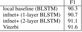
F1 local baseline (BLSTM) 90.3 infnet+ (1-layer BLSTM) 90.7 infnet+ (2-layer BLSTM) 91.1
Viterbi 91.6
Table 5: NER test results (for BLSTM-CRF+) with more layers in the BLSTM inference network.
improve over the local baselines on 2 of 3 tasks.
POS. As in the BLSTM-CRF setting, the local
CNN baseline and the CNN inference network
outperform Viterbi. This is likely because the
CRFs use BLSTMs as feature networks, but our results show that CNN baselines are consistently better than BLSTM baselines on this task. As in the BLSTM-CRF setting, gradient descent works quite well on this task, comparable to Viterbi, though it is still much slower.
NER. We see slightly higher BLSTM-CRF+
results than several previous state-of-the-art
results (cf. 90.94; Lample et al., 2016 and
91.37; Ma and Hovy, 2016). The stronger
BLSTM-CRF+ configuration also helps the infer-ence networks, improving performance from 90.5 to 90.8 for the seq2seq architecture over the local baseline. Though gradient descent reached high accuracies for POS tagging, it does not perform well on NER, possibly due to the greater amount of non-local information in the task.
While we see strong performance with infnet+, it still lags behind Viterbi in F1. We consider addi-tional experiments in which we increase the num-ber of layers in the inference networks. We use a 2-layer BLSTM as the inference network and also use weight annealing of the local loss
hyper-parameter λ, setting it to λ = e−0.01t wheretis
the epoch number. Without this annealing, the 2-layer inference network was difficult to train. The weight annealing was helpful for encourag-ing the inference network to focus more on the non-local information in the energy function rather
than the token-level loss. As shown in Table 5,
[image:7.595.337.499.63.114.2] [image:7.595.352.483.172.224.2]Twitter POS Tagging NER CCG Supertagging
N Acc.(↑) Energy(↓) F1(↑) Energy(↓) Acc.(↑) Energy(↓)
gold standard 100 -159.65 100 -230.63 100 -480.07
BLSTM-CRF+/Viterbi 90.9 -163.20 91.6 -231.53 94.3 -483.09
10 89.2 -161.69 81.9 -227.92 65.1 -412.81
20 90.8 -163.06 89.1 -231.17 74.6 -414.81
30 90.8 -163.02 89.6 -231.30 83.0 -447.64
gradient descent 40 90.7 -163.03 89.8 -231.34 88.6 -471.52
50 90.8 -163.04 89.8 -231.35 90.0 -476.56
100 - - - - 90.1 -476.98
500 - - - - 90.1 -476.99
1000 - - - - 90.1 -476.99
infnet+ 91.3 -162.07 90.8 -231.19 94.2 -481.32
discretized output from infnet+ 91.3 -160.87 90.8 -231.34 94.2 -481.95
3 91.0 -162.59 91.3 -231.32 94.3 -481.91
instance-tailored infnet+ 5 90.9 -162.81 91.2 -231.37 94.3 -482.23
10 91.3 -162.85 91.5 -231.39 94.3 -482.56
infnet+ as warm start for 3 91.4 -163.06 91.4 -231.42 94.4 -482.62
gradient descent 5 91.2 -163.12 91.4 -231.45 94.4 -482.64
[image:8.595.91.508.60.276.2]10 91.2 -163.15 91.5 -231.46 94.4 -482.78
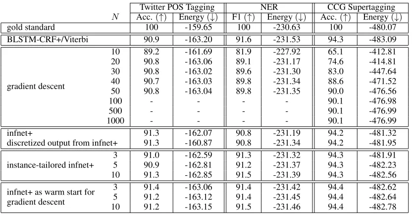
Table 6: Test set results of approximate inference methods for three tasks, showing performance metrics (accuracy and F1) as well as average energy of the output of each method. The inference network architectures in the above experiments are: CNN for POS, seq2seq for NER, and BLSTM for CCG.N is the number of epochs for GD inference or instance-tailored fine-tuning.
CCG. Our BLSTM-CRF+ reaches an accuracy
of 94.3%, which is comparable to several recent
results (93.53,Xu et al., 2016; 94.3, Lewis et al.,
2016; and 94.50, Vaswani et al., 2016). The
lo-cal baseline, the BLSTM inference network, and Viterbi are all extremely close in accuracy. Gradi-ent descGradi-ent struggles here, likely due to the large number of candidate output labels.
7.1 Speed, Accuracy, and Search Error
Table 6 compares inference methods in terms of
both accuracy and energies reached during
infer-ence. For each number N of gradient descent
it-erations in the table, we tune the learning rate per-sentence and report the average accuracy/F1 with that fixed number of iterations. We also report the average energy reached. For inference networks, we report energies both for the output directly and when we discretize the output (i.e., choose the most probable label at each position).
Gradient Descent Across Tasks. The number of gradient descent iterations required for compet-itive performance varies by task. For POS, 20 iter-ations are sufficient to reach accuracy and energy close to Viterbi. For NER, roughly 40 iterations are needed for gradient descent to reach its high-est F1 score, and for its energy to become very close to that of the Viterbi outputs. However, its F1 score is much lower than Viterbi. For CCG, gradient descent requires far more iterations,
pre-sumably due to the larger number of labels in the task. Even with 1000 iterations, the accuracy is 4% lower than Viterbi and the inference works. Unlike POS and NER, the inference net-work reaches much lower energies than gradient descent on CCG, suggesting that the inference net-work may not suffer from the same challenges of searching high-dimensional label spaces as those faced by gradient descent.
Inference Networks Across Tasks. For POS, the inference network does not have lower energy
than gradient descent with≥ 20 iterations, but it
does have higher accuracy. This may be due in part to our use of multi-task learning for inference networks. The discretization of the inference net-work outputs increases the energy on average for this task, whereas it decreases the energy for the other two tasks. For NER, the inference network reaches a similar energy as gradient descent, es-pecially when discretizing the output, but is con-siderably better in F1. The CCG tasks shows the largest difference between gradient descent and the inference network, as the latter is much better in both accuracy and energy.
Instance Tailoring and Warm Starting.
Across tasks, instance tailoring and warm
start-ing lead to lower energies than infnet+. The
Time(s)
0 50 100 150 200 250 300 350
Accuracy(%)
40 60 80 100
Viterbi GD infnet+
Instance-Tailored infnet+ infnet+ warm start for GD 5
10
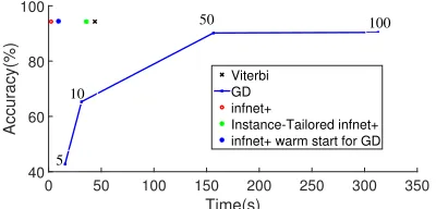
[image:9.595.78.278.68.164.2]100 50
Figure 2: CCG test results for inference methods (GD = gradient descent). The x-axis is the total inference time for the test set. The numbers on the GD curve are the number of gradient descent iterations.
Warm starting gradient descent yields the lowest energies (other than Viterbi), showing promise for the use of gradient descent as a local search method starting from inference network output.
Wall Clock Time Comparison. Figure2shows the speed/accuracy trade-off for the inference methods, using wall clock time for test set infer-ence as the speed metric. On this task, Viterbi is time-consuming because of the larger label set size. The inference network has comparable accu-racy to Viterbi but is much faster. Gradient descent needs much more time to get close to the others but plateaus before actually reaching similar accu-racy. Instance-tailoring and warm starting reside between infnet+ and Viterbi, with warm starting being significantly faster because it does not re-quire updating inference network parameters.
8 Related Work
The most closely related prior work is that of
Tu and Gimpel (2018), who experimented with RNN inference networks for sequence labeling. We compared three architectural families, showed the relationship between optimal architectures and downstream tasks, compared inference networks to gradient descent, and proposed novel variations. We focused in this paper on sequence label-ing, in which CRFs with neural network po-tentials have emerged as a state-of-the-art
ap-proach (Lample et al.,2016;Ma and Hovy,2016;
Strubell et al., 2017; Yang et al., 2018). Our re-sults suggest that inference networks can provide a feasible way to speed up test-time inference over Viterbi without much loss in performance. The benefits of inference networks may be coming in
part from multi-task training;Edunov et al.(2018)
similarly found benefit from combining
token-level and sequence-token-level losses.
We focused on structured prediction in this pa-per, but inference networks are useful in other set-tings as well. For example, it is common to use a particular type of inference network to approx-imate posterior inference in neural approaches to latent-variable probabilistic modeling, such
as variational autoencoders (Kingma and Welling,
2013) and, more closely related to this paper,
vari-ational sequential labelers (Chen et al., 2018). In
such settings,Kim et al.(2018) have found benefit
with instance-specific updating of inference net-work parameters, which is related to our instance-level fine-tuning. There are also connections be-tween structured inference networks and
amor-tized structured inference (Srikumar et al., 2012)
as well as methods for neural knowledge
distilla-tion and model compression (Hinton et al.,2015;
Ba and Caruana,2014;Kim and Rush,2016). Gradient descent is used for inference in sev-eral settings, e.g., structured prediction energy
networks (Belanger and McCallum,2016), image
generation applications (Mordvintsev et al.,2015;
Gatys et al., 2015), finding adversarial examples (Goodfellow et al.,2015), learning paragraph
em-beddings (Le and Mikolov, 2014), and machine
translation (Hoang et al.,2017). Gradient descent
has started to be replaced by inference networks in some of these settings, such as image
transfor-mation (Johnson et al.,2016;Li and Wand,2016).
Our results provide more evidence that gradient descent can be replaced by inference networks or improved through combination with them.
9 Conclusion
We compared several methods for approximate inference in neural structured prediction, find-ing that inference networks achieve a better speed/accuracy/search error trade-off than gradi-ent descgradi-ent. We also proposed instance-level in-ference network fine-tuning and using inin-ference networks to initialize gradient descent, finding fur-ther reductions in search error and improvements in performance metrics for certain tasks.
Acknowledgments
References
Jimmy Ba and Rich Caruana. 2014. Do deep nets really need to be deep? In Z. Ghahramani, M. Welling, C. Cortes, N. D. Lawrence, and K. Q. Weinberger, editors,Advances in Neural Information Processing Systems 27, pages 2654–2662.
Dzmitry Bahdanau, Kyunghyun Cho, and Yoshua Ben-gio. 2015. Neural machine translation by jointly learning to align and translate. In Proceedings of International Conference on Learning Representa-tions (ICLR).
David Belanger and Andrew McCallum. 2016. Struc-tured prediction energy networks. In Proceedings of the 33rd International Conference on Machine Learning - Volume 48, ICML’16, pages 983–992.
Samy Bengio, Oriol Vinyals, Navdeep Jaitly, and Noam Shazeer. 2015. Scheduled sampling for sequence prediction with recurrent neural net-works. In C. Cortes, N. D. Lawrence, D. D. Lee, M. Sugiyama, and R. Garnett, editors,Advances in Neural Information Processing Systems 28, pages 1171–1179.
Mingda Chen, Qingming Tang, Karen Livescu, and Kevin Gimpel. 2018. Variational sequential labelers for semi-supervised learning. InProceedings of the 2018 Conference on Empirical Methods in Natural Language Processing, pages 215–226.
Ronan Collobert, Jason Weston, L´eon Bottou, Michael Karlen, Koray Kavukcuoglu, and Pavel Kuksa. 2011. Natural language processing (almost) from scratch. Journal of Machine Learning Research, 12.
Gregory F. Cooper. 1990. The computational complex-ity of probabilistic inference using Bayesian belief networks (research note). Artif. Intell., 42(2-3).
Sergey Edunov, Myle Ott, Michael Auli, David Grang-ier, and Marc’Aurelio Ranzato. 2018. Classical structured prediction losses for sequence to se-quence learning. In Proceedings of the 2018 Con-ference of the North American Chapter of the Asso-ciation for Computational Linguistics: Human Lan-guage Technologies, Volume 1 (Long Papers), pages 355–364, New Orleans, Louisiana.
Leon A. Gatys, Alexander S. Ecker, and Matthias Bethge. 2015. A neural algorithm of artistic style. CoRR, abs/1508.06576.
Kevin Gimpel, Nathan Schneider, Brendan O’Connor, Dipanjan Das, Daniel Mills, Jacob Eisenstein, Michael Heilman, Dani Yogatama, Jeffrey Flani-gan, and Noah A. Smith. 2011. Part-of-speech tag-ging for Twitter: annotation, features, and experi-ments. In Proceedings of the 49th Annual Meet-ing of the Association for Computational LMeet-inguis- Linguis-tics: Human Language Technologies, pages 42–47, Portland, Oregon, USA.
Ian Goodfellow, Jonathon Shlens, and Christian Szegedy. 2015. Explaining and harnessing adversar-ial examples. InProceedings of International Con-ference on Learning Representations (ICLR).
Kartik Goyal, Graham Neubig, Chris Dyer, and Tay-lor Berg-Kirkpatrick. 2018. A continuous relaxation of beam search for end-to-end training of neural se-quence models. InProceedings of the Thirty-Second AAAI Conference on Artificial Intelligence (AAAI), New Orleans, Louisiana.
Geoffrey Hinton, Oriol Vinyals, and Jeffrey Dean. 2015. Distilling the knowledge in a neural network. InNIPS Deep Learning Workshop.
Geoffrey E. Hinton, Nitish Srivastava, Alex Krizhevsky, Ilya Sutskever, and Ruslan Salakhut-dinov. 2012. Improving neural networks by preventing co-adaptation of feature detectors. CoRR, abs/1207.0580.
Cong Duy Vu Hoang, Gholamreza Haffari, and Trevor Cohn. 2017. Towards decoding as continuous opti-misation in neural machine translation. In Proceed-ings of the 2017 Conference on Empirical Methods in Natural Language Processing, pages 146–156, Copenhagen, Denmark.
Sepp Hochreiter and J¨urgen Schmidhuber. 1997. Long short-term memory.Neural Computation.
Julia Hockenmaier and Mark Steedman. 2002. Acquir-ing compact lexicalized grammars from a cleaner treebank. InProceedings of the Third International Conference on Language Resources and Evaluation, LREC 2002, May 29-31, 2002, Las Palmas, Canary Islands, Spain.
Justin Johnson, Alexandre Alahi, and Li Fei-Fei. 2016. Perceptual losses for real-time style transfer and super-resolution. InProceedings of European Con-ference on Computer Vision (ECCV).
Nal Kalchbrenner, Edward Grefenstette, and Phil Blun-som. 2014. A convolutional neural network for modelling sentences. In Proceedings of the 52nd Annual Meeting of the Association for Computa-tional Linguistics (Volume 1: Long Papers), pages 655–665, Baltimore, Maryland.
Yoon Kim. 2014. Convolutional neural networks for sentence classification. In Proceedings of the 2014 Conference on Empirical Methods in Natural Language Processing (EMNLP), pages 1746–1751, Doha, Qatar.
Yoon Kim, Yacine Jernite, David Sontag, and Alexan-der M. Rush. 2016. Character-aware neural lan-guage models. InProceedings of the Thirtieth AAAI Conference on Artificial Intelligence, AAAI’16, pages 2741–2749. AAAI Press.
2016 Conference on Empirical Methods in Natu-ral Language Processing, pages 1317–1327, Austin, Texas.
Yoon Kim, Sam Wiseman, Andrew Miller, David Son-tag, and Alexander Rush. 2018. Semi-amortized variational autoencoders. InProceedings of the 35th International Conference on Machine Learning, vol-ume 80 of Proceedings of Machine Learning Re-search, pages 2678–2687, Stockholmsmssan, Stock-holm Sweden.
Diederik Kingma and Max Welling. 2013. Auto-encoding variational Bayes. CoRR, abs/1312.6114.
John D. Lafferty, Andrew McCallum, and Fernando C. N. Pereira. 2001. Conditional random fields: Probabilistic models for segmenting and labeling se-quence data. InProceedings of the Eighteenth Inter-national Conference on Machine Learning, ICML ’01, pages 282–289.
Guillaume Lample, Miguel Ballesteros, Sandeep Sub-ramanian, Kazuya Kawakami, and Chris Dyer. 2016. Neural architectures for named entity recognition. InProceedings of the 2016 Conference of the North American Chapter of the Association for Computa-tional Linguistics: Human Language Technologies, pages 260–270, San Diego, California.
Quoc Le and Tomas Mikolov. 2014. Distributed repre-sentations of sentences and documents. In Proceed-ings of the 31st International Conference on Inter-national Conference on Machine Learning - Volume 32, ICML’14.
Mike Lewis, Kenton Lee, and Luke Zettlemoyer. 2016. LSTM CCG parsing. In Proceedings of the 2016 Conference of the North American Chapter of the Association for Computational Linguistics: Human Language Technologies, pages 221–231, San Diego, California.
Chuan Li and Michael Wand. 2016. Precomputed real-time texture synthesis with Markovian gener-ative adversarial networks. In Proceedings of Eu-ropean Conference on Computer Vision (ECCV), pages 702–716.
Thang Luong, Hieu Pham, and Christopher D. Man-ning. 2015. Effective approaches to attention-based neural machine translation. In Proceedings of the 2015 Conference on Empirical Methods in Natu-ral Language Processing, pages 1412–1421, Lisbon, Portugal.
Xuezhe Ma and Eduard Hovy. 2016. End-to-end se-quence labeling via bi-directional lstm-cnns-crf. In Proceedings of the 54th Annual Meeting of the As-sociation for Computational Linguistics (Volume 1: Long Papers), pages 1064–1074, Berlin, Germany.
Tomas Mikolov, Ilya Sutskever, Kai Chen, Greg S Cor-rado, and Jeff Dean. 2013. Distributed representa-tions of words and phrases and their composition-ality. In C. J. C. Burges, L. Bottou, M. Welling,
Z. Ghahramani, and K. Q. Weinberger, editors, Ad-vances in Neural Information Processing Systems 26, pages 3111–3119.
Alexander Mordvintsev, Christopher Olah, and Mike Tyka. 2015. DeepDream-a code example for visual-izing neural networks. Google Research.
Olutobi Owoputi, Brendan O’Connor, Chris Dyer, Kevin Gimpel, Nathan Schneider, and Noah A. Smith. 2013. Improved part-of-speech tagging for online conversational text with word clusters. In Proceedings of the 2013 Conference of the North American Chapter of the Association for Computa-tional Linguistics: Human Language Technologies, pages 380–390, Atlanta, Georgia.
Jeffrey Pennington, Richard Socher, and Christopher Manning. 2014. GloVe: Global vectors for word representation. In Proceedings of the 2014 Con-ference on Empirical Methods in Natural Language Processing (EMNLP), pages 1532–1543, Doha, Qatar.
Vivek Srikumar, Gourab Kundu, and Dan Roth. 2012. On amortizing inference cost for structured predic-tion. In Proceedings of the 2012 Joint Confer-ence on Empirical Methods in Natural Language Processing and Computational Natural Language Learning, pages 1114–1124, Jeju Island, Korea.
Emma Strubell, Patrick Verga, David Belanger, and Andrew McCallum. 2017. Fast and accurate en-tity recognition with iterated dilated convolutions. In Proceedings of the 2017 Conference on Empiri-cal Methods in Natural Language Processing, pages 2670–2680, Copenhagen, Denmark.
Ilya Sutskever, Oriol Vinyals, and Quoc V Le. 2014. Sequence to sequence learning with neural net-works. In Z. Ghahramani, M. Welling, C. Cortes, N. D. Lawrence, and K. Q. Weinberger, editors, Ad-vances in Neural Information Processing Systems 27, pages 3104–3112.
Erik F. Tjong Kim Sang and Fien De Meulder. 2003. Introduction to the CoNLL-2003 shared task: Language-independent named entity recognition. In Proceedings of the Seventh Conference on Natu-ral Language Learning at HLT-NAACL 2003, pages 142–147.
Lifu Tu and Kevin Gimpel. 2018. Learning ap-proximate inference networks for structured predic-tion. InProceedings of International Conference on Learning Representations (ICLR).
Lifu Tu, Kevin Gimpel, and Karen Livescu. 2017. Learning to embed words in context for syntactic tasks. InProceedings of the 2nd Workshop on Rep-resentation Learning for NLP, pages 265–275, Van-couver, Canada.
Linguistics: Human Language Technologies, pages 232–237, San Diego, California.
Wenduan Xu, Michael Auli, and Stephen Clark. 2016. Expected F-measure training for shift-reduce pars-ing with recurrent neural networks. In Proceed-ings of the 2016 Conference of the North Ameri-can Chapter of the Association for Computational Linguistics: Human Language Technologies, pages 210–220, San Diego, California.
Jie Yang, Shuailong Liang, and Yue Zhang. 2018. De-sign challenges and misconceptions in neural se-quence labeling. In Proceedings of the 27th Inter-national Conference on Computational Linguistics, pages 3879–3889, Santa Fe, New Mexico, USA.
Xiang Zhang, Junbo Zhao, and Yann LeCun. 2015. Character-level convolutional networks for text clas-sification. In C. Cortes, N. D. Lawrence, D. D. Lee, M. Sugiyama, and R. Garnett, editors,Advances in Neural Information Processing Systems 28, pages 649–657.
A Appendix
Local Baselines. We consider local (non-structured) baselines that use the same architec-tures as the inference networks but train using
only the local lossℓtoken. We tune the learning rate
({5,1,0.5,0.1,0.05,0.01,0.005,0.001,0.0005}). We train on the training set, use the development sets for tuning and early stopping, and report results on the test sets.
Structured Baselines. We train the BLSTM-CRF and BLSTM-BLSTM-CRF+ models with the stan-dard conditional log-likelihood objective. We tune hyperparameters on the development sets. The
tuned BLSTM hidden sizeH for BLSTM-CRF is
100 for POS/NER and 512 for CCG; for BLSTM-CRF+ the tuned hidden size is 100 for POS, 200 for NER, and 400 for CCG.
Gradient Descent for Inference. For the
num-ber of epochs N, we consider values in the
set {5,10,20,30,40,50,100,500,1000}. For
each N, we tune the learning rate over the
set {1e4,5e3,1e3,500,100,50,10,5,1}). These
learning rates may appear extremely large when we are accustomed to choosing rates for empiri-cal risk minimization, but we generally found that the most effective learning rates for structured in-ference are orders of magnitude larger than those effective for learning. To provide as strong perfor-mance as possible for the gradient descent method,
we tuneN and the learning rate via oracle tuning,
i.e., we choose them separately for each input to
maximize performance (accuracy or F1 score) on that input.
Inference Networks. To train the inference networks, we first train the BLSTM-CRF or BLSTM-CRF+ model with the standard
con-ditional log-likelihood objective. The hidden
sizes H are tuned in that step. We then fix
the energy function and train the inference
network AΨ using the combined loss from
Section 4. We tune the learning rate over the set
{5,1,0.5,0.1,0.05,0.01,0.005,0.001,0.0005}
for the inference network and the local loss weight
λ over the set {0.2,0.5,1,2,5}. We use early