A New Perceptron Algorithm for Sequence Labeling with Non Local Features

(1)

A New Perceptron Algorithm for

Sequence Labeling with Non-local Features

Jun’ichi Kazama and Kentaro Torisawa

Japan Advanced Institute of Science and Technology (JAIST) Asahidai 1-1, Nomi, Ishikawa, 923-1292 Japan

{kazama, torisawa}@jaist.ac.jp

Abstract

We cannot use non-local features with cur-rent major methods of sequence labeling such as CRFs due to concerns about com-plexity. We propose a new perceptron algo-rithm that can use non-local features. Our algorithm allows the use of all types of non-local features whose values are deter-mined from the sequence and the labels. The weights of local and non-local features are learned together in the training process with guaranteed convergence. We present experi-mental results from the CoNLL 2003 named entity recognition (NER) task to demon-strate the performance of the proposed algo-rithm.

1 Introduction

Many NLP tasks such as POS tagging and named entity recognition have recently been solved as se-quence labeling. Discriminative methods such as Conditional Random Fields (CRFs) (Lafferty et al., 2001), Semi-Markov Random Fields (Sarawagi and Cohen, 2004), and perceptrons (Collins, 2002a) have been popular approaches for sequence label-ing because of their excellent performance, which is mainly due to their ability to incorporate many kinds of overlapping and non-independent features.

However, the common limitation of these meth-ods is that the features are limited to “local” fea-tures, which only depend on a very small number of labels (usually two: the previous and the current). Although this limitation makes training and infer-ence tractable, it also excludes the use of possibly useful “non-local” features that are accessible after all labels are determined. For example, non-local features such as “same phrases in a document do not

have different entity classes” were shown to be use-ful in named entity recognition (Sutton and McCal-lum, 2004; Bunescu and Mooney, 2004; Finkel et al., 2005; Krishnan and Manning, 2006).

We propose a new perceptron algorithm in this pa-per that can use non-local features along with lo-cal features. Although several methods have al-ready been proposed to incorporate non-local fea-tures (Sutton and McCallum, 2004; Bunescu and Mooney, 2004; Finkel et al., 2005; Roth and Yih, 2005; Krishnan and Manning, 2006; Nakagawa and Matsumoto, 2006), these present a problem that the types of non-local features are somewhat con-strained. For example, Finkel et al. (2005) enabled the use of non-local features by using Gibbs sam-pling. However, it is unclear how to apply their method of determining the parameters of a non-local model to other types of non-local features, which they did not used. Roth and Yih (2005) enabled the use of hard constraints on labels by using inte-ger linear programming. However, this is equivalent to only allowing non-local features whose weights are fixed to negative infinity. Krishnan and Manning (2006) divided the model into two CRFs, where the second model uses the output of the first as a kind of non-local information. However, it is not possible to use non-local features that depend on the labels of the very candidate to be scored. Nakagawa and Matsumoto (2006) used a Bolzmann distribution to model the correlation of the POS of words having the same lexical form in a document. However, their method can only be applied when there are conve-nient links such as the same lexical form.

Since non-local features have not yet been exten-sively investigated, it is possible for us to ﬁnd new useful non-local features. Therefore, our objective in this study was to establish a framework, where all

(2)

types of non-local features are allowed.

With non-local features, we cannot use efﬁcient procedures such as forward-backward procedures and the Viterbi algorithm that are required in train-ing CRFs (Lafferty et al., 2001) and perceptrons (Collins, 2002a). Recently, several methods (Collins and Roark, 2004; Daum´e III and Marcu, 2005; Mc-Donald and Pereira, 2006) have been proposed with similar motivation to ours. These methods allevi-ate this problem by using some approximation in perceptron-type learning.

In this paper, we follow this line of research and try to solve the problem by extending Collins’ per-ceptron algorithm (Collins, 2002a). We exploited the not-so-familiar fact that we can design a per-ceptron algorithm with guaranteed convergence if we can find at least one wrong labeling candidate even if we cannot perform exact inference. We first ran the A* search only using local features to gen-eraten-best candidates (this can be efficiently per-formed), and then we only calculated the true score with non-local features for these candidates to find a wrong labeling candidate. The second key idea was to update the weights of local features during training if this was necessary to generate sufficiently good candidates. The proposed algorithm combined these ideas to achieve guaranteed convergence and effective learning with non-local features.

The remainder of the paper is organized as fol-lows. Section 2 introduces the Collins’ perceptron algorithm. Although this algorithm is the starting point for our algorithm, its baseline performance is not outstanding. Therefore, we present a margin ex-tension to the Collins’ perceptron in Section 3. This margin perceptron became the direct basis of our al-gorithm. We then explain our algorithm for non-local features in Section 4. We report the experi-mental results using the CoNLL 2003 shared task dataset in Section 6.

2 Perceptron Algorithm for Sequence Labeling

Collins (2002a) proposed an extension of the per-ceptron algorithm (Rosenblatt, 1958) to sequence labeling. Our aim in sequence labeling is to as-sign label yi ∈ Y to each word xi ∈ X in a sequence. We denote sequence x1, . . . , xT as x

and the corresponding labels as y. We assume weight vector α ∈ Rd _{and feature mapping} _Φ that maps each(x,y) to feature vectorΦ(x,y) = (Φ1(x,y),· · · ,Φd(x,y)) ∈ Rd. The model deter-mines the labels by:

y′ = argmax_y_∈Y|x|Φ(x,y)·α,

where · denotes the inner product. The aim of the learning algorithm is to obtain an ap-propriate weight vector, α, given training set {(x1,y∗1),· · · ,(xL,y∗L)}.

The learning algorithm, which is illustrated in Collins (2002a), proceeds as follows. The weight vector is initialized to zero. The algorithm passes over the training examples, and each sequence is de-coded using the current weights. Ify′is not the cor-rect answery∗, the weights are updated according to the following rule.

αnew =α+ Φ(x,y∗)−Φ(x,y′).

This algorithm is proved to converge (i.e., there are no more updates) in the separable case (Collins, 2002a).1 That is, if there exist weight vectorU(with ||U||= 1),δ(>0), andR(>0) that satisfy:

∀i,∀y∈ Y|xi| Φ(xi,yi∗)·U −Φ(xi,y)·U ≥δ,

∀i,∀y∈ Y|xi| ||Φ(xi,yi∗)−Φ(xi,y)|| ≤R,

the number of updates is at mostR2/δ2.

The perceptron algorithm only requires one can-didatey′for each sequencexi, unlike the training of

CRFs where all possible candidates need to be con-sidered. This inherent property is the key to train-ing with non-local features. However, note that the tractability of learning and inference relies on how efﬁcientlyy′can be found. In practice, we can ﬁnd

y′ efﬁciently using a Viterbi-type algorithm only when the features are all local, i.e.,Φs(x,y)can be written as the sum of (two label) local featuresφsas

Φs(x,y) =

∑T

i φs(x, yi−1, yi). This locality con-straint is also required to make the training of CRFs tractable (Lafferty et al., 2001).

One problem with the perceptron algorithm de-scribed so far is that it offers no treatment for over-ﬁtting. Thus, Collins (2002a) also proposed an av-eraged perceptron, where the ﬁnal weight vector is

1

(3)

Algorithm 3.1: Perceptron with margin for sequence labeling (parameters:C)

α←0

untilno more updatesdo fori←1toLdo

8 > > > > > < > > > > > :

y′= argmax_yΦ(xi,y)·α

y′′=2nd-bestyΦ(xi,y)·α

ify′̸=y∗i then

α=α+ Φ(xi,yi∗)−Φ(xi,y′)

else ifΦ(xi,y∗i)·α−Φ(xi,y′′)·α≤Cthen

α=α+ Φ(xi,yi∗)−Φ(xi,y′′)

the average of all weight vectors during training. Howerver, we found in our experiments that the av-eraged perceptron performed poorly in our setting. We therefore tried to make the perceptron algorithm more robust to overﬁtting. We will describe our ex-tension to the perceptron algorithm in the next sec-tion.

3 Margin Perceptron Algorithm for Sequence Labeling

We extended a perceptron with a margin (Krauth and M´ezard, 1987) to sequence labeling in this study, as Collins (2002a) extended the perceptron algorithm to sequence labeling.

In the case of sequence labeling, the margin is de-ﬁned as:

γ(α) = min xi ymin̸=y∗_i

Φ(xi,yi∗)·α−Φ(xi,y)·α

||α||

Assuming that the best candidate,y′, equals the cor-rect answer,y∗, the margin can be re-written as:

= min xi

Φ(xi,yi∗)·α−Φ(xi,y′′)·α

||α|| ,

wherey′′=2nd-best_yΦ(xi,y)·α. Using this rela-tion, the resulting algorithm becomes Algorithm 3.1. The algorithm tries to enlarge the margin as much as possible, as well as make the best scoring candidate equal the correct answer.

ConstantC in Algorithm 3.1 is a tunable param-eter, which controls the trade-off between the mar-gin and convergence time. Based on the proofs in Collins (2002a) and Li et al. (2002), we can prove that the algorithm converges within (2C + R2)/δ2updates and thatγ(α)≥δC/(2C+R2) = (δ/2)(1−(R2/(2C+R2)))after training. As can be seen, the margin approaches at least half of true

margin δ (at the cost of inﬁnite training time), as

C→ ∞.

Note that if the features are all local, the second-best candidate (generallyn-best candidates) can also be found efﬁciently by using an A* search that uses the best scores calculated during a Viterbi search as the heuristic estimation (Soong and Huang, 1991).

There are other methods for improving robustness by making margin larger for the structural output problem. Such methods include ALMA (Gentile, 2001) used in (Daum´e III and Marcu, 2005)2_{, MIRA} (Crammer et al., 2006) used in (McDonald et al., 2005), and Max-Margin Markov Networks (Taskar et al., 2003). However, to the best of our knowledge, there has been no prior work that has applied a per-ceptron with a margin (Krauth and M´ezard, 1987) to structured output.3 _{Our method described in this} section is one of the easiest to implement, while guaranteeing a large margin. We found in the experi-ments that our method outperformed the Collins’ av-eraged perceptron by a large margin.

4 Algorithm

4.1 Deﬁnition and Basic Idea

Having described the basic perceptron algorithms, we will know explain our algorithm that learns the weights of local and non-local features in a uniﬁed way.

Assume that we have local features and non-local features. We use the superscript, l, for local features as Φl_i(x,y) and g for non-local features as Φg_i(x,y). Then, feature mapping is written as Φa(x,y) = Φl(x,y) + Φg(x,y) = (Φl₁(x,y),· · · ,Φl_n(x,y),Φg_n₊₁(x,y),· · ·,Φg_d(x,y)). Here, we deﬁne:

Φl(x,y) = (Φl₁(x,y),· · · ,Φl_n(x,y),0,· · · ,0) Φg(x,y) = (0,· · · ,0,Φg_n₊₁(x,y),· · · ,Φg_d(x,y))

Ideally, we want to determine the labels using the whole feature set as:

y′ = argmax_y_∈Y|x|Φa(x,y)·α.

2

(Daum´e III and Marcu, 2005) also presents the method us-ing the averaged perceptron (Collins, 2002a)

3

(4)

Algorithm 4.1: Candidate algorithm (parameters: n,C)

α←0

8 > > > > > > > > > < > > > > > > > > > :

{yn}=n-bestyΦl(xi,y)·α

y′= argmax_y_∈{_yn_}Φa(xi,y)·α

y′′=2nd-besty∈{yn_}Φa(xi,y)·α

ify′̸=yi∗

& Φa(xi,y∗i)·α−Φ a

(xi,y′)·α≤Cthen

α=α+ Φa₍_x

i,y∗i)−Φ a₍_x

i,y′)

else ifΦa₍_x

i,y∗i)·α−Φ a₍_x

i,y′′)·α≤Cthen

α=α+ Φa(xi,y∗i)−Φ a

(xi,y′′)

However, if there are non-local features, it is impos-sible to ﬁnd the highest scoring candidate efﬁciently, since we cannot use the Viterbi algorithm. Thus, we cannot use the perceptron algorithms described in the previous sections. The training of CRFs is also intractable for the same reason.

To deal with this problem, we first relaxed our ob-jective. The modified objective was to find a good model from those with the form:

{yn} = n-bestyΦl(x,y)·α

y′ = argmax_y_∈{_yn_}Φa(x,y)·α, (1)

That is, we ﬁrst generate n-best candidates {yn}

under the local model, Φl(x,y)·α. This can be done efﬁciently using the A* algorithm. We then ﬁnd the best scoring candidate under the total model,

Φa(x,y)·α, only from thesen-best candidates. Ifn

is moderately small, this can also be done in a prac-tical amount of time.

This resembles the re-ranking approach (Collins and Duffy, 2002; Collins, 2002b). However, unlike the re-ranking approach, the local model,Φl(x,y)· α, and the total model,Φa₍_x_,_y₎_·_α_{, correlate since} they share a part of the vector and are trained at the same time in our algorithm. The re-ranking ap-proach has the disadvantage that it is necessary to use different training corpora for the ﬁrst model and for the second, or to use cross validation type train-ing, to make the training for the second meaning-ful. This reduces the effective size of training data or increases training time substantially. On the other hand, our algorithm has no such disadvantage.

However, we are no longer able to ﬁnd the high-est scoring candidate under Φa(x,y) ·α exactly with this approach. We cannot thus use the percep-tron algorithms directly. However, by examining the

Algorithm 4.2: Perceptron with local and non-local features (parameters:n,Ca,Cl)

α←0

8 > > > > > > > > > > > > > > > > > > > < > > > > > > > > > > > > > > > > > > > :

{yn_}₌_n-best

yΦl₍_x i,y)·α

y′= argmax_y_∈{_yn_}Φa(xi,y)·α

y′′=2nd-besty∈{yn_}Φa(xi,y)·α

ify′̸=y∗_i

& Φa(xi,y∗i)·α−Φ a

(xi,y′)·α≤Cathen

α=α+ Φa(xi,y∗i)−Φ a

(xi,y′) (A)

else ifΦa(xi,y∗i)·α−Φ a

(xi,y′′)·α≤Cathen

α=α+ Φa₍_x

i,y∗i)−Φ a₍_x

i,y′′) (A)

else (B) 8 > > < > > :

ify1̸=yi∗ then(y1represents the best in{yn})

α=α+ Φl₍_x

i,y∗i)−Φ l₍_x

i,y1)

else ifΦl(xi,y∗i)·α−Φ l

(xi,y2)·α≤Clthen

α=α+ Φl₍_x

i,y∗i)−Φ l₍_x

i,y2)

proofs in Collins (2002a), we can see that the essen-tial condition for convergence is that the weights are always updated using somey(̸=y∗)that satisﬁes:

Φ(xi,y∗i)·α−Φ(xi,y)·α≤0 (≤Cin the case of a perceptron with a margin). (2)

That is,ydoes not necessarily need to be the exact best candidate or the exact second-best candidate. The algorithm also converges in a ﬁnite number of iterations even with Eq. (1) as long as Eq. (2) is satisﬁed.

4.2 Candidate Algorithm

The algorithm we came up with first based on the above idea, is Algorithm 4.1. We first find the n -best candidates using the local model,Φl(x,y)·α. At this point, we can determine the value of the non-local features, Φg₍_x_,_y₎_{, to form the whole feature} vector, Φa(x,y), for the n-best candidates. Next, we re-score and sort them using the total model,

Φa₍_x_,_y₎_·_α_{, to ﬁnd a candidate that violates the} margin condition. We call this algorithm the “can-didate algorithm”. After the training has ﬁnished,

Φa(xi,y∗i) · α −Φa(xi,y) ·α > C is guaran-teed for all (xi,y) where y ∈ {yn},y ̸= y∗. At ﬁrst glance, this seems sufﬁcient condition for good models. However, this is not true because if

y∗ ̸∈ {yn}, the inference deﬁned by Eq. (1) is not

(5)

4.3 Final Algorithm

Our idea for improving the above algorithm is that the local model,Φl(x,y)·α, must at least be so good thaty∗ ∈ {yn_{}. To achieve this, we added a} modi-ﬁcation term that was intended to improve the local model when the local model was not good enough even when the total model was good enough.

The ﬁnal algorithm resulted in Algorithm 4.2. As can be seen, the part marked (B) has been added. We call this algorithm the “proposed algorithm”. Note that the algorithm prioritizes the update of the to-tal model, (A), over that of the local model, (B), al-though the opposite is also possible. Also note that the update of the local model in (B) is “aggressive” since it updates the weights until the best candidate output by the local model becomes the correct an-swer and satisﬁes the margin condition. A “conser-vative” updating, where we cease the update when then-best candidates contain the correct answer, is also possible from our idea above. We made these choices since they worked better than the other al-ternatives.

The tunable parameters are the local margin pa-rameter, Cl_{, the total margin parameter,}_Ca_{, and}_n for then-best search. We usedC=Cl =Cain this study to reduce the search space.

We can prove that the algorithm in Algorithm 4.2 also converges in a ﬁnite number of iterations. It converges within(2C+R2)/δ2 updates, assuming that there exist weight vectorUl (with||Ul|| = 1

andU_il = 0 (n+ 1≤i≤d)),δ(>0), andR(>0) that satisfy:

∀i,∀y∈ Y|xi| Φl(xi,yi∗)·Ul−Φl(xi,y)·Ul≥δ,

∀i,∀y∈ Y|xi| ||Φa(xi,yi∗)−Φa(xi,y)|| ≤R.

In addition, we can prove thatγ′(α) ≥δC/(2C+ R2)for the margin after convergence, whereγ′(α)

is deﬁned as:

min

xi y∈{yminn_}_,_̸₌_y∗ i

Φa(xi,yi∗)·α−Φa(xi,y)·α

||α||

See Appendix A for the proofs.

We also incorporated the idea behind Bayes point machines (BPMs) (Herbrich and Graepel, 2000) to improve the robustness of our method further. BPMs try to cancel out overﬁtting caused by the order of

examples, by training several models by shufﬂing the training examples.4 However, it is very time consuming to run the complete training process sev-eral times. We thus ran the training in only one pass over the shufﬂed examples several times, and used the averaged output weight vectors as a new initial weight vector, because we thought that the early part of training would be more seriously affected by the order of examples. We call this “BPM initializa-tion”.5

5 Named Entity Recognition and Non-Local Features

We evaluated the performance of the proposed algo-rithm using the named entity recognition task. We adopted IOB (IOB2) labeling (Ramshaw and Mar-cus, 1995), where the ﬁrst word of an entity of class “C” is labeled “B-C”, the words in the entity are la-beled “I-C”, and other words are lala-beled “O”.

We used non-local features based on Finkel et al. (2005). These features are based on observations such as “same phrases in a document tend to have the same entity class” (phrase consistency) and “a sub-phrase of a phrase tends to have the same entity class as the phrase” (sub-phrase consistency). We also implemented the “majority” version of these features as used in Krishnan and Manning (2006). In addition, we used non-local features, which are based on the observation that “entities tend to have the same entity class if they are in the same con-junctive or discon-junctive expression” as in “· · · in U.S., EU, and Japan” (conjunction consistency). This type of non-local feature was not used by Finkel et al. (2005) or Krishnan and Manning (2006).

6 Experiments

6.1 Data and Setting

We used the English dataset of the CoNLL 2003 named entity shared task (Tjong et al., 2003) for the experiments. It is a corpus of English newspa-per articles, where four entity classes, PER, LOC, ORG, and MISC are annotated. It consists of train-ing, development, and testing sets (14,987, 3,466,

4

The results for the perceptron algorithms generally depend on the order of the training examples.

5

(6)

and 3,684 sentences, respectively). Automatically assigned POS tags and chunk tags are also provided. The CoNLL 2003 dataset contains document bound-ary markers. We concatenated the sentences in the same document according to these markers.6 This generated 964 documents for the training set, 216 documents for the development set, and 231 docu-ments for the testing set. The docudocu-ments generated as above become the sequence, x, in the learning algorithms.

We ﬁrst evaluated the baseline performance of a CRF model, the Collins’ perceptron, and the Collins’ averaged perceptron, as well as the margin perceptron, with only local features. We next eval-uated the performance of our perceptron algorithm proposed for non-local features.

We used the local features summarized in Table 1, which are similar to those used in other studies on named entity recognition. We omitted features whose surface part listed in Table 1 occurred less than twice in the training corpus.

We used CRF++ (ver. 0.44)7 as the basis of our implementation. We implemented scaling, which is similar to that for HMMs (see such as (Rabiner, 1989)), in the forward-backward phase of CRF train-ing to deal with very long sequences due to sentence concatenation.8

We used Gaussian regularization (Chen and Rosenfeld, 2000) for CRF training to avoid overﬁt-ting. The parameter of the Gaussian,σ2, was tuned using the development set. We also tuned the margin parameter,C, for the margin perceptron algorithm.9 The convergence of CRF training was determined by checking the log-likelihood of the model. The con-vergence of perceptron algorithms was determined by checking the per-word labeling error, since the

6

We used sentence concatenation even when only using lo-cal features, since we found it does not degrade accuracy (rather we observed a slight increase).

7

http://chasen.org/˜taku/software/CRF++ 8

We also replaced the optimization module in the original package with that used in the Amis maximum entropy estima-tor (http://www-tsujii.is.s.u-tokyo.ac.jp/amis) since we encoun-tered problems with the provided module in some cases.

9

[image:6.612.314.526.234.461.2]

For the Gaussian parameter, we tested{13, 25, 50, 100, 200, 400, 800}(the accuracy did not change drastically among these values and it seems that there is no accuracy hump even if we use smaller values). We tested{500, 1000, 1414, 2000, 2828, 4000, 5657, 8000, 11313, 16000, 32000}for the margin parameters.

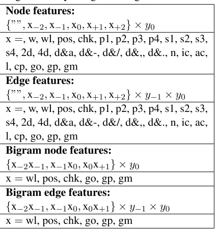
Table 1: Local features used. The value of a node feature is determined from the current label,y0, and a surface feature determined only fromx. The value of an edge feature is determined by the previous la-bel,y₋1, the current label,y0, and a surface feature. Used surface features are the word (w), the down-cased word (wl), the POS tag (pos), the chunk tag (chk), the preﬁx of the word of lengthn (pn), the sufﬁx (sn), the word form features: 2d - cp (these are based on (Bikel et al., 1999)), and the gazetteer fea-tures: go for ORG, gp for PER, and gm for MISC. These represent the (longest) match with an entry in the gazetteer by using IOB2 tags.

Node features:

{””,x₋2,x−1,x0,x+1,x+2} ×y0

x=, w, wl, pos, chk, p1, p2, p3, p4, s1, s2, s3, s4, 2d, 4d, d&a, d&-, d&/, d&,, d&., n, ic, ac, l, cp, go, gp, gm

Edge features:

{””,x₋2,x−1,x0,x+1,x+2} ×y−1×y0 x=, w, wl, pos, chk, p1, p2, p3, p4, s1, s2, s3, s4, 2d, 4d, d&a, d&-, d&/, d&,, d&., n, ic, ac, l, cp, go, gp, gm

Bigram node features:

{x−2x₋1,x−1x0,x0x+1} ×y0 x=wl, pos, chk, go, gp, gm

Bigram edge features:

{x₋2x₋1,x−1x0,x0x+1} ×y−1×y0 x=wl, pos, chk, go, gp, gm

number of updates was not zero even after a large number of iterations in practice. We stopped train-ing when the relative change in these values became less than a pre-deﬁned threshold (0.0001) for at least three iterations.

(7)

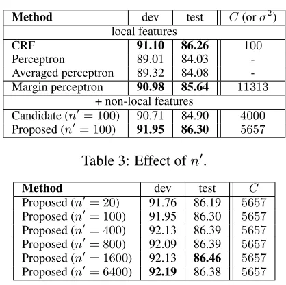
Table 2: Summary of performance (F1).

Method dev test C(orσ2) local features

CRF 91.10 86.26 100

Perceptron 89.01 84.03

-Averaged perceptron 89.32 84.08 -Margin perceptron 90.98 85.64 11313

+ non-local features

Candidate (n′= 100) 90.71 84.90 4000

[image:7.612.80.289.75.283.2]

Proposed (n′= 100) 91.95 86.30 5657

Table 3: Effect ofn′.

Method dev test C Proposed (n′= 20) 91.76 86.19 5657

Proposed (n′= 100) 91.95 86.30 5657

Proposed (n′= 400) 92.13 86.39 5657

Proposed (n′= 800) 92.09 86.39 5657

Proposed (n′= 1600) 92.13 86.46 5657

Proposed (n′= 6400) 92.19 86.38 5657

effects further.

6.2 Results

Table 2 compares the results. CRF outperformed the perceptron by a large margin. Although the av-eraged perceptron outperformed the perceptron, the improvement was slight. However, the margin per-ceptron greatly outperformed compared to the aver-aged perceptron. Yet, CRF still had the best baseline performance with only local features.

The proposed algorithm with non-local features improved the performance on the test set by 0.66

points over that of the margin perceptron without non-local features. The row “Candidate” refers to the candidate algorithm (Algorithm 4.1). From the results for the candidate algorithm, we can see that the modiﬁcation part, (B), in Algorithm 4.2 was es-sential to make learning with non-local features ef-fective.

We next examined the effect of n′. As can be seen from Table 3, an n′ larger than that for train-ing yields higher performance. The highest perfor-mance with the proposed algorithm was achieved when n′ = 6400, where the improvement due to non-local features became0.74points.

The performance of the related work (Finkel et al., 2005; Krishnan and Manning, 2006) is listed in Table 4. We can see that the ﬁnal performance of our algorithm was worse than that of the related work.

[image:7.612.313.545.85.163.2]

We changed the experimental setting slightly to investigate our algorithm further. Instead of

Table 4: The performance of the related work.

Method dev test

Finkel et al., 2005 (Finkel et al., 2005)

baseline CRF - 85.51

+ non-local features - 86.86

Krishnan and Manning, 2006 (Krishnan and Manning, 2006)

baseline CRF - 85.29

[image:7.612.319.534.204.300.2]

+ non-local features - 87.24

Table 5: Summary of performance with POS/chunk tags by TagChunk.

Method dev test C(orσ2) local features

CRF 91.39 86.30 200

Perceptron 89.36 84.35

-Averaged perceptron 89.76 84.50 -Margin perceptron 91.06 86.24 32000

+ non-local features

Proposed (n′= 100) 92.23 87.04 5657 Proposed (n′= 6400) 92.54 87.17 5657

the POS/chunk tags provided in the CoNLL 2003 dataset, we used the tags assigned by TagChunk (Daum´e III and Marcu, 2005)10 with the intention of using more accurate tags. The results with this setting are summarized in Table 5. Performance was better than that in the previous experiment for all al-gorithms. We think this was due to the quality of the POS/chunk tags. It is interesting that the ef-fect of non-local features rose to 0.93 points with

n′ = 6400, even though the baseline performance was also improved. The resulting performance of the proposed algorithm with non-local features is higher than that of Finkel et al. (2005) and compara-ble with that of Krishnan and Manning (2006). This comparison, of course, is not fair because the setting was different. However, we think the results demon-strate a potential of our new algorithm.

The effect of BPM initialization was also exam-ined. The number of BPM runs was 10 in this experiment. The performance of the proposed al-gorithm dropped from91.95/86.30 to91.89/86.03

without BPM initialization as expected in the set-ting of the experiment of Table 2. The perfor-mance of the margin perceptron, on the other hand, changed from90.98/85.64to90.98/85.90 without BPM initialization. This result was unexpected from the result of our preliminary experiment. However, the performance was changed from91.06/86.24to

10

(8)

Table 6: Comparison with re-ranking approach.

Method dev test C

local features

Margin Perceptron 91.06 86.24 32000 + non-local features

Re-ranking 1 (n′= 100) 91.62 86.57 4000 Re-ranking 1 (n′= 80) 91.71 86.58 4000 Re-ranking 2 (n′= 100) 92.08 86.86 16000 Re-ranking 2 (n′= 800) 92.26 86.95 16000 Proposed (n′= 100) 92.23 87.04 5657 Proposed (n′= 6400) 92.54 87.17 5657 Table 7: Comparison of training time (C = 5657).

Method dev test time (sec.) local features

Margin Perceptron 91.04 86.28 15,977 + non-local features

Re-ranking 1 (n′= 100) 91.48 86.53 86,742 Re-ranking 2 (n′= 100) 92.02 86.85 112,138 Proposed (n′= 100) 92.23 87.04 28,880 91.17/86.08 (i.e., dropped for the evaluation set as expected), in the setting of the experiment of Table 5. Since the effect of BPM initialization is not con-clusive only from these results, we need more exper-iments on this.

6.3 Comparison with re-ranking approach

Finally, we compared our algorithm with the re-ranking approach (Collins and Duffy, 2002; Collins, 2002b), where we first generate the n-best candi-dates using a model with only local features (the first model) and then re-rank the candidates using a model with non-local features (the second model). We implemented two re-ranking models, “re-ranking 1” and “re-“re-ranking 2”. These models dif-fer in how to incorporate the local information in the second model. “re-ranking 1” uses the score of the first model as a feature in addition to the non-local features as in Collins (2002b). “re-ranking 2” uses the same local features as the first model11 in addi-tion to the non-local features. The first models were trained using the margin perceptron algorithm in Al-gorithm 3.1. The second models were trained using the algorithm, which is obtained by replacing{yn}

with then-best candidates by the first model. The first model used to generaten-best candidates for the development set and the test set was trained using the whole training data. However, CRFs or percep-trons generally have nearly zero error on the train-ing data, although the first model should mis-label

11

The weights were re-trained for the second model.

to some extent to make the training of the second model meaningful. To avoid this problem, we adopt cross-validation training as used in Collins (2002b). We split the training data into 5 sets. We then trained ﬁve ﬁrst models using 4/5 of the data, each of which was used to generate n-best candidates for the re-maining 1/5 of the data.

As in the previous experiments, we tunedCusing the development set withn′ = 100and then tested other values forn′. Table 6 shows the results. As can be seen, re-ranking models were outperformed by our proposed algorithm, although they also outper-formed the margin perceptron with only local fea-tures (“re-ranking 2” seems better than “re-ranking 1”). Table 7 shows the training time of each algo-rithm.12 Our algorithm is much faster than the re-ranking approach that uses cross-validation training, while achieving the same or higher level of perfor-mance.

7 Discussion

As we mentioned, there are some algorithms simi-lar to ours (Collins and Roark, 2004; Daum´e III and Marcu, 2005; McDonald and Pereira, 2006; Liang et al., 2006). The differences of our algorithm from these algorithms are as follows.

Daum´e III and Marcu (2005) presented the method called LaSO (Learning as Search Optimiza-tion), in which intractable exact inference is approx-imated by optimizing the behavior of the search pro-cess. The method can access non-local features at each search point, if their values can be deter-mined from the search decisions already made. They provided robust training algorithms with guaranteed convergence for this framework. However, a differ-ence is that our method can use non-local features whose value depends on all labels throughout train-ing, and it is unclear whether the features whose val-ues can only be determined at the end of the search (e.g., majority features) can be learned effectively with such an incremental manner of LaSO.

The algorithm proposed by McDonald and Pereira (2006) is also similar to ours. Their tar-get was non-projective dependency parsing, where exact inference is intractable. Instead of using

12

(9)

n-best/re-scoring approach as ours, their method modifies the single best projective parse, which can be found efficiently, to find a candidate with higher score under non-local features. Liang et al. (2006) used n candidates of a beam search in the Collins’ perceptron algorithm for machine transla-tion. Collins and Roark (2004) proposed an approxi-mate incremental method for parsing. Their method can be used for sequence labeling as well. These studies, however, did not explain the validity of their updating methods in terms of convergence.

To achieve robust training, Daum´e III and Marcu (2005) employed the averaged perceptron (Collins, 2002a) and ALMA (Gentile, 2001). Collins and Roark (2004) used the averaged perceptron (Collins, 2002a). McDonald and Pereira (2006) used MIRA (Crammer et al., 2006). On the other hand, we em-ployed the margin perceptron (Krauth and M´ezard, 1987), extending it to sequence labeling. We demon-strated that this greatly improved robustness.

With regard to the local update, (B), in Algo-rithm 4.2, “early updates” (Collins and Roark, 2004) and “y-good” requirement in (Daum´e III and Marcu, 2005) resemble our local update in that they tried to avoid the situation where the correct answer cannot be output. Considering such commonality, the way of combining the local update and the non-local up-date might be one important key for further improve-ment.

It is still open whether these differences are ad-vantages or disadad-vantages. However, we think our algorithm can be a contribution to the study for in-corporating non-local features. The convergence guarantee is important for the conﬁdence in the training results, although it does not mean high per-formance directly. Our algorithm could at least im-prove the accuracy of NER with non-local features and it was indicated that our algorithm was supe-rior to the re-ranking approach in terms of racy and training cost. However, the achieved accu-racy was not better than that of related work (Finkel et al., 2005; Krishnan and Manning, 2006) based on CRFs. Although this might indicate the limita-tion of perceptron-based methods, it has also been shown that there is still room for improvement in perceptron-based algorithms as our margin percep-tron algorithm demonstrated.

8 Conclusion

In this paper, we presented a new perceptron algo-rithm for learning with non-local features. We think the proposed algorithm is an important step towards achieving our ﬁnal objective. We would like to in-vestigate various types of new non-local features us-ing the proposed algorithm in future work.

Appendix A: Convergence of Algorithm 4.2

Letαk_{be a weight vector before the}_k_{th update and}

ϵk be a variable that takes 1 when thekth update is done in (A) and 0 when done in (B). The update rule can then be written asαk+1 =αk+ϵk(Φa∗−Φa+

(1−ϵk)(Φl∗−Φl).13 First, we obtain

αk+1·Ul =αk·Ul+ϵk(Φa∗·Ul−Φa·Ul)

+(1−ϵk)(Φl∗·Ul−Φl·Ul) ≥αk·Ul+ϵkδ+ (1−ϵk)δ

=αk·Ul+δ≥α1·Ul+kδ =kδ

Therefore, (kδ)2 ≤ (αk+1 · Ul)2 ≤ (||αk+1||||Ul||)2 = ||αk+1||2 — (1). On the other hand, we also obtain

||αk+1||2 ≤ ||αk||2+ 2ϵkαk(Φa∗−Φa)

+2(1−ϵk)αk(Φl∗−Φl)

+{ϵk(Φa∗−Φa) + (1−ϵk)(Φl∗−Φl)}2 ≤ ||αk||2+ 2C+R2

≤ ||α1||2+k(R2+ 2C) =k(R2+ 2C)— (2)

We used αk_(Φa∗ ₋_Φa₎ _≤ _Ca_, _αk_(Φl∗ ₋_Φl₎ _≤

Cl andCl = Ca = C to derive 2C in the second inequality. We used||Φl∗−Φl|| ≤ ||Φa∗−Φa|| ≤R

to deriveR2.

Combining (1) and (2), we obtain k ≤ (R2 + 2C)/δ2. Substituting this into (2) gives ||αk|| ≤ (R2_+2C)/δ_{. Since}_y_∗₌_y′_and_Φa∗_·_α₋_Φa′′_·_α_>

Cafter convergence, we obtain

γ′(α) = min xi

Φa∗·α−Φa′′·α

||α|| ≥Cδ/(2C+R

2_).

13

We use the shorthand Φa∗ = Φa(xi,y∗i), Φ a

= Φa(xi,y),Φl∗ = Φl(xi,y∗i), andΦ

l

= Φl(xi,y)wherey

(10)

References

D. M. Bikel, R. L. Schwartz, and R. M. Weischedel. 1999. An algorithm that learns what’s in a name. Ma-chine Learning, 34(1-3):211–231.

R. Bunescu and R. J. Mooney. 2004. Collective infor-mation extraction with relational markov networks. In

ACL 2004.

S. F. Chen and R. Rosenfeld. 2000. A survey of smooth-ing techniques for ME models. IEEE Transactions on Speech and Audio Processing, 8(1):37–50.

M. Collins and N. Duffy. 2002. New ranking algorithms for parsing and tagging: Kernels over discrete struc-tures, and the voted perceptron. In ACL 2002, pages 263–270.

M. Collins and B. Roark. 2004. Incremental parsing with the perceptron algorithm. InACL 2004.

M. Collins. 2002a. Discriminative training methods for hidden Markov models: Theory and experiments with perceptron algorithms. InEMNLP 2002.

M. Collins. 2002b. Ranking algorithms for named-entity extraction: Boosting and the voted perceptron. InACL 2002.

K. Crammer, O. Dekel, J. Keshet, S. Shalev-Shwartz, and Y. Singer. 2006. Online passive-aggressive al-gorithms. Journal of Machine Learning Research.

H. Daum´e III and D. Marcu. 2005. Learning as search optimization: Approximate large margin methods for structured prediction. InICML 2005.

J. R. Finkel, T. Grenager, and C. Manning. 2005. In-corporating non-local information into information ex-traction systems by Gibbs sampling. InACL 2005.

C. Gentile. 2001. A new approximate maximal margin classiﬁcation algorithm.JMLR, 3.

R. Herbrich and T. Graepel. 2000. Large scale Bayes point machines. InNIPS 2000.

W. Krauth and M. M´ezard. 1987. Learning algorithms with optimal stability in neural networks. Journal of Physics A 20, pages 745–752.

V. Krishnan and C. D. Manning. 2006. An effective two-stage model for exploiting non-local dependencies in named entity recognitioin. InACL-COLING 2006.

J. Lafferty, A. McCallum, and F. Pereira. 2001. Con-ditional random ﬁelds: Probabilistic models for seg-menting and labeling sequence data. In ICML 2001, pages 282–289.

Y. Li, H. Zaragoza, R. Herbrich, J. Shawe-Taylor, and J. Kandola. 2002. The perceptron algorithm with un-even margins. InICML 2002.

P. Liang, A. Bouchard-Cˆot´e, D. Klein, and B. Taskar. 2006. An end-to-end discriminative approach to ma-chine translation. InACL-COLING 2006.

R. McDonald and F. Pereira. 2006. Online learning of approximate dependency parsing algorithms. InEACL 2006.

R. McDonald, K. Crammer, and F. Pereira. 2005. Online large-margin training of dependency parsers. InACL 2005.

T. Nakagawa and Y. Matsumoto. 2006. Guessing parts-of-speech of unknown words using global information. InACL-COLING 2006.

L. R. Rabiner. 1989. A tutorial on hidden Markov mod-els and selected applications in speech recognition.

Proceedings of the IEEE, 77(2):257–286.

L. A. Ramshaw and M. P. Marcus. 1995. Text chunk-ing uschunk-ing transformation-based learnchunk-ing. Inthird ACL Workshop on very large corpora.

F. Rosenblatt. 1958. The perceptron: A probabilistic model for information storage and organization in the brain. Psycological Review, pages 386–407.

D. Roth and W. Yih. 2005. Integer linear program-ming inference for conditional random ﬁelds. InICML 2005.

S. Sarawagi and W. W. Cohen. 2004. Semi-Markov ran-dom ﬁelds for information extraction. InNIPS 2004.

L. Shen and A. K. Joshi. 2004. Flexible margin selection for reranking with full pairwise samples. InIJCNLP 2004.

F. K. Soong and E. Huang. 1991. A tree-trellis based fast search for ﬁnding the n best sentence hypotheses in continuous speech recognition. InICASSP-91.

C. Sutton and A. McCallum. 2004. Collective segme-nation and labeling of distant entitites in information extraction. University of Massachusetts Rechnical Re-port TR 04-49.

B. Taskar, C. Guestrin, and D. Koller. 2003. Max-margin Markov networks. InNIPS 2003.