Abstract— Internet users rely on the good capabilities of TCP/IP networks for dealing with congestion. The network delay and the number of users change constantly, which might lead to transmission problems. Usually, these problems are solved following a data communication approach such as drop tail or random early detection (RED) algorithms. Recently, more involved techniques based on an active queue management (AQM) control system have been proposed. This paper presents a probabilistic methodology to test whether a given AQM feedback controller satisfies a predefined set of requirements when dealing with control congestion under a variety of network configurations with a certain degree of confidence. The proposed technique is demonstrated through simulation in NS-2.
Index Terms—Congestion control, controller test, PID, probabilistic analysis.
I. INTRODUCTION
The importance of Internet cannot be denied. Nowadays huge amounts of data are transferred from one point to another in a matter of seconds. However, there are times in which problems arise such as long delays in delivery, lost and dropped packets, oscillations or synchronization problems ([1], [2], [3]). Congestion, which is responsible for many of these problems, appears when there are too many sources sending data too fast for the network to handle and is a very serious problem. Thus, techniques to reduce congestion are of great interest. Nowadays, there are some methodologies to deal with this issue ([4], [5]), such as congestion control, which is used after the network is overloaded, and congestion avoidance, which takes action before the problem appears. This paper deals with congestion control because it is where feedback control techniques can be applied.
The end-to-end transmission control protocol (TCP), and the active queue management (AQM) scheme define the two parts implemented at the routers’ transport layer where congestion control is carried out. The most common AQM objectives ([5], [6] and [7]) are: efficient queue utilization (to minimize the occurrences of queue overflow and underflow, thus reducing packet loss and maximizing link utilization),
Manuscript received January 19, 2010. This work was supported in part by the Junta de Castilla y León under Grant VA037A08 and by the CICYT under grant DPI2007-66718-C04-02.
T. Alvarez and A. Salim are with the Department of Engineering Science and Automatic Control, School of Industrial Engineering, University of Valladolid, Valladolid, Spain (phone: +34 983 423276, email: [email protected], corresponding author). J.M. Maestre And T. Álamo are with the Dept. de Ingeniería de Sistemas yAutomática, Escuela Superior de Ingenieros, University of Seville, Spain (email: pepemaestre, [email protected]).
queuing delay (to minimize the time required for a data packet to be serviced by the routing queue) and robustness (to maintain closed-loop performance in spite of changing conditions).
In general, AQM schemes enhance the performance of TCP, although they have some disadvantages as they do not work perfectly in every traffic situation. Numerous algorithms have been proposed (see [5] for a good survey on the subject). Random early detection (RED) [9] is the most widely used algorithm. It can detect and respond to long-term traffic patterns, but it cannot detect congestion caused by short-term traffic load changes. AQM mathematical models were published in [6], among others. From the moment this paper was known by the control community, control theory based approaches have been used to analyze and design AQM congestion control algorithms and schemes (see references [1] to [20] ).
However, the simulation results (in most of the references) show only specific cases and scenarios. Thus, validation of a control approach from a global point of view is not possible. Nevertheless, in [17] and [18], some theoretical results to ensure stability are portrayed, although they only refer to P and PI controllers. In recent years, research on probabilistic analysis and design methods for systems and control has significantly progressed. Areas such as uncertain and hybrid systems [19] have seen improvements worthy of note. [20] introduces a significant improvement in the sample complexity.
Motivated by these issues, this paper develops a mathematical tool to test whether a set of controllers robustly satisfies a set of predefined requirements with a certain probability. This is a particularization of the method proposed in [21]. One of the main characteristics of the technique is that it is independent of the family of controllers (PI, PID, predictive, robust, etc). As we are applying this technique to the AQM congestion control problem, the main metrics proposed to determine controller performance are: the router queue size (real value and standard deviation), the link utilization and the probability of packet losses.
The proposed technique is applied to a problem of two routers connected in a Dumbbell topology, which represents a single bottleneck scenario. The length of their queues is controlled with a PID whose properties are guaranteed following the results presented in the paper. The simulations are done using the software NS-2 ([28]).
This paper is organized as follows. Section II introduces the theory behind the proposed randomized test method. Results and an example of application are given in section III. Finally, some conclusions and discussion on future work are presented in the last section.
A Method for Testing AQM Controllers with
Probability Guaranteed Properties
II. RANDOMIZED TEST METHOD
In this paper we propose to use a randomized approach to test whether a controller robustly satisfies a set of requirements with a given probabilistic error margin. This approach is based on [21]. The main idea is to test the controller under a finite set of different scenarios. If the controller satisfies the requirements for a sufficient number of these scenarios, then certain properties can be concluded with a given degree of confidence. This section briefly develops the mathematical tools needed to establish a bound on the number of simulations needed to guarantee certain properties with the desired level of confidence probability. A.Notation
Let be a vector representing the parameters that characterize the controller and w W be a vector representing the parameters that characterize the scenario where the controller will work. The concept of scenario includes not only the model for the system under control but also its state and possible inputs.
B.Assumptions
The following assumptions are made for the further results:
I) The controller must belong to a finite family, that is,
has finite cardinality and its number of elements is equal to m:
1, ,...,
2
m
.This assumption is typical in robustness problems, where the controller design parameters, along with different auxiliary variables, are parameterized by means of the decision variable vector
.II) The network and its possible inputs can both be modelled mathematically and these models can be characterized with a parameter vector
w W
.III) Given t1 andt2, witht2t1, a scenario
w W
ˆ
and a controller ˆ , there is a procedure to evaluate whether the controller ˆ fulfils the design requirements during the time interval
t t1, 2
for the scenariow
ˆ
. This procedure returns a 0 if the requirements are satisfied and 1 in any other case. Mathematically, the procedure is a function g such that:
: 0,1
g W .
Remark. This procedure can be based, for example, on a network simulator that checks if the controller being tested fulfils a given set of conditions.
IV) There is a probability distribution PrW defined over the set W and an algorithm that provides elements of W according to
Pr
W. In other words, the algorithm is able to provide a sequence w w1, 2,...,wk of characteristicindependent and identically distributed elements of W obtained according to
Pr
W.Remark. This assumption can be relaxed. It is not strictly necessary to know the probability function
Pr
W if, by somemeans, it is possible to generate the sequence of characteristic elements
w w
1,
2,...,
w
k
W
.C. Problem formulation
The problem is to test whether a controller satisfies the design requirements defined by the function g with a probability greater than
1
, that is:
?
( ) Pr : , 1
g
E w W g w . (1) Notice that
is the probability that the given controller
ˆ does not work properly in a scenario w.In general, it is not possible to test the controller in all of the possible scenarios in order to determine
. We propose to take a probabilistic approach to test a controller. To this end, a finite set of N elements of independent and identically distributed elementsw w
1,
2,...,
w
N
W
are taken accordingto the probability distribution PrW. These scenarios test if the controller satisfies the requirements and allow the probability of failure to be estimated:
1
1 ?
ˆ ( )g N , i i
E g w
N
(2) Whereis a bound of the empirical estimation of the probability of failure for all the controllers being tested. In other words, these parameters set the maximum acceptable probability of failure and can be seen as a design parameter. In the case when a controller exceeds this bound it will be dismissed. Additionally, we will require , that is, the estimated probability of failure must be lower than the real probability of failure
. This constraint means that in practice more restrictive conditions are applied and provides a margin to assure that the real behaviour will fail with less probability than
.The probability that the algorithm fails has to be taken into account. The algorithm fails when it does not provide a solution that satisfies (1), even when it satisfies (2), that is, when a false positive occurs. Thus, the probability of failure of the algorithm is defined as:
? ˆ
Pr Eg( ) Eg( )
Note that, given a controller ˆ, this is a function of
,
and N. Failures in the algorithm are related to situations in which the choice of the characteristic sequence1, 2,..., N
w w w W is not really representative forW.
Logically, the more different scenarios are used to test the controller, the better the results provided by the algorithm. It can be proved that the function of the probability of failure of the algorithm verifies:
lim , , 0
N N
.
As it is not possible to make infinite simulations to guarantee that the probability of failure of the algorithm is 0, we will set a bound ˆ
that represents the maximum algorithm failure rate allowed. In other words, we require
<ˆ.
controller so that it can be guaranteed with a level of confidence ˆ
that the chosen controller works properly according to the design parameters; that is,
, ,N
ˆ. D.Case of one controller under testFor simplicity, it will first be assumed that the controller is the only element in a set of cardinality 1, that is,
ˆ .Without loss of generality; it can be assumed that the
controller verifies:
? ?
( ) Pr : , 1 ,
g
E w W g w ,
that is, the chosen controller fails with probability ˆ for a scenario w W . In other words, we assume that the controller does not fulfil the design requirements in (1). With this assumption, we can calculate the probability that a bad controller has to successfully pass the tests in (2). It is obvious that a controller that fails with
ˆ in (1) has a bigger chance of passing the tests in (2) and therefore this case, the most restrictive one, will be used to establish the bound.When the controller is tested with the N scenarios the goal is to verify (2), which can be transformed into:
1 ˆ, N i ig w N
,where N is N floor rounded. Note that the last inequality is a sufficient condition to guarantee that (2) holds, but it is not equivalent since NN . The probability for this event can be calculated with the aid of the binomial distribution, which is defined as the sum of the probabilities of all the cases where the number of failed scenarios is lower than or equal to N.
1 0
ˆ
Pr , 1
N N N k k i i k N g w N
k
. (3)
This is the probability that sets the bound of confidence in the algorithm, so N has to be chosen such that:
0 ˆ 1 N N k k k N k
. (4)D. General case
In general, several controllers will be tested until one which satisfies the requirements is found. In this case, the number of scenarios that has to be considered to obtain a certain degree of confidence needs to be modified in order to take into account the possibility of choosing a set of non-relevant scenarios for a given controller. Therefore, we assume that the set of tested controllers has a finite cardinality m>1, that is,
1, ,...,2 m
. Assuming thateach of the available controllers has the same probability that was derived in the previous subsection it is easy to derive that N has to be chosen so that:
0 ˆ 1 N N k k k N m k
. (5)Thus, givenˆ,
,
and m, it is possible to establish a number N of representative scenarios that are enough to guarantee that the controller works properly with a confidence level of ˆ. There are several ways to find the value of N that validate (5). For the example in this paper, a numerical bisection method was programmed.Remark. Notice that (5) admits other possible applications. For instance, it can also be used to determine possible probability bounds given a set N of possible simulations and controllers to be tested.
Remark. The finite cardinality assumption holds for cases such as when there is a random number of samples in the space of design parameters according to a given probability ([21]-[23]).
III. TCP/IPNETWORK PROBLEM
This section presents simulation results that demonstrate the method developed in section II. In general, the dynamics of an AQM router are complex due to the number of variables that come into play: packet sources, protocols, etc. Nevertheless, it is possible to obtain a nonlinear model that represents the dynamics of the system [6] considering that the protocol used is TCP. The model relates the average value of the network variables and is described by the following coupled, nonlinear differential equations:
1 ( ) ( ( ( )))
( ) ( ( ))
( ) 2 ( ( ))
( )
( ), 0
( ) ( )
( )
max 0, ( ) , 0
( )
TCP
TCP
W t W t R t R t
W t p t R t
R t R t R t
N t
C W t q
R t q t
N t
C W t q
R t
, (6)
where W ≈ average TCP window size (packets),
q average queue length (packets), R ≈round-trip time = q/C+Tp (secs), C ≈ link capacity (packets/sec), Tp ≈
propagation delay (secs), NTCP ≈ load factor (number of
TCP sessions) and p ≈ probability of packet mark. As explained by [6], the first differential equation in (6) describes the TCP window control dynamic and the second equation models the bottleneck queue length as an accumulated difference between the packet arrival rate and the link capacity. The queue length and window size are positive, bounded quantities, i.e., q
0,q andW
0,W , where q and W denote buffer capacity and maximum window size, respectively. In this formulation, the congestion window size W(t) is increased by one every round-trip time if no congestion is detected, and is halved when congestion is detected.Although an AQM router is a non-linear system, in order to analyze certain types of properties and design controllers, a linearized model was used. To linearize (6), we assume that the number of active TCP sessions and the link capacity are constant, i.e., NTCP(t)=NTCPand C(t)=C. The dependence of
the time delay argument t−R on queue length q is ignored and it is assumed to be fixed to t−R0. Then, local linearization of
(6) around the operating point results in the following equation:
0 2 0 2 0 0 0 2 2 0 ( ) ( ) ( ) 1 ( ) ( ) ( ) 2 TCP TCP NW t W t W t R
R C
R C
q t q t R p t R
R C N
) ( 1 ) ( ) ( 0 0 t q R t W R N t
q
, (7)
where W(t)WW0, qqq0 and p pp0 ,
represent the perturbed variables. The operating point for a desired equilibrium queue length q0 is given by:
p
T C q R 0
0 , 0 0 TCP R C W N and 2 0 0 2 W
p . (8) Equation (2) can be further simplified by separating the low frequency (‘nominal’) behavior (P(s) in (4)) of the window dynamic from the high frequency behavior (∆(s) in (9)) which is accounted as a parasitic.
2 2 0 0 (2 ) ( ) ,(2 ) ( ) 1
TCP
TCP C N P s
s N R C s R
0
2 3 0
2
( )s NTCP 1 e R s R C
(9) Taking (9) as a starting point, [6] provides a feedback control system of AQM (Fig. 1).
The action implemented by an AQM control law is to mark packets with a discard probability p, as a function of the measured queue length q. The larger the queue, the greater the discard probability becomes. Following (9), the transfer function Δ(s) denotes the high-frequency window dynamics and P(s) (plant dynamics) relates how p dynamically affects q.
The controller used for the simulations was a PID [27], which is the most common form of feedback. It can be described by (8):
t di p dt t de T d e T t e K t u 0
[image:4.595.310.548.64.213.2]1 (10)
Figure 1: Block diagram of AQM as feedback control system
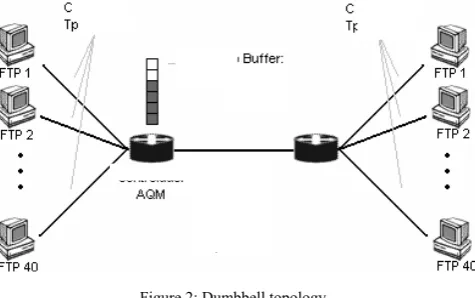
Figure 2: Dumbbell topology
Equation (10) represents the classic or textbook formulation, but as we are going to implement the controller in a computer some practical issues should be taken into account. Following [27], the discrete equations implemented in the software network simulator 2 (NS-2) are given by (11).
1 1 1 , , , ,k p k
d
k k p TCP k k
d TCP s
k k k k
p
k k k
i p t K e t
T
d t d t K N y t y t T N T
u t sat p t d t i t
K t i t e t
T
(11)
where NTCP is a value between 8 and 20 and Ts is the
sampling period. This controller is very well known to the control community. Its parameters can be tuned following methods proposed in the control literature such as Ziegler-Nichols reaction curve. The block diagram is the same as in Figure 2.
The basic network topology used as the example to test the controller is depicted in Figure 2. It is a typical single bottleneck topology and reflects the working scenario defined in [16]: NTCP=40 TCP sessions, C = 250 packets/sec.,
Tp=0.3 sec., so R0=0.7 and W0= 4.375 packets. These are the
nominal conditions, although fluctuations are possible. The following reasonable changes in the conditions of the experiment have been considered: the number of TCP sessions can fluctuate between 20 and 180, the link capacity between 100 and 1000 packets/sec and the transportation delay Tp, between 0.1 and 0.6 seconds.
[image:4.595.52.292.607.727.2]0
50
100
150
200
250
300
0
100
200
q: mean
0
50
100
150
200
250
300
0
100
200
N
0
50
100
150
200
250
300
0
500
1000
C
0
50
100
150
200
250
300
0
0.5
1
p: mean
0
50
100
150
200
250
300
0
50
100
[image:5.595.78.517.54.734.2]q: std
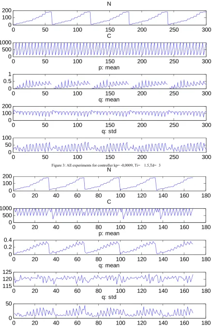
Figure 3: All experiments for controller kp= -0,0009, Ti= 1.5,Td= 3
0
20
40
60
80
100
120
140
160
180
115
120
125
q: mean
0
20
40
60
80
100
120
140
160
180
0
100
200
N
0
20
40
60
80
100
120
140
160
180
0
500
1000
C
0
20
40
60
80
100
120
140
160
180
0
0.2
0.4
p: mean
0
20
40
60
80
100
120
140
160
180
0
50
q: std
20 25 30 35 40 45 50 55 60 65 70 80
100 120 140 160
20 25 30 35 40 45 50 55 60 65 70
80 100 120 140 160
20 25 30 35 40 45 50 55 60 65 70
[image:6.595.347.515.586.672.2]80 100 120 140 160
Figure 5: Simulation results
Thus, we have a total of 54 possible controllers. The simulations will be satisfactory if the queue size, whose reference will be at 120 packets, has a mean value in the interval [116, 124] and its mean deviation is smaller than 17. These are the bounds that define the function g introduced in section II. The procedure consists in testing one controller after another until one is found that fulfills the design requirements. The number of samples needed to test each controller depends on the number of controllers being tested. For example, if controller 1 fails then controller 2 and controller 1 are put to the test with a bigger number of scenarios. This is repeated until a controller that fulfills all the requirements is obtained.
To this end, (5) was used to establish the desired properties for the controllers, fixing the following parameters:
0.05, that is, we admit that the controller may not fulfil, in 5% of the cases, the criteria used in the testing algorithm proposed in Section 2.
0.01, that is, for each 100 scenarios simulated, only one failure is tolerated. A failure here means that the controller being tested has not achieved the required performance in the chosen metric for a given simulation scenario.
ˆ0.1, that is, a maximum of 10% of the scenarios may not be valid (repeated simulations, non realistic scenarios, etc).
m=54, that is, 54 different controllers are considered to be tested.
In this case, (5) is used to establish the number of required simulations for each controller, so that the desired properties can be statistically guaranteed. As we are interested in finding the best possible controller within the
given set, all of them are put to the test and the one that offers the best results is kept. In our experiments, the resulting number of different scenarios needed to obtain a successful controller was 168 simulations. Notice that, with an increment in the number of simulations, the probability bounds could also be improved.
Remark. In the case that none of the controllers should pass the simulation tests, the requirements would have to be relaxed or the controlling scheme changed.
After the simulations finished, it can be concluded that the controller with kp= -0,0009, Ti=1.5 and Td=3 successfully passed the tests: therefore its performance is statistically guaranteed within the range established. Figs. 3 and 4 show, respectively, all the scenarios and the ones that passed the specifications, for the selected controller (the one that fulfills the initial performance specifications).
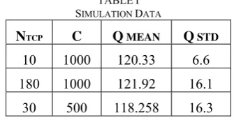
TABLEI SIMULATION DATA
NTCP C Q MEAN Q STD
10 1000 120.33 6.6 180 1000 121.92 16.1 30 500 118.258 16.3
IV. CONCLUSIONS
A methodology to statistically guarantee the properties of a family of controllers has been presented in this paper. The proposed method does not depend on the family of controllers considered, as it is very flexible. For instance, it can be used to determine probability bounds or establish a minimum number of simulations required to accept or reject a controller.
The importance of this result yields, in fact, that it allows some properties to be guaranteed with a given probability level in cases where there is a great difficulty, or even an impossibility, to demonstrate the cited properties. This is especially useful in this area, as it is common to find design procedures in the literature that are only tested in a few cases with no guarantee that the controller behavior will be similar in other scenarios.
ACKNOWLEDGMENT
Authors thank Prof. F. Tadeo for so many fruitful discussions.
REFERENCES
[1] Azuma, T., T. Fujita, M. Fujita (2006). Congestion control for TCP/AQM networks using State Predictive Control. Electrical Engineering in Japan, 156, 1491-1496.
[2] Xiong, N., Y. He, Y. Yang, B. Xiao, X. Jia (2005). On designing a novel PI controller for AQM routers supporting TCP flows. APWEB 2005, 991-1002.
[3] Deng, X., S. Yi, G. Kesidis. C.R. Das (2003). A control theoretic approach for designing adaptive AQM schemes. GLOBECOM’03,
5, 2947 – 2951.
[4] Jacobson, V. (1988). Congestion avoidance and control. ACM SIGCOMM’88.
[5] Ryu, S., C. Rump, C. Qiao (2004). Advances in Active Queue Management (AQM) based TCP congestion control. Telecommunication Systems, 25, 317-351.
[6] Hollot, C.V., V. Misra, D. Towsley, W. Gong (2002). Analysis and Design of Controllers for AQM Routers Supporting TCP flows. IEEE Transactions on Automatic Control, 47, 945-959.
[7] Hayes. M.J., S.M. Mahdi Alavi, P. Van de Ven (2007). An Improved Active Queue Management scheme using a two-degree-of-freedom feedback controller. European Control Conference (ECC 2007), July 2-5, 2007, Kos, Greece.
[8] Sun, J., S. Chan, K.-T. Ko, G. Chen, M. Zukerman (2007). Instability effects of two-way traffic in a TCP/AQM system. Computer Communications, 30, 2172-2179.
[9] Floyd, S., V. Jacobson (1993). Random early detection gateways for congestion avoidance. IEEE/ACM Transactions on Networking, 1,
397-413.
[10] Athuraliya, S., S.H. Low, V.H. Li, Q. Yin (2001). REM: active queue management. IEEE Networking, 15, 48-53.
[11] Kelly, F. (2001). Mathematical Modeling of the Internet, in Mathematics Unlimited-2001 and beyond, B. Enquist and W. Schmid, Eds, Berlin, Germany, Springer-Verlag.
[12] Misra, V., W.B. Gong, D. Towsley (2000). Fluid Based Analysis of a network of AQM routers supporting TCP flows with an application to RED. ACM/SIGCOMM 2000, 151-160.
[13] Pagano, M., R. Secchi (2004). A survey on TCP performance evaluation and modelling. Proc. of Int'l Working Conf. on Performance Modelling and Evaluation of Heterogeneous Networks (HET-NET 2004), Ilkley, UK.
[14] Sun, J., M. Zukerman and M. Palaniswami (2007). Stabilizing RED using a fuzzy controller. Proc. Of ICC’07, Glasgow, United Kingdom.
[15] Durresi, A., P. Kandikuppa, M. Sridharan, S. Chellappan, L. Barolli, R. Jain (2006). LED: Load Early Detection: A Congestion Control Algorithm based on Router Traffic Load. Journal of Information Processing Society of Japan, 47, 94 – 107.
[16] Quet, P.-F., H. Özbay (2004). On the design of AQM supporting TCP flows using robust control theory. IEEE Transactions on Automatic Control, 49, 1031-1036.
[17] Al-Hammouri, A.T., V. Liberatore, M.S. Branicky and S.M. Phillips (2006). Complete stability region characterization for PI-AQM. ACM SIGBED Review, 3, 1-6.
[18] Aweya, J., M. Ouelette, D.Y. Montuno and K. Felske (2008). Design of rate-based controllers for active queue management in TCP/IP networks. Computer Communications, 31, 3344-3359.
[19] R. Tempo, G. Calafiore and F. Dabbene. Randomized Algorithms for Analysis and Control of Uncertain Systems. Communication and Control Engineering Series. Springer-Verlag, London, 2005. [20] T. Alamo, R. Tempo and E. F. Camacho. Randomized strategies for
probabilistic solutions of uncertain feasibility and optimization problems. IEEE Transactions on Automatic Control, accepted for publication, 2009.
[21] T. Alamo, R.Tempo and A. Luque. On the sample complexity of probabilistic analysis and design methods. Perspectives in Mathematical System Theory, Control and Signal Processing. Lecture Notes in Control and Information Sciences. Springer, accepted for publication 2010.
[22] Y. Fujisaki and Y. Kozawa. Probabilistic robust controller design: probable near minimax value and randomized algorithms. Probabilistic and Randomized Methods for Desigh under Uncertainty. Springer, London 2006.
[23] M. Vidyasagar. Randomized algorithms for robust controller synthesis using statistical learning theory. Automatica, 37:1515-1528,2001.
[24] T. Alvarez and S. Cristea, AQM Control of TCP/IP Networks using Generalized Predictive Control, in Proc. UKACC International Conference on Control 2008, Manchester, UK, Sep 2-4, 2008. [25] Ramakrishnan, K., S. Floyd (1999). Explicit Congestion
Notification. ACM SIGCOMM Computer Communications Review,
24, 8-23.
[26] .EcosimPro. The El Modelling language. www.ecosimpro.com. [27] K. J. Aström and T. Hägglund, Advanced PID control. ISA. NC,
2006.
[28] Network Simulator, NS-2, http:/www.isi.edu/nsnam/ns/
[29] W.-K. Chen, Linear Networks and Systems (Book style). Belmont, CA: Wadsworth, 1993, pp. 123–135.
[30] Comer, Douglas E. (2006). Internetworking with TCP/IP, 5, Prentice Hall: Upper Saddle River, NJ.
[31] G. O. Young, “Synthetic structure of industrial plastics (Book style with paper title and editor),” in Plastics, 2nd ed. vol. 3, J. Peters, Ed. New York: McGraw-Hill, 1964, pp. 15–64.
[32] W.-K. Chen, Linear Networks and Systems (Book style). Belmont, CA: Wadsworth, 1993, pp. 123–135.
[33] H. Poor, An Introduction to Signal Detection and Estimation. New York: Springer-Verlag, 1985, ch. 4.
[34] B. Smith, “An approach to graphs of linear forms (Unpublished work style),” unpublished.
[35] E. H. Miller, “A note on reflector arrays (Periodical style—Accepted for publication),” IEEE Trans. Antennas Propagat., to be published.
[36] J. Wang, “Fundamentals of erbium-doped fiber amplifiers arrays (Periodical style—Submitted for publication),” IEEE J. Quantum Electron., submitted for publication.
[37] C. J. Kaufman, Rocky Mountain Research Lab., Boulder, CO, private communication, May 1995.
[38] Y. Yorozu, M. Hirano, K. Oka, and Y. Tagawa, “Electron spectroscopy studies on magneto-optical media and plastic substrate interfaces(Translation Journals style),” IEEE Transl. J. Magn.Jpn., vol. 2, Aug. 1987, pp. 740–741 [Dig. 9th Annu. Conf. Magnetics
Japan, 1982, p. 301].
[39] M. Young, The Techincal Writers Handbook. Mill Valley, CA: University Science, 1989.
[40] (Basic Book/Monograph Online Sources) J. K. Author. (year, month, day). Title (edition) [Type of medium]. Volume(issue). Available: http://www.(URL)
[41] J. Jones. (1991, May 10). Networks (2nd ed.) [Online]. Available: http://www.atm.com
[42] (Journal Online Sources style) K. Author. (year, month). Title. Journal [Type of medium]. Volume(issue), paging if given. Available: http://www.(URL)