Abstract — This paper proposes optimization measures for assessing compromise solutions in multi-response problems that have been formulated in the Response Surface Methodology framework. The measures take into account the desired properties of responses at optimal variable settings, namely, the bias, quality of predictions and robustness, providing relevant information to the analyst that allows achieving solutions of interest and feasible in practice. Two examples from the literature show the utility of the proposed measures.
Index Terms —Desirability, Loss function, Variance, Response Surface, Robustness.
I. INTRODUCTION
Optimization theory is a research field that has been expanding in all areas of applied mathematics, engineering, medicine, economics and other sciences at an astonishing rate during the last few decades. New algorithms and methodologies have been developed and its diffusion into various disciplines has proceeded at a rapid pace. To date, researchers are paying great attention to hybrid approaches to avoid premature algorithm convergence toward a local maximum or minimum and reach the global optimum in problems with multiple objectives [1]. The issue is that the level of computational and mathematical or statistical expertise required for using those algorithms or methodologies and solving such problems successfully is significant. This makes such sophisticated tools hard to adopt, in particular, by practitioners [2]-[3].
A strategy widely used for optimizing multiple objectives (multiresponses) in the Response Surface Methodology (RSM) framework consists of converting the multiresponses into a single (composite) function followed by its optimization, using either the generalized reduced gradient or sequential quadratic programming algorithms available in the popular Microsoft Excel® (solver add-in) and Matlab® (fmincon routine), respectively. To form that composite function, the desirability function-based and loss function-based methods are the most popular among practitioners.
The existing methods use distinct composite functions to provide indication about how close the response values are
Manuscript received April 15, 2010.
Nuno Costa, UNIDEMI, Escola Superior de Tecnologia de Setúbal, Campus do IPS, Estefanilha, 2910-761 Setúbal, Portugal (e-mail: [email protected]). Zulema Lopes Pereira, UNIDEMI, Faculdade de Ciências e Tecnologia - Universidade Nova de Lisboa, Monte de Caparica, Portugal ([email protected]). Martin Tanco, CITEM, Universidad de Montevideo, Luis P. Ponce 1307, 11300 Montevideo, Uruguay ([email protected]).
from their target. However, those functions may give different values for the same solution, which is a relevant shortcoming as may confound the analyst and make difficult the task of assigning priorities (weights) to responses. So, this paper aims at proposing optimization performance measures with a threefold purpose:
I. Provide relevant information to the analyst so that he/she may achieve compromise solutions of interest if an optimization method which does not consider the responses’ variance level and responses’ correlation information is used;
II. Help the analyst in evaluating the feasibility of a compromise solution by assessing its bias (responses deviation from their target), quality of predictions (variance of the predicted responses) and robustness (variance due to uncontrollable variables) separately; III. Allow evaluating the method’s solutions that cannot be
compared directly due to the different approaches subjacent to those methods, for example, loss function-based and desirability function-function-based methods.
The remainder of the paper is organized as follows: the following section presents a review of the selected methods. Then optimization measures are proposed. The next section includes two examples from the literature to show the usefulness of the optimization measures. The subsequent section discusses the results. Conclusions are presented in the last section.
II. METHODS REVIEW
The variety of real-life problems requiring the consideration of multiple objectives and practitioners’ desire to propose enhanced techniques using recent advancements in mathematical optimization, scientific computing and computer technology make the multiresponse optimization an active research field. A review on existing methods for simultaneous optimization of multi-responses in the RSM framework, which is thoroughly discussed by Myers et al. [4]-[5], is provided in [6]-[7]. Fogliato [8] provides an extensive list of references grouped according to methods theoretical framework. In practice, the desirability based and loss function-based methods are the most popular among practitioners who look for optimum variable settings for the process and product while considering multiple responses simultaneously.
A. Desirability-based methods
The desirability-based methods are easy to understand,
Optimization Measures for Assessing
Compromise Solutions in Multiresponse Problems
flexible for incorporating the decision-maker’s preferences (priority to responses), and the most popular of them, the so-called Derringer and Suich’s method [9], or modifications of it [10], is available in many data analysis software packages. However, to use this method the analyst needs to specify the values of four shape parameters (weights). This is not a simple task and makes an impact on the optimal variable settings [11]. To surmount this and other limitations, in [12] is proposed an alternative method that, under the assumptions of normality and homogeneity of error variances, requires minimum information from the user. That desirability-based method, proposed by Cheng et al. [12], is very easy to understand and implement in the readily available Microsoft Excel-Solver tool and, in addition, requires less cognitive effort from the analyst. The user only has to assign values to one type of shape parameters (weights), which is a relevant advantage over the extensively used Derringer and Suich’s method.
Ch’ng et al. [12] suggested individual desirability functions of the form
c y m L U L L U y L U L U yd
2ˆ 1 2ˆ 2 ˆ (1)
where 0d2 and yˆ represents the response´s model with upper and lower bounds defined by U and L, respectively. The global desirability (composite) function is defined as
p d
d e
D p
i i i i i
1 () (2)
where di
i is the value of the individual desirability function i at the target value i, ei is the weight (degree of importance or priority) assigned to response i, p is the number of responses and
p
i 1ei 1. The aim is to minimize D.
Although Ch’ng et al. illustrate their method only for Nominal-the-Best (NTB) response type, in this paper the Larger-the-Best (LTB) and Smaller-the-best (STB) response types are also considered. In these cases, di
Ui and di
Li are used in Equation 2 instead of di
i , under the assumption that it is possible to establish specification limits U and L to those responses. Note that Ch’ng et al.’s method neither considers the quality of predictions nor the robustness.B. Loss function-based methods
The loss function approach uses a totally different idea about the multi-response optimization by considering monetary aspects in the optimization process, and is very popular among the industrial engineering community. Unlike the above-mentioned desirability-based methods, there are loss function-based methods that consider the responses’ variance level and exploit the responses’ correlation information, which is statistically sound. Examples of those methods were introduced in [13]-[14].
Vining [13] proposed a loss function-based method that allows specifying the directions of economic importance for the compromise optimum, while seriously considering the variance-covariance structure of the expected responses. This method aims at finding the variable settings that minimize an expected loss function defined as
y TC E y x trace C xx y E x y L
E ˆ( ), ˆ( ) ˆ( ) ˆ( )
(3) where
yˆ(x)is the variance-covariance matrix of thepredicted responses at x and C is a cost matrix related to the costs of non-optimal design. If C is a diagonal matrix then each element represents the relative importance assigned to the corresponding response. That is, the penalty (cost) incurred for each unit of response value deviated from its optimum. If C is a non-diagonal matrix, the off-diagonal elements represent additional costs incurred when pairs of responses are simultaneously off-target. The first term in Equation 3 represents the penalty due to the deviation from the target; the second term represents the penalty due to the quality of predictions.
Lee and Kim [14] put emphasis on reducing bias and improving robustness. They proposed minimizing an expected loss defined as
p i p i i j j j i i ij ij i i ii y c y y
c x y L E 1 2 1 1 2
2 ˆ ˆ (ˆ )(ˆ )
) ˆ ( )] ), ( ( [ (4) where
c
i andc
ij represent loss coefficients,
ˆ
i2 and
ˆ
ij are elements of the response’s variance-covariance matrix at xy x)
( ( ) . Note that the key difference between Equations 3
and 4 is that the later uses the variance-covariance structure of the responses rather than the variance-covariance structure of the predicted responses.
III. MEASURES OF OPTIMIZATION PERFORMANCE
To evaluate the feasibility of compromise solutions in multiresponse problems, the analyst needs to have information about the solution’s properties at “optimal” variable settings, namely, the bias and variance. In fact, responses at some variable settings may have considerable variance due to the uncertainty in the regression coefficients of predicted responses and sensitivity of responses to uncontrollable variables.
and Xu et al. [16]. While in [14]-[15] the terms or components of the objective function are used for comparing the results of loss function-based methods in terms of the desired response’s properties, in [16] several optimization performance measures to compare only the bias of methods built on different approaches are used. The optimization measures used in [14]-[15] require the definition of a cost matrix, which is not easily defined or readily available. The shortcoming in the optimization measures used in [16] is that they do not consider the response’s dimension and type. In fact, for comparing method’s results it is necessary considering the responses’ dimension, responses’ type and the statistical properties of methods used. Multi-response optimization methods may differ in terms of statistical properties and optimization schemes so the comparison of method´s solutions in a straightforward manner may not be possible. Moreover, each method has its own merits and how good its solution is may depend on either economical and technical issues or decision-maker’s preference. In practice, divergent interests lead to different evaluations of method’s solution so the responses’ dimension and type cannot be ignored.
With the aim at providing useful information for analyst or decision-maker concerning to response’s properties, three optimization measures are suggested to assess those properties separately. The measures can guide the analyst during the optimization process and to help him/her in achieving a solution of interest, even if quality of predictions and robustness are important issues in practice. Moreover, they may also serve to evaluate the solutions obtained from different methods and help the practitioner in making a more informed decision when he/she is interested in choosing a method for optimizing multiple responses.
To assess the method’s solutions in terms of bias we suggest an optimization measure that considers the response types, response’s specification limits and deviation of all responses from their target. This measure, named cumulative bias (Bcum), is defined as
p
i i i i
cum W y
B
1 *
ˆ (5)
where yˆi* represents the estimated response value at “optimal” variable settings and W is a parameter that takes into account the specification limits and response type. This parameter is defined as follows: W 1/(U L) for STB- and LTB-type responses; W 2/(UL) for NTB type responses.
The cumulative bias gives an overall result of the optimization process instead of focusing on the value of a single response, what avoids making unreasonable decisions in some cases [17]. To control the bias of each response, the practitioner may use the individual bias (Bi) defined as
i i i i Wy
B ˆ* (6)
As Bi and Bcum are dimensionless, analyst does not have to
worry with dimensional consistency of responses. These
measures take values greater than or equal to zero, but the most favorable is the zero value.
To assess method’s solutions in terms of quality of predictions is proposed a measure defined as
j T
T
j X Q X x x
trace
QoP 1 1 (7)
where xj is the subset of independent variables consisting of
the Kx1 vector of regressors for the i-th response with N observations on Ki regressors for response, X is an NpxK block
diagonal matrix and QN. An estimate of is
N e e j
T j ij ˆ ˆ /
ˆ
, where ê is the residual vector from the OLS; IN
is an identity matrix and represents the Kronecker product. To make dimensionless when responses are in different units, this matrix is multiplied by matrix , whose diagonal and non-diagonal elements are defined as ii1/(UiLi)2, and ij1/(UiLi)(UjLj), respectively.
Note that QoP is defined under the assumption that Seemingly Unrelated Regression (SUR) method is employed to estimate the regression models (response surfaces) as it yields regression coefficients at least as accurate as those of other popular regression techniques, namely the ordinary and generalized least squares [18]-[19].
The measure for assessing the method’s solutions in terms of robustness is defined as
Rob = trace
y(x)
(8)
where y(x) represents the variance-covariance matrix of the (true) responses. Note that replications of the experimental runs are required for assessing the solution’s robustness and the lower Rob value is, the lower the response’s variance will be.
IV. EXAMPLES
Two examples from the literature illustrate the utility of the proposed performance measures. The first one considers a case study where the quality of prediction is the adverse condition. In this example the methods proposed by Ch’ng et al. [12] and Vining [13] are used. In the second one the adverse condition is the robustness, and the methods proposed by Ch’ng et al. [12] and Lee and Kim [14] are used.
Example 1: The responses specification limits and targets for the percent conversion (y1) and thermal activity (y2) of a polymer are the following: yˆ180.00 with U11100;
00 . 60 ˆ 00 .
55 y2 with 257.50. Reaction time (x1),
reaction temperature (x2), and amount of catalyst (x3) are the
682 . 1 682 .
1
xi , was run to generate the data. The predicted responses for the responses by using SUR method are as follows:
1
ˆ
y = 81.09 + 1.03x1 + 4.04x2 + 6.20x3 - 1.83x12 + 2.94x22 - 5.19x32 + 2.13x1x2 + 11.38x1x3 - 3.88x2x3
2
ˆ
y = 59.85 + 3.58x1 + 0.25x2 + 2.23x3 - 0.83x12 + 0.07x22 - 0.06x32 - 0.39x1x2 - 0.04x1x3 + 0.31x2x3
The model of the thermal activity includes some insignificant regressors (x2, x12, x22, x32, x1x2, x1x3, x2x3), so the predicted response has a poor quality of prediction. This means that thermal activity will have a variance as larger as farther from the origin the variable settings are. The variance-covariance matrix is estimated as
55 . 1 55 . 0 55 . 0 12 . 11 ˆ .
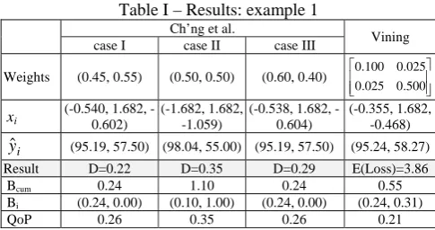
Regarding the results, Table I shows that the global desirability function (D) yields different values for the same response values (cases I and III). This is not desirable or reasonable and may confound analysts who are focused on D value for making decisions. In contrast, the Bcum remains
unchanged, as it is expectable in these instances. By using Bcum
the analyst can easily perceive whether the changes he/she made in the weight values are either favorable or unfavorable in terms of response values. When Bcum increases, this means
that the value of some response(s) is, undesirably, farther from its target, as it is the case of yˆ2 in the Vining’s solution.
In terms of QoP the differences between cases I and III are negligible. Case II serves to illustrate that the analyst can distinguish solutions with larger variability from other(s) with smaller variability looking at QoP value. A small difference exists between Vining’s solution and both cases I and III, because x1 and x2 values are closer from the origin in Vining’s
solution.
This example shows that the proposed measures give better indications (results, information) to the analyst and can help him/her in achieving feasible solutions even if the quality of predictions is an adverse condition.
Example 2: Lee and Kim [14] assumed that the fitted response functions for process mean, variance and covariance for two quality characteristics are as follows:
1
ˆ
y = 79.04 + 17.74x1 + 0.62x2 + 14.79x3 - 0.70x12 - 10.95
2 2
x - 0.10x23 - 5.39x1x2 + 1.21x1x3 - 1.79x2x3
1
ˆ
= 4.54 + 3.92x1 + 4.29x2 + 1.66x3 + 1.15x12 + 4.40x22 + 0.94x32 + 3.49x1x2 + 0.74x1x3 + 1.19x2x3
2
ˆ
y = 400.15 - 95.21x1 - 28.98x2 - 55.99x3 + 20.11 2 1
x +
26.80x22 + 10.91x32 + 57.13x1x2 - 3.73x1x3 - 10.87x2x3
2
ˆ
= 26.11 - 1.34x1 + 6.71x2 + 0.37x3 + 0.77 2 1
x + 2.99x22
-0.97x32 - 1.81x1x2 + 0.41x1x3
12
ˆ
[image:4.595.305.548.186.314.2] = 5.45 - 0.77x1 + 0.16x2 + 0.49x3 - 0.42x12 + 0.50x22 - 0.35x32 - 0.63x1x2 + 1.13x1x3 - 0.30x2x3
Table I – Results: example 1
Ch’ng et al.
Vining case I case II case III
Weights (0.45, 0.55) (0.50, 0.50) (0.60, 0.40)
500 . 0 025 . 0 025 . 0 100 . 0 xi
(0.540, 1.682, -0.602)
(-1.682, 1.682, -1.059)
(0.538, 1.682, -0.604)
(-0.355, 1.682, -0.468)
i
yˆ (95.19, 57.50) (98.04, 55.00) (95.19, 57.50) (95.24, 58.27)
Result D=0.22 D=0.35 D=0.29 E(Loss)=3.86
Bcum 0.24 1.10 0.24 0.55
Bi (0.24, 0.00) (0.10, 1.00) (0.24, 0.00) (0.24, 0.31)
QoP 0.26 0.35 0.26 0.21
In this example it is assumed that the response’s specifications are yˆ160 with U11100 and yˆ2500
with L22300, subject to 1xi1.
Regarding the results, Table II shows that the loss function proposed by Lee and Kim yields different expected loss values for similar solutions (cases I and II). In contrast, the Bcum value
remains unchanged in similar solutions, namely in case I, II and Ch’ng et al.’s solution, confirming its utility for assessing compromise solutions for multi-response problems apart from the method used. Case III serves to illustrate that the analyst can recognize solutions with larger variability due to uncontrollable factor (case III) from others more robust (case I, II and Ch’ng et al.’s solution) looking at Rob value. Note that Ch’ng et al.’s method yields a solution similar to both cases I and II when appropriate weights are assigned to yˆ2 and ˆ2, remaining unchanged (equal to 0.25) the weights for
1
ˆ
y and ˆ1.
This example confirms that the proposed measures give better information to the analyst and can help him/her in achieving feasible solutions even if the robustness is an adverse condition.
Table II – Results: example 2
Lee and Kim
Ch’ng et al.
case I case II Case III
Weights (1, 1, 1) (0.3, 0.5, 0.02) (0.8, 0.3, 0.1) (0.25, 0.25, 0.15, 0.35) xi (0.79, -0.76, 1.00) (0.80, -0.77, 1.00)
(1.00, 1.00, -0.43)
(0.80, -0.75, 1.00)
i
yˆ (97.86, 301.40) (98.06, 300.32) (74.22, 346.45) (98.18, 300.00)
Var-cov (7.80, 22.96, 6.39) (7.84, 22.98, 6.39) (5.98, 23.12, 4.35) (7.86, 22.99, 6.38) Result E(Loss)=598.1 E(Loss)=283.7 E(Loss)=3395.8 D=0.53
Bcum 1.76 1.75 2.39 1.75
Bi
(0.05, 0.78, 0.01, 0.92) (0.05, 0.78, 0.00, 0.92) (0.64, 0.59, 0.23, 0.92) (0.05, 0.79, 0.00, 0.92)
V. DISCUSSION
As noted in [21], the optima are stochastic by nature, and understanding the variability of the true and predicted responses is a critical issue for the practitioners. Thus, the assessment of the responses’ variance level and correlation information separately, in addition to the variance of expected responses at “optimal” variable settings, provide the required information for the analyst evaluating a compromise solution for multi-response optimization problems.
The previous examples show that the expected loss and desirability functions give erroneous information to the analyst, because those measures yield different results in cases where the solutions are equal or have slightly changes in the response values. This is a relevant shortcoming, which is due to the different weights or priorities assigned to responses that are considered in the composite function. In practice, if the analyst only focuses on the result of the composite function used for making decisions he/she may ignore a solution of interest or be confounded about the directions for changing weights or priorities to responses due to that erroneous information. By using the proposed measures the analyst does not have to worry with the reliability of the information as they do not depend on priorities assigned to responses. By this reason, the proposed measures may also serve to compare the performance of methods that use different approaches, for example, between desirability function-based methods and loss function-based methods, and between methods structured under the same approach but that use different composite functions, as it is the case of Derringer and Suich’s method, where the composite function is a multiplicative function, and Ch’ng et al.’s method, where the composite function is an additive function.
From a theoretical point of view, methods that consider the responses’ variance level and exploit the responses’ correlation information may lead to solutions that are more realistic when the responses have either significantly different variance levels or are highly correlated [15]. However, the previous examples show that the proposed measures can provide useful information to the analyst so that he/she achieves compromise solutions with desirable properties at “optimal” settings by using methods that consider or do not consider the variance-covariance structure of responses. Nevertheless, note that points in non-convex response surfaces cannot be captured by weighted sums like those represented by the objective functions of the methods reviewed in this paper. Messac et al. [22] present theoretical details on this issue.
VI. CONCLUSIONS
Low bias and minimum variance are desired response’s properties at optimal variable settings in a multiresponse optimization problem. This article proposes three optimization measures to facilitate the assessment of compromise solutions achieved to those problems in terms of the desired response’s properties that can be utilized with the existing methods. The proposed measures can be easily implemented by analysts,
provide guidance to practitioners in selecting appropriate weights to responses and allow assessing separately the bias, quality of predictions and robustness of the compromise solutions. This is useful as compromise solutions where some responses are more favorable than others in terms of bias, quality of predictions or robustness may exist. In these instances, the analyst has relevant information to make a decision based on his/her preference or on economical and technical considerations.
REFERENCES
[1] A. Yildiz, “A new design optimization framework based on immune algorithm and Taguchi’s method”, Computers in Industry, 2009, 60(8), pp. 613-620.
[2] M. Ayvaz, K. Tamer, H. Ali, H. Ceylan, and G. Gurarslan, “Hybridizing the harmony search algorithm with a spreadsheet 'Solver' for solving continuous engineering optimization problems”, Engineering Optimization, 2009, 41(12), pp. 1119-1144.
[3] G. Besseris, “Multi-response quality improvement by non-parametric DOE methods”, International Journal of Productivity and Quality Management, 2009, 4(3), pp. 303-323.
[4] R. Myers, D. Montgomery, G. Vining, S. Kowalski, and C. Borror, “Response Surface Methodology: A Retrospective and Current Literature Review”, Journal of Quality Technology, 2004, 36(1), pp. 53-77.
[5] R. Myers, D. Montgomery, and C. Anderson-Cook, Response Surface Methodology: Process and Product Optimization Using Designed Experiments. 3rd ed., New York: Wiley, 2009.
[6] D. Osborne, R. Armacost, and J. Pet-Edwards, “State of the art in multiple response surface methodology”, Computational Cybernetics and Simulation, IEEE International Conference, Orlando, FL, USA, October 1997, vol. 4, pp. 3833-3838.
[7] T. Murphy, K. Tsui, and J. Allen, “A Review of Robust Design Methods for Multiple Responses”, Research in Engineering Design, 2005, 15(4), pp. 201-215.
[8] F. Fogliatto,“Multiresponse optimization of products with functional quality characteristics”, Quality and Reliability Engineering International, 2008, 24(8), pp. 927-939.
[9] G. Derringer and R. Suich, “Simultaneous Optimization of Several Response Variables”, Journal of Quality Technology, 1980, 12(4), pp. 214-218.
[10] G. Derringer, “A Balancing Act: Optimizing a Product’s Properties”, Quality Progress,1994, June, pp.51-58.
[11] O. Köksoy, “A nonlinear programming solution to robust multi-response quality problem”, Applied Mathematics and Computation, 2008, 196(2), pp. 603-612.
[12] C. Ch’ng, S. Quah, and H. Low, “A New Approach for Multiple-Response Optimization”, Quality Engineering, 2005, 17(4), pp. 621-626. [13] G. Vining, “A Compromise Approach to Multiresponse Optimization”,
Journal of Quality Technology, 1998, 30(4), pp. 309-313.
[14] M. Lee and Y. Kim, “Separate Response Surface Modeling For Multiple Response Optimization: Multivariate Loss Function Approach”, International Journal of Industrial Engineering, 2007, 14(2), pp. 227-235.
[15] Y. Ko, K. Kim, and C. Jun, “A New Loss Function-Based Method for Multiresponse Optimization”, Journal of Quality Technology, 2005, 37(1), pp. 50-59.
[16] K. Xu, D. Lin, L. Tang, and M. Xie, “Multiresponse Systems Optimization Using a Goal Attainment Approach”, IIE Transactions, 2004, 36(5), pp. 433-445.
[17] K. Kim and D. Lin, “Simultaneous Optimization of Multiple Responses by Maximining Exponential Desirability Functions”, Applied Statistics, SerieC, 2000, 49(3), pp. 311-325.
[18] F. Fogliatto and L. Albin, “Variance of Predicted Response as an Optimization Criterion in Multiresponse Experiments”, Quality Engineering, 2000, 12(4), pp. 523-533.
[20] R. Myers and D. Montgomery, Response Surface Methodology: Process and product optimization using designed experiments. 2nd ed., New Jersey: Wiley, 2002, pp. 253.
[21] R. Myers, “Response Surface Methodology: Current status and future directions”, Journal of Quality Technology, 1999, 31(1), pp. 30-44. [22] A. Messac, G. Sundararaj, R. Tappeta, and J. Renaud, “Ability of