Sample Selection for Statistical Parsers: Cognitively Driven
Algorithms and Evaluation Measures
Roi Reichart
ICNC
Hebrew University of Jerusalem [email protected]
Ari Rappoport
Institute of computer science Hebrew University of Jerusalem
Abstract
Creating large amounts of manually annotated training data for statistical parsers imposes heavy cognitive load on the human
annota-tor and is thus costly and error prone. It
is hence of high importance to decrease the human efforts involved in creating training data without harming parser performance. For constituency parsers, these efforts are tradi-tionally evaluated using the total number of constituents (TC) measure, assuming uniform cost for each annotated item. In this paper, we introduce novel measures that quantify aspects of the cognitive efforts of the human annota-tor that are not reflected by the TC measure, and show that they are well established in the psycholinguistic literature. We present a novel
parameter based sample selection approach
for creating good samples in terms of these measures. We describe methods for global op-timisation of lexical parameters of the sam-ple based on a novel optimisation problem, the
constrained multiset multicover problem, and
for cluster-based sampling according to syn-tactic parameters. Our methods outperform previously suggested methods in terms of the new measures, while maintaining similar TC performance.
1 Introduction
State of the art statistical parsers require large amounts of manually annotated data to achieve good performance. Creating such data imposes heavy cognitive load on the human annotator and is thus costly and error prone. Statistical parsers are ma-jor components in NLP applications such as QA (Kwok et al., 2001), MT (Marcu et al., 2006) and
SRL (Toutanova et al., 2005). These often oper-ate over the highly variable Web, which consists of texts written in many languages and genres. Since the performance of parsers markedly degrades when training and test data come from different domains (Lease and Charniak, 2005), large amounts of train-ing data from each domain are required for ustrain-ing them effectively. Thus, decreasing the human efforts involved in creating training data for parsers without harming their performance is of high importance.
In this paper we address this problem through
sample selection: given a parsing algorithm and a
large pool of unannotated sentencesS, select a sub-setS1 ⊂ S for human annotation such that the hu-man efforts in annotating S1 are minimized while the parser performance when trained with this sam-ple is maximized.
Previous works addressing training sample size vs. parser performance for constituency parsers (Section 2) evaluated training sample size using the total number of constituents (TC). Sentences differ in length and therefore in annotation efforts, and it has been argued (see, e.g, (Hwa, 2004)) thatTC re-flects the number of decisions the human annotator makes when syntactically annotating the sample, as-suming uniform cost for each decision.
In this paper we posit that important aspects of the efforts involved in annotating a sample are not reflected by theTCmeasure. Since annotators ana-lyze sentences rather than a bag of constituents, sen-tence structure has a major impact on their cognitive efforts. Sizeable psycholinguistic literature points to the connection between nested structures in the syntactic structure of a sentence and its annotation efforts. This has motivated us to introduce (Sec-tion 3) three sample size measures, the total and
erage number of nested structures of degreekin the sample, and the average number of constituents per sentence in the sample.
Active learning algorithms for sample selection focus on sentences that are difficult for the parsing algorithm when trained with the available training data (Section 2). In Section 5 we show that active learning samples contain a high number of complex structures, much higher than their number in a ran-domly selected sample that achieves the same parser performance level. To avoid that, we introduce (Sec-tion 4) a novel parameter based sample selec(Sec-tion (PBS) approach which aims to select a sample that enables good estimation of the model parameters, without focusing on difficult sentences. In Section 5 we show that the methods derived from our approach select substantially fewer complex structures than active learning methods and the random baseline.
We propose two different methods. In cluster
based sampling (CBS), we aim to select a sample in which the distribution of the model parameters is similar to their distribution in the whole unlabelled pool. To do that we build a vector representation for each sentence in the unlabelled pool reflecting the distribution of the model parameters in this sentence, and use a clustering algorithm to divide these vectors into clusters. In the second method we use the fact that a sample containing many examples of a certain parameter yields better estimation of this parameter. If this parameter is crucial for model performance and the selection process does not harm the distri-bution of other parameters, then the selected sam-ple is of high quality. To select such a samsam-ple we introduce a reduction between this selection prob-lem and a variant of the NP-hard multiset-multicover problem (Hochbaum, 1997). We call this problem the constrained multiset multicover (CMM) problem, and present an algorithm to approximate it.
We experiment (Section 5) with the WSJ Pen-nTreebank (Marcus et al., 1994) and Collins’ gen-erative parser (Collins, 1999), as in previous work. We show that PBS algorithms achieve good results in terms of both the traditionalTCmeasure (signifi-cantly better than the random selection baseline and similar to the results of the state of the art tree en-tropy (TE) method of (Hwa, 2004)) and our novel cognitively driven measures (where PBS algorithms significantly outperform both TE and the random
baseline). We thus argue that PBS provides a way to select a sample that imposes reduced cognitive load on the human annotator.
2 Related Work
Previous work on sample selection for statistical parsers applied active learning (AL) (Cohn and Lad-ner, 1994) to corpora of various languages and syn-tactic annotation schemes and to parsers of different performance levels. In order to be able to compare our results to previous work targeting high parser performance, we selected the corpus and parser used by the method reporting the best results (Hwa, 2004), WSJ and Collins’ parser.
Hwa (2004) used uncertainty sampling with the tree entropy (TE) selection function1to select train-ing samples for the Collins parser. In each it-eration, each of the unlabelled pool sentences is parsed by the parsing model, which outputs a list of trees ranked by their probabilities. The scored list is treated as a random variable and the sentences whose variable has the highest entropy are selected for human annotation. Sample size was measured in TC and ranged from 100K to 700K WSJ con-stituents. The initial size of the unlabelled pool was 800K constituents (the 40K sentences of sections 2-21 of WSJ). A detailed comparison between the re-sults ofTEand our methods is given in Section 5.
The following works addressed the task of sam-ple selection for statistical parsers, but in signifi-cantly different experimental setups. Becker and Osborne (2005) addressed lower performance lev-els of the Collins parser. Their uncertainty sam-pling protocol combined bagging with theTE func-tion, achieving a 32% TC reduction for reaching a parser f-score level of 85.5%. The target sample size set contained a much smaller number of sentences (∼5K) than ours. Baldridge and Osborne (2004) ad-dressed HPSG parse selection using a feature based log-linear parser, the Redwoods corpus and commit-tee based active learning, obtaining 80% reduction in annotation cost. Their annotation cost measure was related to the number of possible parses of the sentence. Tang et al. (2002) addressed a shallow parser trained on a semantically annotated corpus.
1
They used an uncertainty sampling protocol, where in each iteration the sentences of the unlabelled pool are clustered using a distance measure defined on parse trees to a predefined number of clusters. The most uncertain sentences are selected from the clus-ters, the training taking into account the densities of the clusters. They reduced the number of training sentences required for their parser to achieve its best performance from 1300 to 400.
The importance of cognitively driven measures of sentences’ syntactic complexity has been recognized by Roark et al. (2007) who demonstrated their utility for mild cognitive impairment diagnosis. Zhu et al. (2008) used a clustering algorithm for sampling the initial labeled set in an AL algorithm for word sense disambiguation and text classification. In contrast to our CBS method, they proceeded with iterative un-certainty AL selection. Melville et al. (2005) used parameter-based sample selection for a classifier in a classic active learning setting, for a task very dif-ferent from ours.
Sample selection has been applied to many NLP applications. Examples include base noun phrase chunking (Ngai, 2000), named entity recognition (Tomanek et al., 2007) and multi–task annotation (Reichart et al., 2008).
3 Cognitively Driven Evaluation Measures
While the resources, capabilities and constraints of the human parser have been the subject of extensive research, different theories predict different aspects of its observed performance. We focus on struc-tures that are widely agreed to impose a high cog-nitive load on the human annotator and on theories considering the cognitive resources required in pars-ing a complete sentence. Based on these, we derive measures for the cognitive load on the human parser when syntactically annotating a set of sentences.
Nested structures. A nested structure is a parse
tree node representing a constituent created while another constituent is still being processed (‘open’). The degreeKof a nested structure is the number of such open constituents. In this paper, we enumer-ate the constituents in a top-down left-right order, and thus when a constituent is created, only its an-cestors are processed2. A constituent is processed
2
A good review on node enumeration of the human parser in given in (Abney and Johnson, 1991).
S
NP1
JJ
Last NN
week NP2
NNP
IBM
VP
VBD
bought NP3
NNP
[image:3.612.367.486.54.132.2]Lotus
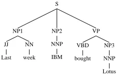
Figure 1: An example parse tree.
until the processing of its children is completed. For example, in Figure 1, when the constituent NP3 is created, it starts a nested structure of degree 2, since two levels of its ancestors (VP, S) are still processed. Its parent (VP) starts a nested structure of degree 1.
The difficulty of deeply nested structures for the human parser is well established in the psycholin-guistics literature. We review here some of the vari-ous explanations of this phenomenon; for a compre-hensive review see (Gibson, 1998).
According to the classical stack overflow theory (Chomsky and Miller, 1963) and its extension, the incomplete syntactic/thematic dependencies theory (Gibson, 1991), the human parser should track the open structures in its short term memory. When the number of these structures is too large or when the structures are nested too deeply, the short term mem-ory fails to hold them and the sentence becomes un-interpretable.
According to the perspective shifts theory (MacWhinney, 1982), processing deeply nested structures requires multiple shifts of the annotator perspective and is thus more difficult than process-ing shallow structures. The difficulty of deeply nested structured has been demonstrated for many languages (Gibson, 1998).
We thus propose the total number of nested struc-tures of degreeK in a sample (TNSK) as a measure of the cognitive efforts that its annotation requires. The higherKis, the more demanding the structure.
Sentence level resources. In the
con-stituents or nested structures) require more cognitive resources for longer periods.
Levelt (2001) suggested a layered model of the mental lexicon organization, arguing that when one hears or reads a sentence s/he activates word forms (lexemes) that in turn activate lemma information. The lemma information contains information about syntactic properties of the word (e.g., whether it is a noun or a verb) and about the possible sentence structures that can be generated given that word. The process of reading words and retrieving their lemma information is incremental and the lemma informa-tion for a given word is used until its syntactic struc-ture is completed. The information about a word in-clude all syntactic predictions, obligatory (e.g., the prediction of a noun following a determiner) and op-tional (e.g., opop-tional arguments of a verb, modifier relationships). This information might be relevant long after the constituents containing the word are closed, sometimes till the end of the sentence.
Another line of research focuses on working memory, emphasizing the activation decay princi-ple. It stresses that words and structures perceived during sentence processing are forgotten over time. As the distance between two related structures in a sentence grows, it is more demanding to reactivate one when seeing the other. Indeed, supported by a variety of observations, many of the theories of the human parser (see (Lewis et al., 2006) for a sur-vey) predict that processing items towards the end of longer sentences should be harder, since they most often have to be integrated with items further back. Thus, sentences with a large number of structures impose a special cognitive load on the annotator.
We thus propose to use the number of structures (constituents or nested structures) in a sentence as a measure of its difficulty for human annotation. The measures we use for a sample (a sentence set) are the
average number of constituents (AC) and the
aver-age number of nested structures of degreek(ANSK) per sentence in the set. Higher AC orANSK values of a set imply higher annotation requirements3.
Pschycolinguistics research makes finer
observa-3
The correlation between the number of constituents and sentence length is very strong (e.g., correlation coefficient of 0.93 in WSJ section 0). We could use the number of words, but we prefer the number of structures since the latter better reflects the arguments made in the literature.
tions about the human parser than those described here. A complete survey of that literature is beyond the scope of this paper. We consider the proposed measures a good approximation of some of the hu-man parser characteristics.
4 Parameter Based Sampling (PBS)
Our approach is to sample the unannotated pool with respect to the distribution of the model parameters in its sentences. In this paper, in order to compare to previous works, we apply our methods to the Collins generative parser (Collins, 1999). For any sentence
s and parse tree t it assigns a probability p(s, t), and finds the tree for which this probability is maxi-mized. To do that, it writesp(t, s)as a product of the probabilities of the constituents intand decomposes the latter using the chain rule. In simplified notation, it uses:
p(t, s) =YP(S1→S2. . . Sn) =YP(S1)·. . .·P(Sn|φ(S1. . . Sn))
(1)
We refer to the conditional probabilities as the model
parameters.
Cluster Based Sampling (CBS). We describe here a method for sampling subsets that leads to a parameter estimation that is similar to the parame-ter estimation we would get if annotating the whole unannotated set.
To do that, we randomly selectM sentences from the unlabelled pool N, manually annotate them, train the parser with these sentences and parse the rest of the unlabelled pool (G = N −M). Using this annotation we build a syntactic vector repre-sentation for each sentence in G. We then cluster these sentences and sample the clusters with respect to their weights to preserve the distribution of the syntactic features. The selected sentences are man-ually annotated and combined with the group ofM
sentences to train the final parser. The size of this combined sample is measured when the annotation efforts are evaluated.
features in the vector representation of each sentence inG. Thei-th coordinate is given by the equation:
X
c∈t(s)
X
i
Fi(Q(c) ==i)·L(c) (2)
Wherec are the constituents of the sentence parse
t(s), Q is a function that returns the (P, H) pair of the constituentc,Fi is a predicate that returns 1 iff it is given pair number i as an argument and 0 otherwise, and L is the number of modifying non-terminals in the constituent plus 1 (for the head), counting the number of parameters that condition on (P, H). Following equation (2), theith coordi-nate of the vector representation of a sentence inG
contains the number of parameters that will be cal-culated conditioned on theith(P, H)pair.
We use the k-means clustering algorithm, with the
L2norm as a distance metric (MacKay, 2002), to di-vide vectors into clusters. Clusters created by this algorithm contain adjacent vectors in a Euclidean space. Clusters represent sentences with similar fea-tures values. To initialize k-means, we sample the initial centers values from a uniform distribution over the data points.
We do not decide on the number of clusters in ad-vance but try to find inherent structure in the data. Several methods for estimating the ‘correct’ num-ber of clusters are known (Milligan and Cooper, 1985). We used a statistical heuristic called the elbow test. We define the ‘within cluster disper-sion’ Wk as follows. Suppose that the data is di-vided into k clusters C1. . . Ck with |Cj| points in the jth cluster. Let Dt = Pi,j∈Ctdi,j where
di,j is the squared Euclidean distance, thenWk :=
Pk
t=1 2|1Ct|Dt. Wktends to decrease monotonically
askincreases. In many cases, from somekthis de-crease flattens markedly. The heuristic is that the location of such an ‘elbow’ indicates the appropriate number of clusters. In our experiments, an obvious elbow occurred for 15 clusters.
ki sentences are randomly sampled from each cluster, ki = DP|Ci|
j|Cj|
, where D is the number
of sentences to be sampled fromG. That way we ensure that in the final sample each cluster is repre-sented according to its size.
CMM Sampling. All of the parameters in the Collins parser are conditioned on the constituent’s
head word. Since word statistics are sparse, sam-pling from clusters created according to a lexical vector representation of the sentences does not seem promising4.
Another way to create a sample from which the parser can extract robust head word statistics is to select a sample containing many examples of each word. More formally, we denote the words that oc-cur in the unlabelled pool at leastttimes by t-words, wheretis a parameter of the algorithm. We want to select a sample containing at leasttexamples of as many t-words as possible.
To select such a sample we introduce a novel op-timisation problem. Our problem is a variant of the multiset multicover (MM) problem, which we call the constrained multiset multicover (CMM) prob-lem. The setting of the MM problem is as fol-lows (Hochbaum, 1997): Given a set I of m ele-ments to be covered eachbi times, a collection of multisetsSj ⊂I,j∈J ={1, . . . , n}(a multiset is a set in which members’ multiplicity may be greater than 1), and weightswj, find a subcollection C of multisets that covers eachi∈Iat leastbitimes, and such thatPj∈Cwjis minimized.
CMM differs from MM in that in CMM the sum of the weights (representing the desired number of sentences to annotate) is bounded, while the num-ber of covered elements (representing the t-words) should be maximized. In our case, I is the set of words that occur at least t times in the unlabelled pool,bi =t,∀i∈I, the multisets are the sentences in that pool andwj = 1,∀j∈J.
Multiset multicover is NP-hard. However, there is a good greedy approximation algorithm for it. De-fine a(sj, i) = min(R(sj, i), di), where di is the difference between bi and the number of instances of itemithat are present in our current sample, and
R(sj, i)is the multiplicity of thei-th element in the multisetsj. DefineA(sj)to be the multiset contain-ing exactlya(sj, i) copies of any element iif sj is not already in the set cover and the empty set if it is. The greedy algorithm repeatedly adds a set mini-mizing wj
|A(sj)|. This algorithm provenly achieves an approximation ratio betweenln(m)andln(m) + 1. In our case all weights are 1, so the algorithm would
4
simply add the sentence that maximizesA(sj)to the set cover.
The problem in directly applying the algorithm to our case is that it does not take into account the de-sired sample size. We devised a variant of the algo-rithm where we use a binary tree to ‘push’ upwards the number of t-words in the whole batch of unan-notated sentences that occurs at least t times in the selected one. Below is a detailed description.D de-notes the desired number of items to sample.
The algorithm has two steps. First, we iter-atively sample (without replacement) D multisets (sentences) from a uniform distribution over the multisets. In each iteration we calculate for the se-lected multiset its ‘contribution’ – the number of items that cross the threshold oftoccurrences with this multiset minus the number of items that cross thetthreshold without this multiset (i.e. the contri-bution of the first multiset is the number of t-words occurring more thanttimes in it). For each multiset we build a node with a key that holds its contribu-tion, and insert these nodes in a binary tree. Inser-tion is done such that all downward paths are sorted in decreasing order of key values.
Second, we iteratively sample (from a uniform distribution, without replacement) the rest of the multisets pool. For each multiset we perform two steps. First, we prepare a node with a key as de-scribed above. We then randomly chooseZ leaves5 in the binary tree (if the number of leaves is smaller thanZall of the leaves are chosen). For each leaf we find the place of the new node in the path from the root to the leaf (paths are sorted in decreasing order of key values). We insert the new node to the high-est such place found (if the new key is not smaller than the existing paths), add its multiset to the set of selected multisets, and remove the multiset that cor-responds to the leaf of this path from the batch and the leaf itself from the binary tree. We finally choose the multisets that correspond to the highestDnodes in the tree.
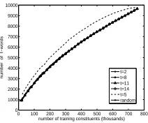
An empirical demonstration of the quality of ap-proximation that the algorithm provides is given in Figure 2. We ran our algorithm with the threshold parameter set to t ∈ [2,14] and counted the
num-5
We triedZ values from 10 to 100 in steps of 10 and ob-served very similar results. We report results forZ= 100.
0 100 200 300 400 500 600 700 800 0
1000 2000 3000 4000 5000 6000 7000 8000 9000 10000
number of training constituents (thousands)
number of t−words
[image:6.612.374.480.54.142.2]t=2 t=8 t=11 t=14 t=5 random
Figure 2: Number of t-words for t = 5 in samples selected
byCMM runs with different values of the threshold
pa-rameter t and in a randomly selected sample. CMMwith
t = 5 is significantly higher. All the lines except for the line for t = 5 are unified. For clarity, we do not show all t
values: their curves are also similar to thet6= 5lines.
Method 86% 86.5% 87% 87.5% 88%
TE 16.9% 27.1% 26.9% 14.8% 15.8%
(152K) (183K) (258K) (414K) (563 K)
CBS 19.6% 16.8% 19% 21.1% 9%
(147K) (210K) (286K) (382K) (610K)
[image:6.612.334.519.249.300.2]CMM 9% 10.4% 8.9% 10.3% 14% (167K) (226K) (312K) (433K) (574K)
Table 1: Reduction in annotation cost inTCterms
com-pared to the random baseline for tree entropy (TE),
syn-tactic clustering (CBS) andCMM. The compared samples
are the smallest samples selected by each of the methods that achieve certain f-score levels. Reduction is
calcu-lated by:100−100×(T Cmethod/T Crandom).
ber of words occurring at least 5 times in the se-lected sample. We followed the same experimen-tal protocol as in Section 5. The graph shows that the number of words occurring at least 5 times in a sample selected by our algorithm whent= 5is sig-nificantly higher (by about a 1000) than the number of such words in a randomly selected sample and in samples selected by our algorithm with othert pa-rameter values. We got the same pattern of results when counting words occurring at leastttimes for the other values of thetparameter – only the run of the algorithm with the correspondingtvalue created a sample with significantly higher number of words not below threshold. The other runs and random se-lection resulted in samples containing significantly lower number of words not below threshold.
86% 87% 88%
Method TNSK TNSK ANSK ANSK TNSK TNSK ANSK ANSK TNSK TNSK ANSK ANSK (1-6) (7-22) (1-6) (7-22) (1-6) (7-22) (1-6) (7-22) (1-6) (7-22) (1-6) (7-22)
TE 34.9% 3.6% - 8.9% - 61.3% 42.2% 14.4% - 9.9% - 62.7% 25% 8.1% - 6.3% - 30%
[image:7.612.115.500.55.101.2]CBS 21.3% 18.6% - 0.5% - 3.5% 19.6% 24.2% - 0.3% - 1.8% 8.9% 8.6 % 0% - 0.3% CMM 10.18% 8.87% -0.82% -3.39% 11% 16.22% -0.34% -1.8% 14.65% 14.11% -0.02% - 0.08%
Table 2: Annotation cost reduction inTNSKandANSKcompared to the random baseline for tree entropy (TE), syntactic
clustering (CBS) andCMM. The compared samples are the smallest selected by each of the methods that achieve certain
f-score levels. Each column represents the reduction in total or average number of structures of degree 1–6 or 7–22.
Reduction for each measure is calculated by:100−100×(measuremethod/measurerandom). Negative reduction
is an addition. Samples with a higher reduction in a certain measure are better in terms of that measure.
0 5 10 15 20 25
−1 0 1 2 3
x 104
K
TNSK (K)
CMM(t=8) − TE CBS − TE 0 line
0 5 10 15 20 25 1
1.1 1.2 1.3 1.4 1.5 1.6 1.7
K
ANSK method/ANSK random
TE CMM,t=8 CBS
86 86.5 87 87.5 88 18
20 22 24 26 28
F score
Average number of constituents
TE CMM, t = 8 CBS
0 1 2 3 3.5
x 104 1
1.25 1.5
Number of sentences
AC method/AC random
TE CMM, t=8 CBS
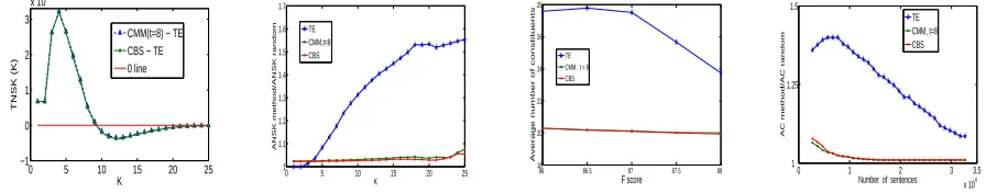
Figure 3: Left to right: First: The difference between the number of nested structures of degreeKofCMMandTEand
ofCBSandTE. The curves are unified. The0curve is given for reference. Samples selected byCMMandCBShave
more nested structures of degrees 1–6 and less nested structures of degrees 7–22. Results are presented for the smallest samples required for achieving f-score of 88. Similar patterns are observed for other f-score values. Second: Average
number of nested structures of degreeKas a function ofKfor the smallest sample required for achieving f-score of
88. Results for each of the methods are normalized by the average number of nested structures of degreeKin the
smallest randomly selected sample required for achieving f-score of 88. The sentences inCMMandCBSsamples are
not more complex than sentences in a randomly selected sample. InTEsamples sentences are more complex. Third:
Average number of constituents (AC) for the smallest sample of each of the methods that is required for achieving a
given f-score.CMMandCBSsamples contain sentences with a smaller number of constituents. Fourth: ACvalues for
the samples created by the methods (normalized byACvalues of a randomly selected sample). The sentences inTE
samples, but not inCMMandCBSsamples, are more complex than sentences in a randomly selected sample.
5 Results
Experimental setup. We used Bikel’s
reimplemen-tation of Collins’ parsing model 2 (Bikel, 2004). Sections 02-21 and 23 of the WSJ were stripped from their annotation. Sections 2-21 (39832 sen-tences, about 800K constituents) were used for train-ing, Section 23 (2416 sentences) for testing. No development set was used. We used the gold stan-dard POS tags in two cases: in the test section (23) in all experiments, and in Sections 02-21 in the CBS method when these sections are to be parsed in the process of vector creation. In active learn-ing methods the unlabelled pool is parsed in each iteration and thus should be tagged with POS tags. Hwa (2004) (to whom we compare our results) used the gold standard POS tags for the same sections in her work6. We implemented a random baseline
6Personal communication with Hwa. Collins’ parser uses an
where sentences are uniformly selected from the un-labelled pool for annotation. For reliability we re-peated each experiment with the algorithms and the random baseline 10 times, each time with different random selections (Msentences for creating syntac-tic tagging and k-means initialization for CBS, sen-tence order inCMM), and averaged the results.
Each experiment contained 38 runs. In each run a different desired sample size was selected, from 1700 onwards, in steps of 1000. Parsing perfor-mance is measured in terms of f-score
Results. We compare the performance of our CBS andCMMalgorithms to theTE method (Hwa, 2004)7, which is the only sample selection work
ad-input POS tag only if it cannot tag its word using the statistics learned from the training set.
7Hwa has kindly sent us the samples selected by her
TE. We evaluated these samples withTCand the new measures. TheTC
[image:7.612.79.532.183.271.2]dressing our experimental setup. Unless otherwise stated, we report the reduction in annotation cost:
100−100×(measuremethod/measurerandom).
CMMresults are very similar fort∈ {2,3, . . . ,14}, and presented fort= 8.
Table 1 presents reduction in annotation cost in TC terms. CBS achieves greater reduction for f = 86,87.5, TEforf = 86.5,87,88. Forf = 88, TE andCMMperformance are almost similar. Examin-ing the f-score vs. TC sample size over the whole constituents range (not shown due to space con-straints) reveals that CBS, CMMandTE outperform random selection over the whole range. CBS and TEperformance are quite similar withTEbeing bet-ter in the ranges of 170–300K and 520–650K con-stituents (42% of the 620K concon-stituents compared) andCBSbeing better in the ranges of 130–170K and 300–520K constituents (44% of the range). CMM performance is worse than CBS andTE until 540K constituents. From 650K constituents on, where the parser achieves its best performance, the perfor-mance ofCMMandTEmethods are similar, outper-formingCBS.
Table 2 shows the annotation cost reduction in ANSK and TNSK terms. TE achieves remarkable reduction in the total number of relatively shallow structures (TNSK K = 1–6). Our methods, in con-trast, achieve remarkable reduction in the number of deep structures (TNSK K= 7–22)8. This is true for all f-score values. Moreover, the average number of nested structures per sentence, for every degree K
(ANSKfor everyK) inTEsentences is much higher than in sentences of a randomly selected sample. In samples selected by our methods, theANSK values are very close to the ANSK values of randomly se-lected samples. Thus, sentences in TEsamples are much more complex than inCBSandCMMsamples.
The two leftmost graphs in Figure 3 demonstrate (for the minimal samples required for f-score of 88) that these reductions hold for eachK value (ANSK) and for eachK ∈ [7,22](TNSK) not just on the
av-of 88 is different from the number reported in (Hwa, 2004). We compare ourTCresults with theTCresult in the sample sent us by Hwa.
8
We present results where the border between shallow and deep structures is set to beKborder = 6. For everyKborder ∈
{7,8, . . . ,22}TNSKreductions withCBSandCMMare much more impressive than withTE for structures whose degree is
K∈[Kborder,22].
erage over theseK values. We observed similar re-sults for other f-score values.
The two rightmost graphs of Figure 3 demon-strates AC results. The left of them shows that for every f-score value, theACmeasure of the minimal TEsample required to achieve that f-score is higher than theAC value of PBS samples (which are very similar to the ACvalues of randomly selected sam-ples). The right graph demonstrates that for every sample size, the AC value of TE samples is higher than that of PBS samples.
All AL based previous work (includingTE) is it-erative. In each iteration thousands of sentences are parsed, while PBS algorithms perform a single iteration. Consequently, PBS computational com-plexity is dramatically lower. Empirically, using a Pentium 4 2.4GHz machine,CMMrequires about an hour andCBSabout 16.5 hours, while theTEparsing steps alone take 662 hours (27.58 days).
6 Discussion and Future Work
We introduced novel evaluation measures: AC, TNSK and ANSK for the task of sample selection for statistical parsers. Based on the psycholinguis-tic literature we argue that these measures reflect as-pects of the cognitive efforts of the human annota-tor that are not reflected by the traditionalTC mea-sure. We introduced the parameter based sample se-lection (PBS) approach and itsCMMandCBS algo-rithms that do not deliberately select difficult sen-tences. Therefore, our intuition was that they should select a sample that leads to an accurate parameter estimation but does not contain a high number of complex structures. We demonstrated thatCMMand CBSachieve results that are similar to the state of the art TEmethod in TCterms and outperform it when the cognitively driven measures are considered.
The measures we suggest do not provide a full and accurate description of human annotator efforts. In future work we intend to extend and refine our measures and to revise our algorithms accordingly.
References
Steven Abney and Mark Johnson, 1991. Memory re-quirements and local ambiguities of parsing strategies.
Psycholinguistic Research, 20(3):233–250.
Daniel M. Biken, 2004. Intricacies of Collins’ parsing model. Computational Linguistics, 30(4):479–511. Jason Baldridge and Miles Osborne, 2004. Active
learn-ing and the total cost of annotation. EMNLP ’04. Markus Becker and Miles Osborne, 2005. A two-stage
method for active learning of statistical grammars.
IJ-CAI 05.
Markus Becker, 2008. Active learning – an explicit treat-ment of unreliable parameters. Ph.D. thesis, The Uni-versity of Edinburgh.
Noam Chomsky and George A. Miller, 1963.
Fini-tary models of language users. In R. Duncan Luce, Robert R. Bush, and Eugene Galanter, editors,
Hand-book of Mathematical Psychology, volume II. John
Wiley, New York, 419–491.
David Cohn, Les Atlas and Richard E. Ladner, 1994. Im-proving generalization with active learning. Machine
Learning, 15(2):201–221.
Michael Collins, 1999. Head-driven statistical models
for natural language parsing. Ph.D. thesis, University
of Pennsylvania.
Edward Gibson, 1991. A computational theory of
hu-man linguistic processing: memory limitations and processing breakdowns. Ph.D. thesis, Carnegie
Mel-lon University, Pittsburg, PA.
Edward Gibson, 1998. Linguistic complexity: locality of syntactic dependencies. Cognition, 68:1–76. Dorit Hochbaum (ed), 1997. Approximation algorithms
for NP-hard problems. PWS Publishing, Boston.
Rebecca Hwa, 2004. Sample selection for statistical
parsing. Computational Linguistics, 30(3):253–276. Cody Kwok, Oren Etzioni, Daniel S. Weld, 2001.
Scal-ing question answerScal-ing to the Web. WWW ’01. Matthew Lease and Eugene Charniak, 2005. Parsing
biomedical literature. IJCNLP ’05.
Willem J.M. Levelt, 2001. Spoken word production: A theory of lexical access. PNAS, 98(23):13464–13471. Richard L. Lewis, Shravan Vasishth and Julie Van Dyke,
2006. Computational principles of working memory in sentence comprehension. Trends in Cognitive
Sci-ence, October:447-454.
David MacKay, 2002. Information theory, inference and
learning algorithms. Cambridge University Press.
Brian MacWhinney, 1982. The competition model. In B. MacWhinney, editor, Mechanisms of language
ac-quisition. Hillsdale, NJ: Lawrence Erlbaum, 249–308.
Daniel Marcu, Wei Wang, Abdessamabad Echihabi, and
Kevin Knight, 2006. SPMT: Statistical machine
translation with syntactified target language phrases.
EMNLP ’06.
P. Melville, M. Saar-Tsechansky, F. Provost and R.J. Mooney, 2005. An expected utility approach to ac-tive feature-value acquisition. 5th IEEE Intl. Conf. on
Data Mining ’05.
Mitchell P. Marcus, Beatrice Santorini, and Mary Ann Marcinkiewicz, 1994. Building a large annotated cor-pus of English: The Penn treebank. Computational
Linguistics, 19(2):313–330.
G.W. Milligan and M.C Cooper, 1985. An examination of procedures for determining the number of clusters in a data set. Psychometrika, 58(2):159–157.
Grace Ngai and David Yarowski, 2000. Rule writing or annotation: cost–efficient resource usage for base noun phrase chunking. ACL ’00.
Roi Reichart, Katrin Tomanek, Udo Hahn and Ari Rap-poport, 2008. Multi-task active learning for linguistic annotations. ACL ’08.
Brian Roark, Margaret Mitchell and Kristy Hollingshead,
2007. Syntactic complexity measures for detecting
mild cognitive impairment. BioNLP workshop, ACL
’07.
Min Tang, Xiaoqiang Luo, and Salim Roukos, 2002. Ac-tive learning for statistical natural language parsing.
ACL ’02.
Katrin Tomanek, Joachim Wermtre, and Udo Hahn, 2007. An approach to text corpus construction which cuts annotation costs and maintains reusability of an-notated data. EMNLP ’07.
Kristina Toutanova, Aria Haghighi, and Christopher D. Manning, 2005. Joint learning improves semantic role labeling. ACL ’05.