GraphBTM: Graph Enhanced Autoencoded Variational Inference
for Biterm Topic Model
Qile Zhu, Zheng Feng, Xiaolin Li Large-scale Intelligent Systems Laboratory
NSF Center for Big Learning University of Florida
{valder, fengzheng}@ufl.edu, [email protected]
Abstract
Discovering the latent topics within texts has been a fundamental task for many applica-tions. However, conventional topic models suffer different problems in different settings. The Latent Dirichlet Allocation (LDA) may not work well for short texts due to the data sparsity (i.e., the sparse word co-occurrence patterns in short documents). The Biterm Topic Model (BTM) learns topics by mod-eling the word-pairs named biterms in the whole corpus. This assumption is very strong when documents are long with rich topic in-formation and do not exhibit the transitivity of biterms. In this paper, we propose a novel way called GraphBTM to represent biterms as graphs and design Graph Convolutional Net-works (GCNs) with residual connections to extract transitive features from biterms. To overcome the data sparsity of LDA and the strong assumption of BTM, we sample a fixed number of documents to form a mini-corpus as a training instance. We also propose a dataset calledAll N ews extracted from (Thompson,
2017), in which documents are much longer than 20 Newsgroups. We present an amortized variational inference method for GraphBTM. Our method generates more coherent topics compared with previous approaches. Exper-iments show that the sampling strategy im-proves performance by a large margin.
1 Introduction
Topic model (Blei et al.,2003) is one of the most popular approaches to learn hidden representa-tions of text. The broad applications of topic model range from recommender systems (Wang and Blei, 2011), computer vision (Fei-Fei and Perona, 2005), to bioinformatics (Rogers et al.,
2005). Conventional topic models learning ap-proaches are based on Gibbs Sampling ( Grif-fiths and Steyvers, 2004) or Variational Expecta-tion MaximizaExpecta-tion (VEM) algorithm (Blei et al.,
2003). Both Gibbs Sampling and VEM are not directly applicable to new variations of the topic model. Specifically, the inference algorithm re-quires re-deriving for any minor changes to the model.
Recently, a neural network based topic model inference approach, the Autoencoded Variational Inference for Topic Model (AVITM), was pro-posed by (Srivastava and Sutton,2017). This ap-proach uses an inference network to directly map a document to its posterior distribution without any variational update steps. The proposed in-ference network is based on the Autoencoding Variational Bayes (AEVB) (Kingma and Welling,
2013), a stochastic variational inference algorithm over neural networks. Compared with the sam-pling based approaches, AVITM can scale to large datasets. Although it improves the model’s robust-ness and reduces the computational cost, it still suffers from the data sparsity in short texts.
Biterm Topic Model (BTM) proposed by (Cheng et al., 2014) and (Yan et al., 2013) ad-dresses the shortcoming of data sparsity for eling the corpus of short texts. It explicitly mod-els the patterns on top of word co-occurrence fea-ture (Biterm, the unordered word-pair occurs in texts) from the corpus. It holds one topic distri-bution for the whole corpus rather than one doc-ument. BTM, therefore, is suitable for modeling short documents like tweets, and online QA texts. It also achieves better results than LDA in specific scenarios of the normal texts (Yan et al., 2013). However, using one topic distribution for all docu-ments limits the model’s expressiveness when the documents contain diverse topics.
whole corpus, we extract biterms inside a fixed-length text window for every document and sam-ple n documents to form an instance each time. As a result, we enhance the input feature with biterms that capture more word co-occurrence pat-terns than BOW and also avoid the insufficient corpus-wised topic representation in BTM. An-other advantage of biterms is the transitivity. For example, we have two biterms(A, B)and(A, C). It is natural to think thatBandCmay share some similarities. This transitivity is similar to the graph structure data. So we model the biterms in a graph where the words are taken as nodes and the counts of biterms are the weight of edges. We extract the information from biterms explicitly by the graph convolutional network (Kipf and Welling,2016).
In this paper, we propose a novel Graph-based inference network for the biterm topic model (GraphBTM). To the best of our knowledge, GraphBTM is the first AEVB inference approach for the biterm topic model with graph enhanced feature. Our model also strikes a good balance be-tween LDA and BTM, leverages both advantages, and achieves better topics coherence scores than AVITM in two datasets. The main contributions of our work include:
• We are the first to apply the neural network based inference approach for the Biterm Topic Model, and achieve better results in
topic coherence score than previous AEVB based inference method (AVITM) and online Variational Inference LDA.
• We propose a data argumentation method to enhance the input feature with word corre-lation from biterms in normal text and over-come the shortcoming of the data sparsity in LDA and the insufficient corpus-wise topic representation in BTM.
• We model the biterms as an undirected graph and adopt a novel graph convolutional net-work to encode word co-relationship in our inference network.
• We introduce a new dataset All N ews
dataset containing 20,000 documents ex-tracted from 15 news publishers (Thompson,
2017) for topic modeling. TThe documents are much longer compared with the 20 News-groups.
2 Background
2.1 Biterm Topic Model
BTM (Cheng et al.,2014) is proposed to solve the data sparsity problem in the scenario of short texts. Instead of modeling a single document, BTM con-siders the whole corpus as a mixture of topics. BTM collects all unordered word-pairs (biterms) from each short text or a fixed-length text window of normal texts. The generative progress of BTM can be described as follows, where α and β are two parameters of Dirichlet priors.
1. For each topic z
(a) draw a topic-specific word distribution
φz ∼Dir(β)
2. Draw a topic distributionθ∼Dir(α)for the whole corpus
3. For each biterm b in the biterm set
(a) draw a topic assignmentz∼M ulti(θ)
(b) draw two words:wi, wj ∼M ulti(φz)
With the procedure above, the joint probability of a bitermb= (wi, wj)can be written as:
P(b) =X z
P(z)P(wi|z)P(wj|z) (1)
=X z
θzφi|zφj|z (2)
So the likelihood of the whole corpusBis:
P(B|α, β) =Y i,j
X z
θzφi|zφj|z (3)
2.2 Laplace Approximation of Dirichlet
Both LDA and BTM use the Dirichlet prior over the topic and word proportions. Wallach et al.
(2009) showed that the Dirichlet prior is important to producing interpretable topics. However, it is hard to apply the Dirichlet prior to AEVB directly. AEVB uses the reparameterization trick (RT) to obtain a differentiable Monte Carlo estimator for the variational lower bound (details can be found in next section), and it is difficult to propose an effective RT for the Dirichlet prior.
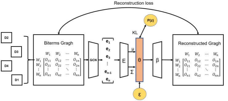
Figure 1: The overall structure of our proposed model GraphBTM. In this example, we sample 4 documents at a time and embed the aggregated biterm graph by GCNs. The graph embedding is sent to inference network E to produce the parameters for our variational distribution. We then use RT to generate the Monte Carlo samples. At last, we use the decoder networkβto get the word probabilities and reconstruct the aggregated graph.
2012). MacKay (1998) gives the Dirichlet prob-ability density function in the softmax basis over the variablex:
P(π|α) = Γ( PK
k(αk)) QK
k Γ(αk) Y
k παk
k g(1
Tx) (4)
whereπ =σ(x)(softmax) andg(1Tx)is an arbi-trary density for integrability.Hennig et al.(2012) argued that the Eq. 4 could be approximately in-dependent for largeK (number of topics). So the covariance matrix of the Dirichlet prior becomes a diagonal matrix for largeK. By this way, we can approximate the Dirichlet distribution with a multivariate normal with meanµkand covariance
matrixΣkk:
µk=logαk− 1 K
K X
i
logαi (5)
Σkk= 1 αk(1−
2 K) +
1 K2
K X
i 1
αi (6)
with this approximation in hand, we can easily ap-ply RT by sampling from ∼ N(0, I) and com-pute probabilityπk=σ(µk+ Σ1kk/2).
3 Graph Biterm Topic Model
Before getting into details of GraphBTM, we give an overall structure of GraphBTM, as shown in Fig.1. We extract the biterms from a mini-corpus (aggregated sampled documents) and embed the whole biterm graph into a fixed length vector with the dimension of vocabulary size. Then we use
this graph embedding as the input of our inference network and get the topic proportion. At last, we use the decoder network to get the word probabil-ities and reconstruct the biterm graph.
3.1 Model Biterms as Graphs
Commonly used input feature of topic models is bag-of-words (BOW) which implicitly capture the word co-occurrence patterns. BTM models the word co-occurrence explicitly by directly counting the word-pairs in a text window. However, using one-hot encoding for biterms may lose the transi-tive co-relations. We model collected biterms as a graph G = (V,E), where V (words as nodes and|V|is the vocabulary size) and E (counts of corresponding biterms in the sample) are sets of nodes and edges, respectively. In this way, the ad-jacency matrixA(A∈RV×V) denotes the counts of biterms in the sample. We also leverage the ma-trixA as the node feature matrix (Ai is the node
feature for the wordwi).
We use GCNs proposed by (Kipf and Welling,
2016), which is a framework used for learning the graph structure data. Gilmer et al. (2017) presented a comprehensive overview. Consider an undirected graph G = (V,E) and a matrix
X ∈ Rn×m in where each row is a node feature xv ∈ Rm (v ∈ V). One layer GCN encodes
in-formation of a node with its immediate neighbors, defined as
hl+1 =f
˜
D−0.5A˜D˜−0.5(hlWl+b)
(7)
is the adjacency matrix of the graph with self-connections, IN is the identity matrix, D˜ is the degree matrix ofA˜, Wl is a trainable weight ma-trix in the layer and b is the bias. f denotes a non-linear activation function, such as ReLU. By stacking GCN layers, we can incorporate higher order neighborhoods. To represent the whole graph, we reduce the dimension of each node to one by using GCNs and concatenate them as the final representation of the biterm graph.
From another point of view, we can treat GCNs as a Laplacian smoothing. Repeatedly applying Laplacian smoothing may mix the features of ver-tices and make them indistinguishable (Li et al.,
2018). On the other hand, the transitivity of words may not be meaningful when the number of hops (layers) of GCN increases. We solve this prob-lem by adding shortcut connections between dif-ferent layers inspired by Residual Networks (He et al.,2016). What’s more, a recent study showed that adding the residual connection can help con-vergence (Li and Yuan,2017).
3.2 AEVB for Biterm Graphs
Eq. 3gives us the likelihood of the whole corpus based onM ulti(φz). Here we rewrite the Eq. 3
with latent variables as
p(B|α, β) = Z
θ
Y
(i,j)
k X z=1
πiπjp(zn|θ)
p(θ|α)dθ
(8)
whereπi = p(wi|zn, β). The inference of
poste-riorp(θ, z|B, α, β)over the hidden variablesθand
zis intractable (Dickey,1983). Many methods are proposed to solve this inference problem includ-ing Gibbs Samplinclud-ing (Griffiths and Steyvers,2004) and variational inference methods. Gibbs Sam-pling based approaches are computationally inef-ficient and varitional inference methods like mean field (Blei et al., 2003) scarify the topic quality for computational efficiency. Moreover, the ma-jor problem of these approximate inference algo-rithms is the inflexibility. Slight changes in model assumption may require designing a new infer-ence algorithm. To alleviate this problem, we de-sign an amortized approximate inference method similar to AVITM (Srivastava and Sutton,2017). It is more flexible compared with other approxi-mate inference methods and can be applied to any biterm graphs.
In Eq. 8, there are two latent variables θ and
z, we introduce two free variational parametersγ
overθandφoverz. Our goal is to approximate the true posteriorp(θ, z|B, α, β) with variational distributionq(θ, z|γ, φ) =qγ(θ)Q
kqφ(zk). Then
we can transfer the inference problem as an opti-mization problem (Blei et al.,2003), which is to maximize
L(γ, φ|α, β) =logp(B|α, β) (9) −DKL[q(θ, z|γ, φ)||p(θ, z|B, α, β)]
Lis a lower bound to the marginal log likelihood (ELBO). Following AEVB (Kingma and Welling,
2013), we rewrite the ELBO as
L(γ, φ|α, β) =−DKL+R (10)
whereR = Eq[logp(B|z, θ, α, β)]. This form is
intuitive. The first term is the KL divergence be-tweent the variational distribution and the prior on the latent variables, and the second term ensures that the latent variables are good at explaining and reconstructing the input data.
We use a neural network named inf erence networkto compute the variational parameters. It takes the embedding of the biterm graph (sec.3.1) as the input and outputs the parameters of the vari-ational distribution. So the inference network can be defined as(µb,Σb) =f(b, γ), whereµbandΣb
are vectors of lengthk(topic numbers) andγ are the network parameters. In our setting, we use the logistic normal distribution which is an approxi-mation of the Dirichlet prior to the variational dis-tribution. We can choose the corresponding vari-ational distributionqγ(θ) =LN(θ|µb, diag(Σb)), where diag(·) converts a column vector to a di-agonal matrix. One important advantage of using AEVB is that we couple the variational parame-ters for different inputs, unlike mean field varia-tional inference, because they are computed from the same network.
Although the reparameterization trick helps us deal with θ, it is hard to deal with the discrete variable z. Fortunately, we can collapse the dis-crete variables z and only infer θ with collapsed inference method (Kurihara et al.) as
p(B|α, β) = Z
θ
Y
(i,j)
πiπj
p(θ|α)dθ (11)
where πi = p(wi|β, θ), which is the probability
of one word in the biterm. Now we only need to sampling fromθ.
We can now get our final variational objective function as (to minimize the negative ELBO)
L=DKL−E[XGb◦log(PTP)] (12)
where Gb is the input biterm graph, P = σ(β)σ(µ + Σ1/2) is probabilities for all the words based on the input graph and◦denotes the element-wise production. The KL divergence be-tween two logistic normal distritbutions are
DKL=1 2{tr(Σ
−1
1 Σ0) + (µ1−µ0)TΣ−11(µ1−µ0)
−K+log|Σ1|
|Σ0|
} (13)
3.3 Sample Mini-corpus
To alleviate the data sparsity problem of LDA (Zhu and Xing, 2012; Lin et al., 2014), BTM learns topics from the aggregated patterns in the whole corpus. In our observation, this assumption is too strong for normal texts. Other than BTM, some approaches in the literature addressed this problem by aggregating documents into a mini-corpus before training the topic model. For ex-ample, in tweets analysis, Weng et al.(2010) ag-gregated the tweets from one user into a docu-ment. Hong and Davison (2010) combined the tweets containing the same word. Inspired by these strategies, we make the same assumption for normal text. We first extract all the biterms in each document and randomly selectndocuments in the dataset as a corpus. The biterms of the mini-corpus simply merge all the biterms from the n
documents. Experiments show that a proper sam-pling number achieves the best performance.
3.4 Unnormalize theβ
The topic-word distribution β is a mixture of multinomials. One drawback of this formula-tion is that it cannot predict something that is
sharper than the distributions being mixed ( Hin-ton and Salakhutdinov,2009). This problem may result in some poor quality topics. Previous re-search (Srivastava and Sutton, 2017) shows that unnormalizing the parameters β and changing the conditional distribution of wn as wn|β, θ ∼
M ultinomial(1, σ(βθ))can solve this problem. With the unnormalized β, we can model it as a decoder network whose weight matrix M = (m1, . . . , mK) denotes the weight for all words
underK topics. Applying softmax to rowmiwill give us the probabilities under topici.
4 Experiments
4.1 Datasets and Settings
We demonstrate our model on two datasets: 20 Newsgroups andAll N ews. For All News, we use the data from kaggle collection (Thompson,2017)
1, which collects documents from 15 main news
publishers between 2016 and July 2017. Among these, we randomly select 20,000 documents. In our preprocessing of the texts, we follow the steps of tokenization, filtering out stop words, and non-UTF-8 characters in (Srivastava and Sutton,2017). From the statistics summarized in Table1. We can know that the 20 Newsgroups dataset is relatively sparse and the All News has rich information. The ratio of text lengths less or equal to 30 of the 20 Newsgroups dataset is 28%, which only 2% in the All News dataset. The average size differs a lot between these two datasets: 302 for the All News and 88 for the 20 Newsgroups.
For the generation of the matrixWg, the
selec-tion of the window size of words is critical, a small size of window leads to very sparseWg. Here, we choose an experience value 30 for the window size follows the (Yan et al.,2013). For the logistic nor-mal approximation, we use the Dirichlet distribu-tion with parameter α as 0.02. Our GraphBTM approach, including the GCN layers and the in-ference network are implemented with Pytorch-v0.4.0 (Paszke et al.). Parameters in our imple-mented model are optimized by the stochastic op-timizer Adadelta (Zeiler,2012) with learning rate 1. To embed the biterm graph, we use a 3-layer GCNs with size 1995-100, 100-100 and 100-1 for 20 Newsgroups and 5000-1000, 1000-100, 100-1 for ALL News. We use theedge dropoutin GCN: when computinghl, we ignore each node with a probability of 0.6. We use batch normalization
Datasets Training instances Ratio of<=30 Avg size Vocabulary Avg Biterms #
20 News 11,259 28% 88 1995 1249
All News 20,000 2% 302 5000 5535
Table 1: Datasets statistics.
Dataset # topics GraphBTM AVITM LDA Online VI
20 News 50 0.28 0.25 0.10
100 0.26 0.23 0.08
All news 50 0.27 0.24 0.14
[image:6.595.81.282.253.434.2]100 0.26 0.23 0.13
Table 2: Average topic coherence.
Datasets(# Topics) # Samples Score
20 News (k=50)
1 0.24
3 0.28
10 0.25
20 News (k=100)
1 0.21
3 0.26
10 0.25
All news (k=50)
1 0.27
3 0.22
5 0.20
All news (k=100)
1 0.26
3 0.20
5 0.17
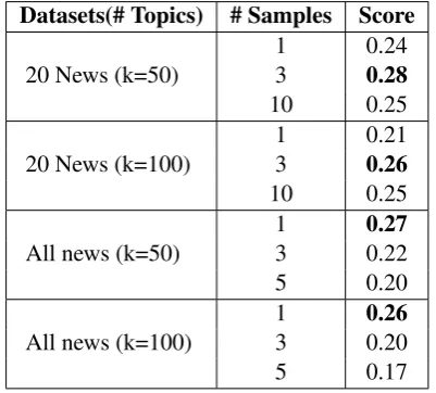
Table 3: Results for different sampling numbers in different setting for the two datasets. Score denotes the topic coherence score.
(Ioffe and Szegedy,2015) ininf erence network
with batch size 100 as same in (Srivastava and Sut-ton,2017). We run each model 10 times and take the average results. Code is available athttps: //github.com/valdersoul/GraphBTM.
The perplexity has been used in the past works to measure the quality of the generated topics. However, the perplexity is not shown to be a good evaluation metric for the topics (Newman et al.,
2010). What’s more, our method models a mini-corpus instead of a real one and infer the top-ics through the pattern of biterms, so the perplex-ity is not suitable to measure the performance of our approach. To get a more objective measure-ment of the topics, we adopt ”topic coherence” as our metric, proposed by (Mimno et al., 2011) to evaluate the quality of the topics. For a vec-torV(z) = (vz1, ..., vzT) as the topT words of the topicz, which ordered by the probabilityp(w|z),
the topic coherence is defined as:
C(z;V(z)) = T X
t=2
t X l=1
logD(v
(z)
m , v(lz)) + 1
D(vl(z)) .
(14)
whereD(v) is the number of the documents that word v occurred, and D(v, v0) is the number of the documents that both the words v and v0 oc-curred. The assumption of the topic coherence is the words with high frequency in a topic tend to appear in the same document. This measurement has been demonstrated to be highly consistent with the human evaluated quality of the topics.
4.2 Results and Discussions
Comparison with other approaches. We com-pare our GraphBTM approach with the AVITM (Srivastava and Sutton,2017) and the LDA model (Blei et al., 2003). For AVITM, we use their results for 20 Newsgroups directly and run the model using the provided code2. We use the on-line variational inference for LDA (Hoffman et al.,
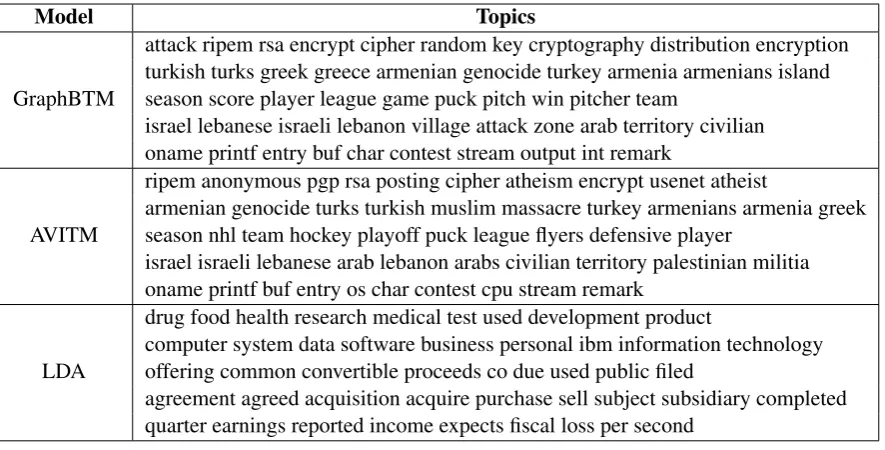
2010) implementation by gensim library (Reh˚uˇrekˇ and Sojka, 2010) as our LDA baseline. For both GraphBTM and AVITM, we run 200 iterations. Table 2 shows the average topic coherence for three models on the two datasets. The online VI LDA works worst in the three models and we find that on both datasets, the GraphBTM consis-tently outperforms other two models. We can ver-ify the quality of the learned topics by displaying the topic examples in Table 4. The topics from GraphBTM are more coherent than the topics from both AVITM and LDA model.
2https://github.com/akashgit/
Effect of the mini-corpus. To study the ef-fect of our sampling strategy which has been dis-cussed in section 3.3. Table 3 shows the perfor-mance of our model with different sample size for a mini-corpus. For the 20 Newsgroups dataset, the best performance is achieved when the sam-ple size is 3. When we do not use our samsam-ple strategy (mini-corpus is 1), the performance drops by a large margin. From Table1, we see that the average size of documents size in 20 Newsgroups is relatively short (88 compared with 302 in All News). Therefore, the 20 Newsgroups dataset may suffer from the sparsity problem. The experiment shows that our sampling strategy can help to over-come this problem. When sample size increases, the performance drops again. The biterm graph with large sample size may bring the same prob-lem of the original BTM (insufficient topic repre-sentation). Compared to 20 Newsgroups dataset, documents in the All News dataset is longer and carried more topic information, so the best perfor-mance is achieved without sampling. We find that when the sample size is larger than an optimized value, the topic coherence starts to drop.
Effect of modeling biterms as graphs.To ver-ify the effect of the graph modeling of biterms. We also do experiments on AVITM with the same sampling strategy. We use the sampling size 3 which achieves the best performance by GraphBTM in 20 Newsgroups to train AVITM model. The performance does not change a lot, with an average score of 0.25 which is the same as the score without sampling. It is not surprising to us because AVITM models the topic directly on the individual document with BOW feature. The BOW feature captures the word co-occurrence im-plicitly. So aggregating documents in AVITM can not enhance the input feature. However, our model uses GCN to capture the transitivity of biterms and can benefit from the sampling strategy a lot.
Residual connection. We add the residual con-nection between the first and second layer of GCN. On the other hand, it can also help convergence by adding residual connection (Li and Yuan, 2017). The residual can also help the network capture hierarchical information of the biterms. We re-move the residual connection with the same set-ting which achieves the best performance in these two datasets and results in a 0.1 drop in perfor-mance.
5 Related Work
In this section, we briefly summarize the related work of the topic model into two categories: nor-mal texts and short texts.
5.1 Normal Texts
The effort of uncovering the latent semantic repre-sentation of documents can be dated from the La-tent Semantic Analysis (LSA) (Deerwester et al.,
1990), which used the singular value decomposi-tion of the document matrix to get the word pat-terns. The probabilistic latent semantic analy-sis (PLSA) (Hofmann, 1999) improved the LSA model by adding a probabilistic model based on a mixture decomposition. It assumed that a docu-ment could be presented as a mixture of topics and a topic is a distribution over words. LDA added the Dirichlet priors on topic and word distributions and proposed a complete generative model.
With the rising of deep learning (LeCun et al.,
2015), researchers achieve significant improve-ment in many areas including image classifica-tion (He et al., 2016), speech recognition ( Hin-ton et al.,2012) and named entity recognition (Ma and Hovy, 2016; Zhu et al., 2018). Many at-tempts have been made for topic models based on neural networks (Hinton and Salakhutdinov,
2009;Cao et al., 2015;Miao et al.,2016; Srivas-tava and Sutton, 2017). Cao et al. (2015) em-bedded multinomial relationships between docu-ments, topics, and words in differentiable func-tions. However, they lost the stochasticity and Bayesian inference of prior functions. Miao et al.
Model Topics
GraphBTM
attack ripem rsa encrypt cipher random key cryptography distribution encryption turkish turks greek greece armenian genocide turkey armenia armenians island season score player league game puck pitch win pitcher team
israel lebanese israeli lebanon village attack zone arab territory civilian oname printf entry buf char contest stream output int remark
AVITM
ripem anonymous pgp rsa posting cipher atheism encrypt usenet atheist
armenian genocide turks turkish muslim massacre turkey armenians armenia greek season nhl team hockey playoff puck league flyers defensive player
israel israeli lebanese arab lebanon arabs civilian territory palestinian militia oname printf buf entry os char contest cpu stream remark
LDA
drug food health research medical test used development product
computer system data software business personal ibm information technology offering common convertible proceeds co due used public filed
[image:8.595.80.523.61.286.2]agreement agreed acquisition acquire purchase sell subject subsidiary completed quarter earnings reported income expects fiscal loss per second
Table 4: Five selected topics from all models.
5.2 Short Texts
Early studies on short text topic model mainly fo-cused on adding external knowledge to enrich the information of short texts.Phan et al.(2008) firstly learned hidden topics from substantial external re-sources to enrich the features in short text. Jin et al.(2011) leveraged the power of transfer learn-ing to learn topics on short texts from auxiliary long text data. However, external knowledge in some domain may not be available.
Instead of adding external knowledge, one po-tential way is to add a sparse prior on the topic distribution.Chien and Chang(2014) used a spike model to control the sparsity of selected topics.
Lin et al. (2014) used the same idea to add the sparsity on both topic and word distribution. Dif-ferent from these approaches, some researchers tried to enhance data without external knowledge.
Weng et al.(2010) aggregated the tweets from one user into a document. Hong and Davison(2010) combined the tweets containing the same words. Some other used non-probability topic model to solve this problem. Zhu and Xing (2012) pro-posed sparse topical coding, which relaxed the normalization constraint of admixture proportions and learned hierarchical latent representations.
6 Conclusion and Future Work
We proposed a Graph Enhanced Autoencoding Variational inference for Biterm Topic Model (GraphBTM). Our model used a black-box
ap-proximation inference approach to learn topics through the word co-occurrences (biterms). We modeled the biterms in the form of a graph where the nodes are the words and weighted edges are the counts of the corresponding biterms. On top of this graph representation, we designed a model by GCN layers with a residual connection to ef-fectively extract node representations that preserve the missing connectivity. To overcome the prob-lems of data sparsity in LDA and insufficient topic representation in BTM, we introduced a data ar-gumentation approach by producing a mini-corpus with sampled documents. By setting a proper hy-perparameter of sample size k, we achieved bet-ter topic coherence scores compared with previous works.
Acknowledgments
This work was partially supported by Na-tional Science Foundation (grant CNS-1842407), National Institutes of Health (grant R01GM110240), and industry mem-bers of NSF Center for Big Learning (http: //nsfcbl.org/index.php/partners/).
References
David M Blei, Andrew Y Ng, and Michael I Jordan. 2003. Latent dirichlet allocation. Journal of ma-chine Learning research, 3(Jan):993–1022.
Ziqiang Cao, Sujian Li, Yang Liu, Wenjie Li, and Heng Ji. 2015. A novel neural topic model and its super-vised extension.
Xueqi Cheng, Xiaohui Yan, Yanyan Lan, and Jiafeng Guo. 2014. Btm: Topic modeling over short texts.
IEEE Transactions on Knowledge and Data Engi-neering, 26(12):2928–2941.
Jen-Tzung Chien and Ying-Lan Chang. 2014. Bayesian sparse topic model. Journal of Signal Processing Systems, 74(3):375–389.
Scott Deerwester, Susan T Dumais, George W Fur-nas, Thomas K Landauer, and Richard Harshman. 1990. Indexing by latent semantic analysis. Jour-nal of the American society for information science, 41(6):391.
James M Dickey. 1983. Multiple hypergeometric func-tions: Probabilistic interpretations and statistical uses. Journal of the American Statistical Associa-tion, 78(383):628–637.
Li Fei-Fei and Pietro Perona. 2005. A bayesian hier-archical model for learning natural scene categories. InComputer Vision and Pattern Recognition, 2005. CVPR 2005. IEEE Computer Society Conference on, volume 2, pages 524–531. IEEE.
Justin Gilmer, Samuel S Schoenholz, Patrick F Riley, Oriol Vinyals, and George E Dahl. 2017. Neu-ral message passing for quantum chemistry. arXiv preprint arXiv:1704.01212.
Thomas L Griffiths and Mark Steyvers. 2004. Find-ing scientific topics. Proceedings of the National academy of Sciences, 101(suppl 1):5228–5235.
Kaiming He, Xiangyu Zhang, Shaoqing Ren, and Jian Sun. 2016. Deep residual learning for image recog-nition. In Proceedings of the IEEE conference on computer vision and pattern recognition, pages 770– 778.
Philipp Hennig, David Stern, Ralf Herbrich, and Thore Graepel. 2012. Kernel topic models. In Artificial Intelligence and Statistics, pages 511–519.
Geoffrey Hinton, Li Deng, Dong Yu, George E Dahl, Abdel-rahman Mohamed, Navdeep Jaitly, Andrew Senior, Vincent Vanhoucke, Patrick Nguyen, Tara N Sainath, et al. 2012. Deep neural networks for acoustic modeling in speech recognition: The shared views of four research groups.IEEE Signal Process-ing Magazine, 29(6):82–97.
Geoffrey E Hinton. 2002. Training products of experts by minimizing contrastive divergence. Neural com-putation, 14(8):1771–1800.
Geoffrey E Hinton and Ruslan R Salakhutdinov. 2009. Replicated softmax: an undirected topic model. In
Advances in neural information processing systems, pages 1607–1614.
Matthew Hoffman, Francis R. Bach, and David M. Blei. 2010. Online learning for latent dirichlet allo-cation. In J. D. Lafferty, C. K. I. Williams, J. Shawe-Taylor, R. S. Zemel, and A. Culotta, editors, Ad-vances in Neural Information Processing Systems 23, pages 856–864. Curran Associates, Inc.
Thomas Hofmann. 1999. Probabilistic latent semantic analysis. InProceedings of the Fifteenth conference on Uncertainty in artificial intelligence, pages 289– 296. Morgan Kaufmann Publishers Inc.
Liangjie Hong and Brian D Davison. 2010. Empirical study of topic modeling in twitter. InProceedings of the first workshop on social media analytics, pages 80–88. ACM.
Sergey Ioffe and Christian Szegedy. 2015. Batch nor-malization: Accelerating deep network training by reducing internal covariate shift. arXiv preprint arXiv:1502.03167.
Ou Jin, Nathan N Liu, Kai Zhao, Yong Yu, and Qiang Yang. 2011. Transferring topical knowledge from auxiliary long texts for short text clustering. In Pro-ceedings of the 20th ACM international conference on Information and knowledge management, pages 775–784. ACM.
Diederik P Kingma and Max Welling. 2013. Auto-encoding variational bayes. arXiv preprint arXiv:1312.6114.
Thomas N Kipf and Max Welling. 2016. Semi-supervised classification with graph convolutional networks. arXiv preprint arXiv:1609.02907.
Kenichi Kurihara, Max Welling, and Yee Whye Teh. Collapsed variational dirichlet process mixture mod-els.
Yann LeCun, Yoshua Bengio, and Geoffrey Hinton. 2015. Deep learning. nature, 521(7553):436.
Yuanzhi Li and Yang Yuan. 2017. Convergence analy-sis of two-layer neural networks with relu activation. InAdvances in Neural Information Processing Sys-tems, pages 597–607.
Tianyi Lin, Wentao Tian, Qiaozhu Mei, and Hong Cheng. 2014. The dual-sparse topic model: min-ing focused topics and focused terms in short text. InProceedings of the 23rd international conference on World wide web, pages 539–550. ACM.
Xuezhe Ma and Eduard Hovy. 2016. End-to-end sequence labeling via bi-directional lstm-cnns-crf.
arXiv preprint arXiv:1603.01354.
David JC MacKay. 1998. Choice of basis for laplace approximation. Machine learning, 33(1):77–86.
Yishu Miao, Lei Yu, and Phil Blunsom. 2016. Neu-ral variational inference for text processing. In In-ternational Conference on Machine Learning, pages 1727–1736.
David Mimno, Hanna M Wallach, Edmund Talley, Miriam Leenders, and Andrew McCallum. 2011. Optimizing semantic coherence in topic models. In
Proceedings of the conference on empirical methods in natural language processing, pages 262–272. As-sociation for Computational Linguistics.
David Newman, Jey Han Lau, Karl Grieser, and Tim-othy Baldwin. 2010. Automatic evaluation of topic coherence. InHuman Language Technologies: The 2010 Annual Conference of the North American Chapter of the Association for Computational Lin-guistics, pages 100–108. Association for Computa-tional Linguistics.
Adam Paszke, Soumith Chintala, Ronan Collobert, Ko-ray Kavukcuoglu, Clement Farabet, Samy Bengio, Iain Melvin, Jason Weston, and Johnny Mariethoz. Pytorch: Tensors and dynamic neural networks in python with strong gpu acceleration, may 2017.
Xuan-Hieu Phan, Le-Minh Nguyen, and Susumu Horiguchi. 2008. Learning to classify short and sparse text & web with hidden topics from large-scale data collections. In Proceedings of the 17th international conference on World Wide Web, pages 91–100. ACM.
Radim ˇReh˚uˇrek and Petr Sojka. 2010. Software Frame-work for Topic Modelling with Large Corpora. In
Proceedings of the LREC 2010 Workshop on New Challenges for NLP Frameworks, pages 45–50, Val-letta, Malta. ELRA. http://is.muni.cz/ publication/884893/en.
Simon Rogers, Mark Girolami, Colin Campbell, and Rainer Breitling. 2005. The latent process decom-position of cdna microarray data sets. IEEE/ACM transactions on computational biology and bioinfor-matics, 2(2):143–156.
Akash Srivastava and Charles Sutton. 2017. Autoen-coding variational inference for topic models. arXiv preprint arXiv:1703.01488.
Andrew Thompson. 2017. All the news: 143,000 articles from 15 american publications. =https://www.kaggle.com/snapcrack/all-the-news.
Hanna M Wallach, David M Mimno, and Andrew Mc-Callum. 2009. Rethinking lda: Why priors matter. In Advances in neural information processing sys-tems, pages 1973–1981.
Chong Wang and David M Blei. 2011. Collaborative topic modeling for recommending scientific articles. In Proceedings of the 17th ACM SIGKDD interna-tional conference on Knowledge discovery and data mining, pages 448–456. ACM.
Jianshu Weng, Ee-Peng Lim, Jing Jiang, and Qi He. 2010. Twitterrank: finding topic-sensitive influen-tial twitterers. InProceedings of the third ACM in-ternational conference on Web search and data min-ing, pages 261–270. ACM.
Xiaohui Yan, Jiafeng Guo, Yanyan Lan, and Xueqi Cheng. 2013. A biterm topic model for short texts. InProceedings of the 22nd international conference on World Wide Web, pages 1445–1456. ACM.
Matthew D Zeiler. 2012. Adadelta: an adaptive learn-ing rate method.arXiv preprint arXiv:1212.5701.
Jiani Zhang, Xingjian Shi, Junyuan Xie, Hao Ma, Irwin King, and Dit-Yan Yeung. 2018. Gaan: Gated atten-tion networks for learning on large and spatiotempo-ral graphs. arXiv preprint arXiv:1803.07294.
Jun Zhu and Eric P Xing. 2012. Sparse topical coding.
arXiv preprint arXiv:1202.3778.