Enhanced Transformer Model for Data to Text Generation

(1)

Proceedings of the 3rd Workshop on Neural Generation and Translation (WNGT 2019), pages 148–156 Hong Kong, China, November 4, 2019. c2019 Association for Computational Linguistics

148

Enhanced Transformer Model for Data-to-Text Generation

Li Gong, Josep Crego, Jean Senellart

SYSTRAN / 5 rue Feydeau, 75002 Paris, France

[email protected]

Abstract

Neural models have recently shown signifi-cant progress on data-to-text generation tasks in which descriptive texts are generated con-ditioned on database records. In this work, we present a new Transformer-based data-to-text generation model which learns content se-lection and summary generation in an end-to-end fashion. We introduce two extensions to the baseline transformer model: First, we modify the latent representation of the input, which helps to significantly improve the con-tent correctness of the output summary; Sec-ond, we include an additional learning objec-tive that accounts for content selection mod-elling. In addition, we propose two data aug-mentation methods that succeed to further im-prove performance of the resulting generation models. Evaluation experiments show that our final model outperforms current state-of-the-art systems as measured by different metrics: BLEU, content selection precision and con-tent ordering. We made publicly available the transformer extension presented in this paper1_.

1 Introduction

Data-to-text generation is an important task in natural language generation (NLG). It refers to the task of automatically producing a descriptive text from non-linguistic structured data (tables,

database records, spreadsheets,etc.). Table1

illus-trates an example of data-to-text NLG, with statis-tics of a NBA basketball game (top) and the corre-sponding game summary (bottom).

Traditional approaches perform the summary

generation in two separate steps: content

se-lection (“what to say”) (Duboue and McKeown,

2001,2003) and surface realization (“how to say

it”) (Stent et al., 2004; Reiter et al., 2005).

Af-ter the emergence of sequence-to-sequence (S2S)

1_{https://github.com/gongliym/}

data2text-transformer

learning, a variety of data-to-text generation

mod-els are proposed (Lebret et al., 2016;Mei et al.,

2015; Wiseman et al., 2017) and trained in an

end-to-end fashion. These models are actually

conditional language models which generate sum-maries conditioned on the latent representation of input tables. Despite producing overall fluent text,

Wiseman et al.(2017) show that NLG models

per-form poorly on content-oriented measures. Different from other NLG tasks (e.g., machine translation), data-to-text generation faces several additional challenges. First, data-to-text genera-tion models have to select the content before gen-erating text. In machine translation, the source and target sentences are semantically equivalent to each other, whereas in data-to-text generation, the model initially selects appropriate content from the input data to secondly generate fluent sen-tences that incorporate the selected content. Sec-ond, the training data in data-to-text generation task is often very limited. Unlike machine trans-lation, where training data consist of translated sentence pairs, data-to-text generation models are trained from examples composed of structured data and its corresponding descriptive summary, which are much harder to produce.

In this paper, we tackle both challenges previ-ously discussed. We introduce a new data-to-text generation model which jointly learns content se-lection and text generation, and we present two data augmentation methods. More precisely, we make the following contributions:

1. We adapt the Transformer (Vaswani et al., 2017) architecture by modifying the input table representation (record embedding) and introducing an additional objective function (content selection modelling).

(2)

their impacts on different evaluation metrics.

We show that our model outperforms current state-of-the-art systems on BLEU, content selec-tion precision and content ordering metrics.

2 Related Work

Automatic summary generation has been a topic

of interest for a long time (Reiter and Dale,1997;

Tanaka-Ishii et al.,1998). It has interesting

appli-cations in many different domains, such as sport game summary generation (Barzilay and Lapata,

2005; Liang et al., 2009), weather-forecast

gen-eration (Reiter et al., 2005) and recipe

genera-tion (Yang et al.,2016).

Traditional data-to-text generation approaches perform the summary generation in two separate steps: content selection and surface realization. For content selection, a number of approaches were proposed to automatically select the ele-ments of content and extract ordering constraints from an aligned corpus of input data and output

summaries (Duboue and McKeown,2001,2003).

In (Barzilay and Lapata,2005), the content

selec-tion is treated as a collective classificaselec-tion problem which allows the system to capture contextual de-pendencies between input data items. For surface

realization, Stent et al. (2004) proposed to

trans-form the input data into an intermediary structure and then to generate natural language text from it;

Reiter et al.(2005) presented a method to generate

text using consistent data-to-word rules. Angeli

et al.(2010) broke up the two steps into a sequence

of local decisions where they used two classifiers to select content form database and another clas-sifier to choose a suitable template to render the content.

More recently, work on this topic has focused

on end-to-end generation models. Konstas and

Lapata(2012) described an end-to-end generation

model which jointly models content selection and

surface realization. Mei et al. (2015) proposed a

neural encoder-aligner-decoder model which first encodes the entire input record dataset then the aligner module performs the content selection for the decoder to generate output summary. Some other work extends the encoder-decoder model to be able to copy words directly from the

in-put (Yang et al., 2016;Gu et al., 2016;Gulcehre

et al., 2016). Wiseman et al. (2017) investigates

different data-to-text generation approaches and

introduces a new corpus (ROTOWIRE, see Table1)

for the data-to-text generation task along with a series of automatic measures for the content-oriented evaluation. Based on (Wiseman et al.,

2017),Puduppully et al.(2019) incorporates

con-tent selection and planing mechanisms into the encoder-decoder system and improves the

state-of-the-art on the ROTOWIREdataset.

3 Data-to-Text Generation Model

In this section, we first formulate the to-text generation problem and introduce our data-to-text generation baseline model. Next, we detail the extensions introduced to our baseline network,

namelyRecord EmbeddingandContent Selection

Modelling.

Problem Statement

The objective of data-to-text generation is to gen-erate a descriptive summary given structured data. Input of the model consists of a table of records

(see Table 1, top and middle). Let s = {ri}I_i₌₁

be a set of records, each recordri consists of four

features:

• Entity: the name of player or team (e.g.,

Celtics, LeBron James)

• Type: the table header (e.g., WIN, PTS)

• Value: the value in the table (e.g., 14, Boston)

• Info: game information (e.g., H/W, V/L)

which represents the team or player is Home-or Vis-team and Win- Home-or Loss-team.

Note that there is no order relationship ins.

The output t (see Table 1, bottom) is a text

document which is a descriptive summary for the

record sets. Notet =t1. . . tJ withJ as the

doc-ument length. Pairs (s, t) constitute the training

data for data-to-text generation systems. Data-to-text generation probability is given by:

P(t|s, θ) =

J Y

j=1

P(tj|s,t<j;θ) (1)

where t<j = t1. . . tj−1 is the generated partial

document andθis the model parameters.

Data-to-Text Transformer Model

(3)

is replaced by our record embedding to better in-corporate the record information. Second, a new learning objective is added into our model to im-prove its content-oriented performance.

3.1 Record Embedding

The input of data-to-text model encoder is a se-quence of records. Each record is a tuple of four

features (Entity, Type, Value, Info). Inspired by

previous work (Yang et al.,2016;Wiseman et al.,

2017;Puduppully et al.,2019), we embed features

into vectors, and use the concatenation of feature embeddings as the embedding of record.

ri = [ri,1;ri,2;ri,3;ri,4] (2)

whereri ∈ Rdim is the ith record embedding in

the input sequence andri,j ∈R

dim

4 is thejth

fea-ture embedding inri.

Since there is no order relationship within the records, the positional embedding of the Trans-former encoder is removed.

3.2 Content Selection Modeling

Besides record embedding, we also add a new learning objective into the Transformer model.

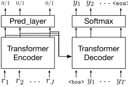
As presented before, we need to select the con-tent from the input records before generating the output summary. Some records are generally im-portant no mater the game context, such as the team name record and team score record, whereas the importance of some other records depend on the game context. For example, a player having the highest points in the game is more likely to be mentioned in the game summary. Within the Transformer architecture, the self-attention mech-anism can generate the latent representation for each record by jointly conditioning on all other records in the input dataset. A binary prediction layer is added on top of the Transformer encoder

output (as shown in Figure1) to predict whether

or not one record will be mentioned in the target summary.

The architecture of our data-to-text Transformer

model is shown in Figure 1. As presented

be-fore, the encoder takes the record embedding as input and generates the latent representation for each record in the input sequence. The output of encoder is then used to predict the importance of each record and also serves as the context of the decoder. The decoder of our model is the same as the original Transformer model in machine trans-lation. It predicts the next word conditioned on

the encoder output and the previous tokens in the summary sequence.

In content selection modeling, the input record sequences together with its label sequences are used to optimize the encoder by minimizing the cross-entropy loss. In language generation train-ing, the encoder and decoder are trained together to maximize the log-likelihood of the training data. The two learning objectives are trained

al-ternatively2_.

Transformer

Encoder

r

J

<latexit sha1_base64="JBdZO07IximDjYGIGbzvj4OxBGM=">AAAB6nicbVBNS8NAEJ34WetX1aOXxSJ4KkkV9Fj0Ip4q2g9oQ9lsJ+3SzSbsboQS+hO8eFDEq7/Im//GbZuDtj4YeLw3w8y8IBFcG9f9dlZW19Y3Ngtbxe2d3b390sFhU8epYthgsYhVO6AaBZfYMNwIbCcKaRQIbAWjm6nfekKleSwfzThBP6IDyUPOqLHSg+rd9Uplt+LOQJaJl5My5Kj3Sl/dfszSCKVhgmrd8dzE+BlVhjOBk2I31ZhQNqID7FgqaYTaz2anTsipVfokjJUtachM/T2R0UjrcRTYzoiaoV70puJ/Xic14ZWfcZmkBiWbLwpTQUxMpn+TPlfIjBhbQpni9lbChlRRZmw6RRuCt/jyMmlWK955pXp/Ua5d53EU4BhO4Aw8uIQa3EIdGsBgAM/wCm+OcF6cd+dj3rri5DNH8AfO5w8pvo23</latexit>

r

1

<latexit sha1_base64="w+fMBncFYKx0kEKsDtLgWG6j6to=">AAAB6nicbVBNS8NAEJ3Ur1q/qh69LBbBU0mqoMeiF48V7Qe0oWy2k3bpZhN2N0IJ/QlePCji1V/kzX/jts1BWx8MPN6bYWZekAiujet+O4W19Y3NreJ2aWd3b/+gfHjU0nGqGDZZLGLVCahGwSU2DTcCO4lCGgUC28H4dua3n1BpHstHM0nQj+hQ8pAzaqz0oPpev1xxq+4cZJV4OalAjka//NUbxCyNUBomqNZdz02Mn1FlOBM4LfVSjQllYzrErqWSRqj9bH7qlJxZZUDCWNmShszV3xMZjbSeRIHtjKgZ6WVvJv7ndVMTXvsZl0lqULLFojAVxMRk9jcZcIXMiIkllClubyVsRBVlxqZTsiF4yy+vklat6l1Ua/eXlfpNHkcRTuAUzsGDK6jDHTSgCQyG8Ayv8OYI58V5dz4WrQUnnzmGP3A+fwAD2o2e</latexit>

r

<latexit sha1_base64="qRYq8+LBOBKrAYqfcugvOTPcEds=">AAAB6nicbVBNS8NAEJ3Ur1q/qh69LBbBU0mqoMeiF48V7Qe0oWy2k3bpZhN2N0IJ/QlePCji1V/kzX/jts1BWx8MPN6bYWZekAiujet+O4W19Y3NreJ2aWd3b/+gfHjU0nGqGDZZLGLVCahGwSU2DTcCO4lCGgUC28H4dua3n1BpHstHM0nQj+hQ8pAzaqz0oPq1frniVt05yCrxclKBHI1++as3iFkaoTRMUK27npsYP6PKcCZwWuqlGhPKxnSIXUsljVD72fzUKTmzyoCEsbIlDZmrvycyGmk9iQLbGVEz0sveTPzP66YmvPYzLpPUoGSLRWEqiInJ7G8y4AqZERNLKFPc3krYiCrKjE2nZEPwll9eJa1a1buo1u4vK/WbPI4inMApnIMHV1CHO2hAExgM4Rle4c0Rzovz7nwsWgtOPnMMf+B8/gAFXo2f</latexit> 2

. . .

<latexit sha1_base64="D8NZwhGRc3SadH+lq9NyH2X2S6M=">AAAB7HicbVBNS8NAFHzxs9avqkcvi0XwVJIq6LHoxWMF0xbaUDbbTbt0swm7L0IJ/Q1ePCji1R/kzX/jts1BWwcWhpk37HsTplIYdN1vZ219Y3Nru7RT3t3bPzisHB23TJJpxn2WyER3Qmq4FIr7KFDyTqo5jUPJ2+H4bua3n7g2IlGPOEl5ENOhEpFgFK3k9wYJmn6l6tbcOcgq8QpShQLNfuXL5lgWc4VMUmO6nptikFONgkk+Lfcyw1PKxnTIu5YqGnMT5PNlp+TcKgMSJdo+hWSu/k7kNDZmEod2MqY4MsveTPzP62YY3QS5UGmGXLHFR1EmCSZkdjkZCM0ZyokllGlhdyVsRDVlaPsp2xK85ZNXSate8y5r9YerauO2qKMEp3AGF+DBNTTgHprgAwMBz/AKb45yXpx352MxuuYUmRP4A+fzB/K2jsY=</latexit>

Pred_layer

0/1

<latexit sha1_base64="TLXKA4mwwbXo2dx+G5FnabsZdt0=">AAAB6nicbVBNS8NAEJ34WetX1aOXxSJ4qkkV9Fj04rGi/YA2lM120y7dbMLuRCihP8GLB0W8+ou8+W/ctjlo64OBx3szzMwLEikMuu63s7K6tr6xWdgqbu/s7u2XDg6bJk414w0Wy1i3A2q4FIo3UKDk7URzGgWSt4LR7dRvPXFtRKwecZxwP6IDJULBKFrpwT33eqWyW3FnIMvEy0kZctR7pa9uP2ZpxBUySY3peG6CfkY1Cib5pNhNDU8oG9EB71iqaMSNn81OnZBTq/RJGGtbCslM/T2R0ciYcRTYzoji0Cx6U/E/r5NieO1nQiUpcsXmi8JUEozJ9G/SF5ozlGNLKNPC3krYkGrK0KZTtCF4iy8vk2a14l1UqveX5dpNHkcBjuEEzsCDK6jBHdShAQwG8Ayv8OZI58V5dz7mrStOPnMEf+B8/gBWT40s</latexit> 0<latexit sha1_base64="TLXKA4mwwbXo2dx+G5FnabsZdt0=">AAAB6nicbVBNS8NAEJ34WetX1aOXxSJ4qkkV9Fj04rGi/YA2lM120y7dbMLuRCihP8GLB0W8+ou8+W/ctjlo64OBx3szzMwLEikMuu63s7K6tr6xWdgqbu/s7u2XDg6bJk414w0Wy1i3A2q4FIo3UKDk7URzGgWSt4LR7dRvPXFtRKwecZxwP6IDJULBKFrpwT33eqWyW3FnIMvEy0kZctR7pa9uP2ZpxBUySY3peG6CfkY1Cib5pNhNDU8oG9EB71iqaMSNn81OnZBTq/RJGGtbCslM/T2R0ciYcRTYzoji0Cx6U/E/r5NieO1nQiUpcsXmi8JUEozJ9G/SF5ozlGNLKNPC3krYkGrK0KZTtCF4iy8vk2a14l1UqveX5dpNHkcBjuEEzsCDK6jBHdShAQwG8Ayv8OZI58V5dz7mrStOPnMEf+B8/gBWT40s</latexit> /1 0<latexit sha1_base64="TLXKA4mwwbXo2dx+G5FnabsZdt0=">AAAB6nicbVBNS8NAEJ34WetX1aOXxSJ4qkkV9Fj04rGi/YA2lM120y7dbMLuRCihP8GLB0W8+ou8+W/ctjlo64OBx3szzMwLEikMuu63s7K6tr6xWdgqbu/s7u2XDg6bJk414w0Wy1i3A2q4FIo3UKDk7URzGgWSt4LR7dRvPXFtRKwecZxwP6IDJULBKFrpwT33eqWyW3FnIMvEy0kZctR7pa9uP2ZpxBUySY3peG6CfkY1Cib5pNhNDU8oG9EB71iqaMSNn81OnZBTq/RJGGtbCslM/T2R0ciYcRTYzoji0Cx6U/E/r5NieO1nQiUpcsXmi8JUEozJ9G/SF5ozlGNLKNPC3krYkGrK0KZTtCF4iy8vk2a14l1UqveX5dpNHkcBjuEEzsCDK6jBHdShAQwG8Ayv8OZI58V5dz7mrStOPnMEf+B8/gBWT40s</latexit> /1

Transformer

Decoder

y

1

<latexit sha1_base64="gXLzr9lA6QyErQrPkt90wKdvXMk=">AAAB6nicbVBNS8NAEJ3Ur1q/qh69LBbBU0mqoMeiF48V7Qe0oWy2m3bpZhN2J0Io/QlePCji1V/kzX/jts1BWx8MPN6bYWZekEhh0HW/ncLa+sbmVnG7tLO7t39QPjxqmTjVjDdZLGPdCajhUijeRIGSdxLNaRRI3g7GtzO//cS1EbF6xCzhfkSHSoSCUbTSQ9b3+uWKW3XnIKvEy0kFcjT65a/eIGZpxBUySY3pem6C/oRqFEzyaamXGp5QNqZD3rVU0YgbfzI/dUrOrDIgYaxtKSRz9ffEhEbGZFFgOyOKI7PszcT/vG6K4bU/ESpJkSu2WBSmkmBMZn+TgdCcocwsoUwLeythI6opQ5tOyYbgLb+8Slq1qndRrd1fVuo3eRxFOIFTOAcPrqAOd9CAJjAYwjO8wpsjnRfn3flYtBacfOYY/sD5/AEOhI2l</latexit>

y

<latexit sha1_base64="JJSaiNpL04FogISMGU77Y0OBc24=">AAAB6nicbVBNS8NAEJ34WetX1aOXxSJ4KkkV9Fj04rFiv6ANZbOdtEs3m7C7EULpT/DiQRGv/iJv/hu3bQ7a+mDg8d4MM/OCRHBtXPfbWVvf2NzaLuwUd/f2Dw5LR8ctHaeKYZPFIladgGoUXGLTcCOwkyikUSCwHYzvZn77CZXmsWyYLEE/okPJQ86osdJj1m/0S2W34s5BVomXkzLkqPdLX71BzNIIpWGCat313MT4E6oMZwKnxV6qMaFsTIfYtVTSCLU/mZ86JedWGZAwVrakIXP198SERlpnUWA7I2pGetmbif953dSEN/6EyyQ1KNliUZgKYmIy+5sMuEJmRGYJZYrbWwkbUUWZsekUbQje8surpFWteJeV6sNVuXabx1GAUziDC/DgGmpwD3VoAoMhPMMrvDnCeXHenY9F65qTz5zAHzifP0OQjcg=</latexit> T

. . .

Softmax

. . .

y

<latexit sha1_base64="gXLzr9lA6QyErQrPkt90wKdvXMk=">AAAB6nicbVBNS8NAEJ3Ur1q/qh69LBbBU0mqoMeiF48V7Qe0oWy2m3bpZhN2J0Io/QlePCji1V/kzX/jts1BWx8MPN6bYWZekEhh0HW/ncLa+sbmVnG7tLO7t39QPjxqmTjVjDdZLGPdCajhUijeRIGSdxLNaRRI3g7GtzO//cS1EbF6xCzhfkSHSoSCUbTSQ9b3+uWKW3XnIKvEy0kFcjT65a/eIGZpxBUySY3pem6C/oRqFEzyaamXGp5QNqZD3rVU0YgbfzI/dUrOrDIgYaxtKSRz9ffEhEbGZFFgOyOKI7PszcT/vG6K4bU/ESpJkSu2WBSmkmBMZn+TgdCcocwsoUwLeythI6opQ5tOyYbgLb+8Slq1qndRrd1fVuo3eRxFOIFTOAcPrqAOd9CAJjAYwjO8wpsjnRfn3flYtBacfOYY/sD5/AEOhI2l</latexit> 1

y

<latexit sha1_base64="UmY8miGJFsYtImgQ4UOSFc3rPPg=">AAAB6nicbVBNS8NAEJ3Ur1q/qh69LBbBU0mqoMeiF48V7Qe0oWy2m3bpZhN2J0Io/QlePCji1V/kzX/jts1BWx8MPN6bYWZekEhh0HW/ncLa+sbmVnG7tLO7t39QPjxqmTjVjDdZLGPdCajhUijeRIGSdxLNaRRI3g7GtzO//cS1EbF6xCzhfkSHSoSCUbTSQ9av9csVt+rOQVaJl5MK5Gj0y1+9QczSiCtkkhrT9dwE/QnVKJjk01IvNTyhbEyHvGupohE3/mR+6pScWWVAwljbUkjm6u+JCY2MyaLAdkYUR2bZm4n/ed0Uw2t/IlSSIldssShMJcGYzP4mA6E5Q5lZQpkW9lbCRlRThjadkg3BW355lbRqVe+iWru/rNRv8jiKcAKncA4eXEEd7qABTWAwhGd4hTdHOi/Ou/OxaC04+cwx/IHz+QMQCI2m</latexit> 2 <eos>

<latexit sha1_base64="xDzQvAFdLmBTev1IjeBitAarx+g=">AAAB9XicbVDLSgNBEJyNrxhfUY9eBoPgKexGQQ8iQS8eI5gHJGuYnfQmQ2YfzPSqYcl/ePGgiFf/xZt/4yTZgyYWNBRV3XR3ebEUGm3728otLa+sruXXCxubW9s7xd29ho4SxaHOIxmplsc0SBFCHQVKaMUKWOBJaHrD64nffAClRRTe4SgGN2D9UPiCMzTSfQfhCRHTC4j05bhbLNllewq6SJyMlEiGWrf41elFPAkgRC6Z1m3HjtFNmULBJYwLnURDzPiQ9aFtaMgC0G46vXpMj4zSo36kTIVIp+rviZQFWo8Cz3QGDAd63puI/3ntBP1zNxVhnCCEfLbITyTFiE4ioD2hgKMcGcK4EuZWygdMMY4mqIIJwZl/eZE0KmXnpFy5PS1Vr7I48uSAHJJj4pAzUiU3pEbqhBNFnskrebMerRfr3fqYteasbGaf/IH1+QPyi5LM</latexit>

[image:3.595.306.523.208.356.2]

<bos><latexit sha1_base64="8AaeR7MZfhElgpaTf2flakQjM2E=">AAAB9XicbVBNSwMxEM3Wr1q/qh69BIvgqexWQQ8iRS8eK9gPaNeSTbNtaDZZklm1LP0fXjwo4tX/4s1/Y9ruQVsfDDzem2FmXhALbsB1v53c0vLK6lp+vbCxubW9U9zdaxiVaMrqVAmlWwExTHDJ6sBBsFasGYkCwZrB8HriNx+YNlzJOxjFzI9IX/KQUwJWuu8AewKA9CJQ5nLcLZbcsjsFXiReRkooQ61b/Or0FE0iJoEKYkzbc2PwU6KBU8HGhU5iWEzokPRZ21JJImb8dHr1GB9ZpYdDpW1JwFP190RKImNGUWA7IwIDM+9NxP+8dgLhuZ9yGSfAJJ0tChOBQeFJBLjHNaMgRpYQqrm9FdMB0YSCDapgQ/DmX14kjUrZOylXbk9L1assjjw6QIfoGHnoDFXRDaqhOqJIo2f0it6cR+fFeXc+Zq05J5vZR3/gfP4A7fOSyQ==</latexit>

Figure 1: Model Architecture

4 Data Augmentation Methods

In data-to-text generation task, the model needs to not only generate fluent text, but also generate text which is coherent with the input records. Several content-oriented evaluation metrics are proposed

in (Wiseman et al., 2017) to evaluate such

cohe-sion, including the precision of record generation and the recall rate with respect to the records in gold summary.

In this section, we present two data

augmenta-tion methods:synthetic data generationand

train-ing data selection. Each of them has different im-pacts on the content-oriented evaluation results.

4.1 Synthetic Data Generation

In order to improve the cohesion between the in-put records and outin-put summary, we need more data to enhance the encoder-decoder attention of the decoder. Here we introduce a method to gen-erate synthetic training data.

We first randomly change the values of records

and the changed record set (s0) is then used to

gen-erate automatic summary (t0) by a trained

data-to-text system. The synthetic data pairs (s0, t0) are

then used to improve such system.

2_{An alternative approach is joint training that achieves}

(4)

This idea is inspired by the back-translation technique widely used in neural machine transla-tion, with two important differences:

First, back-translation, typically employs

monolingual human texts, which are easy found. In our case, since it is difficult to find additional structured (table) data for the same kind of game matches, we use the existing data sets and intro-duce variations in the values of the table records. In order to keep the data cohesion in the table, the change is constrained with the following rules:

• only numeric values are changed.

Non-numeric values such as the position of a player or the city name of a team are kept the same.

• after the change, the team scores should not

violate the win/loss relation

• the changed values should stay in the normal

range of its value type. It should not bigger than its maximum value or smaller than its minimum value through all games.

Our data generation technique doubles the amount of training data available for learning.

Second, another difference with the

back-translation technique is the “translation

direc-tion”. In machine translation, the additional

monolingual text used is found in target guage, and back-translated into the source lan-guage. Thus, ensuring that the target side of the synthetic data follows the same distribution as real human texts. In our case, the target side of syn-thetic data is also automatically generated which is known to introduce noise in the resulting net-work.

4.2 Training Data Selection

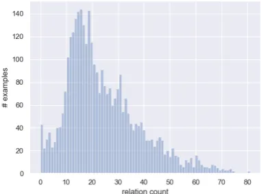
A deficiency of data-to-text NLG systems is the poor coverage of relations produced in the gener-ated summaries. In order to increase the coverage, a simple solution consists of learning to produce a larger number of relations. Here, we present a straightforward method to bias our model to out-put more relations by means of fine-tuning on the training examples containing a greater number of relations.

We use an information extraction (IE) system to extract the number of relations of each train-ing summary. Then, we select for fine-tuntrain-ing our baseline model the subset of training data in which

each summary contains at least N relations. In

this work, we take advantage of the IE system3

provided by (Puduppully et al.,2019), and the

dis-tribution of the number of relations in the training

[image:4.595.313.504.163.305.2]

summary is illustrated in Figure2.

Figure 2: relation count distribution in training data.

5 Experimental Setup

5.1 Data and Preprocessing

We run the experiments with the ROTOWIRE

dataset (Wiseman et al.,2017), a dataset of NBA

basketball game summaries, paired with their

cor-responding box- and line-score tables. Table1

il-lustrates an example of the dataset. In the box-score table, each team has at most 13 players and each player is described by 23 types of values. In the line-score table, each team has 15 differ-ent types of values. In addition, the date of each game is converted into the day of the week (such as “Saturday”) as an additional record. In the pre-processing step, the input box- and line-score ta-bles are converted into a fix-length sequence of

records. Each sequence contains 629 records.4 As

for the associate summaries, the average length is 337 tokens, and the vocabulary size is 11.3K. The

ROTOWIRE dataset contains 4853 summaries in

total, in which 3398 summaries are for training, 727 for validation and 728 for test.

In content selection modelling, we need the la-bels of input records to indicate which records in the input will be mentioned in the output sum-mary. Here we use a very simple method to

gener-3

The model is publicly available athttps://github.

com/ratishsp/data2text-plan-py

4_{In the 629 records, 598 records are for players, 30}

(5)

NAME POS MIN PTS FGM FGA FG PCT FG3M FG3A FG3 PCT FTM FTA FT PCT OREB DREB REB AST TO STL BLK PF

Matt Barnes F 26 0 0 3 0 0 3 0 0 0 0 1 4 5 4 1 0 0 0

Blake Griffin F 34 24 10 17 59 0 0 0 4 5 80 4 2 6 8 4 1 0 3

DeAndre Jordan C 34 9 4 8 50 0 0 0 1 4 25 5 11 16 0 1 1 2 4

JJ Redick G 34 23 9 15 60 5 8 63 0 0 0 0 3 3 2 1 1 0 2

Chris Paul G 36 27 6 16 38 4 6 67 11 12 92 1 2 3 9 2 2 1 3

Glen Davis N/A 13 2 1 2 50 0 0 0 0 0 0 0 4 4 1 0 3 0 0

Jamal Crawford N/A 29 17 5 16 31 3 8 38 4 6 67 0 2 2 2 1 2 1 2

Hedo Turkoglu N/A 6 0 0 0 0 0 0 0 0 0 0 0 2 2 0 1 0 0 1

Reggie Bullock N/A 14 2 1 1 100 0 0 0 0 0 0 0 0 0 1 0 0 0 0

Jordan Farmar N/A 12 2 1 3 33 0 1 0 0 0 0 0 0 0 2 1 0 0 3

Jared Cunningha N/A N/A N/A N/A N/A N/A N/A N/A N/A N/A N/A N/A N/A N/A N/A N/A N/A N/A N/A N/A Chris Douglas-R N/A N/A N/A N/A N/A N/A N/A N/A N/A N/A N/A N/A N/A N/A N/A N/A N/A N/A N/A N/A Ekpe Udoh N/A N/A N/A N/A N/A N/A N/A N/A N/A N/A N/A N/A N/A N/A N/A N/A N/A N/A N/A N/A

Giannis Antetok F 38 18 8 12 67 0 1 0 2 3 67 1 8 9 6 3 2 0 3

Johnny O’Bryant F 6 4 2 3 67 0 0 0 0 0 0 0 0 0 0 0 0 0 2

Larry Sanders C 26 10 5 6 83 0 0 0 0 2 0 2 5 7 3 0 1 1 5

O.J. Mayo G 23 3 1 6 17 0 2 0 1 3 33 0 1 1 3 2 0 0 4

Brandon Knight G 27 8 3 10 30 2 6 33 0 0 0 1 4 5 5 4 0 0 3

Jared Dudley N/A 30 16 7 12 58 2 4 50 0 0 0 2 6 8 3 3 2 0 2

Zaza Pachulia N/A 20 5 1 3 33 0 0 0 3 4 75 2 5 7 2 2 0 0 1

Jerryd Bayless N/A 28 16 7 13 54 2 3 67 0 0 0 1 3 4 2 1 0 0 4

Khris Middleton N/A 24 12 5 10 50 1 5 20 1 1 100 1 3 4 2 0 1 0 2

Kendall Marshal N/A 18 10 4 6 67 1 3 33 1 2 50 0 1 1 3 3 0 0 0

Damien Inglis N/A N/A N/A N/A N/A N/A N/A N/A N/A N/A N/A N/A N/A N/A N/A N/A N/A N/A N/A N/A Jabari Parker N/A N/A N/A N/A N/A N/A N/A N/A N/A N/A N/A N/A N/A N/A N/A N/A N/A N/A N/A N/A Nate Wolters N/A N/A N/A N/A N/A N/A N/A N/A N/A N/A N/A N/A N/A N/A N/A N/A N/A N/A N/A N/A

TEAM-NAME CITY P QTR1 P QTR2 P QTR3 P QTR4 PTS FG PCT FG3 PCT FT PCT REB AST TOV WINS LOSSES

Clippers Los Angeles 28 22 32 24 106 46 46 74 41 29 12 19 8

Bucks Milwaukee 24 28 31 19 102 53 33 53 46 29 18 14 14

[image:5.595.78.535.60.306.2]

The Los Angeles Clippers (19-8) defeated the Milwaukee Bucks (14-14) 106-102 on Saturday. Los Angeles has won three of their last four games. Chris Paul paced the team with a game-high 27 points and nine assists. DeAndre Jordan continued his impressive work on the boards, pulling down 16 rebounds, and Blake Griffin and J.J. Redick joined Paul in scoring over 20 points. The Clippers have a tough stretch of their schedule coming up with the Spurs, Hawks, Warriors and Raptors all on this week’s docket. Even with the loss, Milwaukee finished their four-game Western Conference road trip 2-2, a job well done by the developing squad. In the three games since Jabari Parker went down with a season-ending ACL injury, coach Jason Kidd has cut the umbilical cord they had on Giannis Antetokounmpo. He played over 37 minutes for the second straight game Saturday, which is ten more minutes than his season average of 27 minutes per game. Larry Sanders returned to the starting lineup after sitting out Thursday’s game on a league mandated one-game suspension. Ersan Ilyasova (concussion) and John Henson (foot) remain out, and it seems Ilyasova may be closer to returning than Henson.

Table 1: An example of box-score (top), line-score (middle) and the corresponding summary (bottom) from ROTOWIREdataset. The definition of table header could be found athttps://github.com/harvardnlp/ boxscore-data

ate such labels. First, we label the entity records5.

An entity record is labeled as1if its value is

men-tioned in the associated summary, otherwise it is

labeled as0. Second, for each player or team

[image:5.595.75.538.61.308.2]

men-tioned in the summary, the rest of its values in the

table are labeled as1if they occur in the same

sen-tence in the summary.

5.2 Evaluation metrics

The model output is evaluated with BLEU

(Pa-pineni et al., 2002) as well as several

content-oriented metrics proposed by (Wiseman et al., 2017) including three following aspects:

5_{Record whose}

Valuefeature is an entity (see Section3),

for example: “LeBron James|NAME|LeBron James|H/W”.

The labeling is according to theValuefeature

• Relation Generation (RG) evaluates the

num-ber of extracted relations in automatic sum-maries and their correctness (precision) w.r.t the input record dataset;

• Content Selection (CS) evaluates the

preci-sion and recall rate of extracted relations in automatic summaries w.r.t that in the gold summaries;

• Content Ordering (CO) evaluates the

normal-ized Damerau-Levenshtein Distance (Brill

and Moore, 2000) between the sequence of

extracted relations in automatic summaries and that in the gold summaries.

(6)

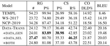
Model RG CS CO BLEU

# P% P% R% DLD%

[image:6.595.73.288.60.159.2]

GOLD 23.32 94.77 100 100 100 100 TEMPL 54.29 99.92 26.61 59.16 14.42 8.51 WS-2017 23.95 75.10 28.11 35.86 15.33 14.57 NCP-2019 33.88 87.51 33.52 51.21 18.57 16.19 DATA-TRANS 23.31 79.81 36.90 43.06 22.75 20.60 +DATA GEN 22.59 82.49 39.48 42.84 23.32 19.76 +DATA SEL 26.94 79.54 35.27 47.49 22.22 19.97 +BOTH 24.24 80.52 37.33 44.66 23.04 20.22

Table 2: Automatic evaluation on ROTOWIRE devel-opment set using relation generation (RG) count (#) and precision (P%), content selection (CS) precision (P%) and recall (R%), content ordering (CO) in nor-malized Damerau-Levenshtein distance (DLD%), and BLEU.

summaries. For the purpose of comparison, we directly use the publicly available IE system of

(Puduppully et al.,2019) to evaluate our models.

5.3 Training Details

In all experiments, we use our model with 1 en-coder layer and 6 deen-coder layers, 512 hidden units (hence, the record feature embedding size

is 128, see Section 3), 8 heads, GELU

activa-tions (Hendrycks and Gimpel, 2016), a dropout

rate of 0.1 and learned positional embedding for the decoder. The model is trained with the Adam

optimizer (Kingma and Ba,2014), learning rate is

fixed to10−4_{and batch size is 6. As for inference,}

we use beam size 4 for all experiments, and the maximum decoding length is 600.

We implement all our models in Pytorch, and train them on 1 GTX 1080 GPU.

6 Results

The results of our model on the development

set are summarized in Table 2. GOLD

repre-sents the evaluation result on the gold summary. The RG precision rate is 94.77%, indicating that the IE system for evaluation is not perfect but

has very high precision. After that, results of

three contrast systems are reported, where TEMPL

and WS-2017 are the updated results6 of

Wise-man et al. (2017) models. TEMPL is

template-based generator model which generates a sum-mary consisting of 8 sentences: a general de-scription sentence about the teams playing in the game, 6 player-specific sentences and a conclusion sentence. WS-2017 reports an encoder-decoder

6_{Here we all use the IE system of (}_{Puduppully et al.}_,₂₀₁₉₎

which is improved from the original IE system of (Wiseman

et al.,2017)

model with conditional copy mechanism. NCP-2019 is the best system configuration (NCP+CC)

reported in (Puduppully et al., 2019) which is a

neural content planning model enhanced with con-ditional copy mechanism. As for our model, re-sults with four configurations are reported.

DATA-TRANS represents our data-to-text

Transformer model (as illustrated in Figure 1)

without any data augmentation. Comparing to

NCP-2019, our model performs 3.4% higher on content selection precision, 4.2% higher on content ordering metric and 4.4 points higher on BLEU. Our model performs better on the CO metric, we attribute this improvement to that our model generates nearly the same number of relations as the gold summary which reduces the edit distance between the two sequences of relations. However, our model is 7.7% lower on

RG precision. And on the CS recall rate, our

model is 8.2% lower than NCP-2019. This is probably due to the fact that NCP-2019 generates much more records than our model (33.88 vs. 23.31) which could result higher coverage on the relations in gold summary.

Comparing to TEMPL and WS-2017, our

model is much better on BLEU and CS precision. Our model generates nearly the same number of relations as WS-2017, but with 7.2% higher on recall rate and 7.4% higher on CO metric.

By synthetic data generation (+DATA GEN), we generate synthetic table records as described in

se-cion 4.1. These synthetic table records are then

used as input to the DATA-TRANSmodel to

gener-ate summaries. All training table records are used to generate synthetic data. The synthetic data is then combined with the original training data to

fine-tune the DATA-TRANSmodel. From Table2,

we can see that the RG and CS precisions are both improved by 2.7% and 2.6% respectively. There is no significant change on others metrics. The CO metric is slightly improved due to higher RG and CS precisions. The CS recall rate is slightly de-graded with the number of extracted relations.

By training data selection (+DATA SEL), we se-lect the data whose summary contains the

num-ber of relations N >= 16 as the new training

data. The result training data size is 2242 (original size: 3398). It is then used to fine-tune the

DATA-TRANSmodel. As shown in Table2, as expected,

(7)

num-Model RG CS CO BLEU

# P% P% R% DLD%

[image:7.595.74.288.61.150.2]

TEMPL 54.23 99.94 26.99 58.16 14.92 8.46 WS-2017 23.72 74.80 29.49 36.18 15.42 14.19 NCP-2019 34.28 87.47 34.18 51.22 18.58 16.50 DATA-TRANS 24.12 79.17 36.48 42.74 22.40 20.16 +DATA GEN 24.01 83.89 38.98 42.85 23.02 19.48 +DATA SEL 27.47 80.70 35.33 46.25 21.87 20.03 +BOTH 24.80 81.08 37.10 43.78 22.51 20.14

Table 3: Automatic evaluation on ROTOWIREtest set.

Model RG CS CO BLEU

# P% P% R% DLD%

DATA-TRANS 23.31 79.81 36.90 43.06 22.75 20.60 -CS OBJ 23.37 72.70 32.67 41.99 21.14 20.28 -REC EMB 18.00 63.14 32.94 37.71 21.15 20.24

Table 4: Ablation results on ROTOWIREdev set.

ber of relations in the output summaries increases from 23.31 to 26.94. Respectively, the CS recall is increased from 43.06% to 47.49%. However, the CS precision is slightly degraded by 1.6%.

Finally, we combine both of the data augmen-tation methods (+BOTH). Synthetic data genera-tion improves the RG and CS precisions. Train-ing data selection improves the CS recall rate by

making the model generate more relations. To

combine the two methods, we choose to fine-tune

the +DATA GEN model with the selected

train-ing data of +DATA SEL (so this configuration is

actually +DATA GEN+DATA SEL). As shown in

Table 2, all content-oriented evaluation metrics

are improved compared to DATA-TRANS but not

as much as each single of the data augmentation method. This configuration is like a trade-off be-tween the two data augmentation configurations.

Results on the test set are reported in Table 3.

They follow the same pattern as those found on

the development set. Our DATA-TRANS model

outperforms all other contrast systems on BLEU, CS precision and content ordering metrics. The synthetic data generation method helps to improve the RG and CS precisions. The training data se-lection method improves the CS recall by mak-ing the model generate more relations. Combinmak-ing these two data augmentation methods, all content-oriented evaluation results are improved compared to DATA-TRANS. However, there is no significant change on BLEU.

7 Ablation Experiments

Next we evaluate the extensions introduced in our data-to-text Transformer model (DATA-TRANS) by means of ablation experiments. This is:

• The concatenation of feature embeddings as

input of the encoder presented in Section3.1

in order to generate a better representation of the input records.

• The secondary learning objective presented

in Sectioin 3.2 aiming at improving the

content-oriented results.

Removing the content selection additional

ob-jective function In this configuration, we keep

the same data embedding and the model architec-ture as the DATA-TRANS, but the model is trained without the content selection objective. The

eval-uation results are shown in Table4(-CS OBJ). We

can see that the CS precision and CS recall are de-graded by 4.2% and 1% respectively. The model extracts nearly the same number of records as the baseline system, but with much lower precision. The content ordering metric is also degraded by 1.6%. Surprisingly, there is no significant change on BLEU.

Removing Record Encoding In this

configu-ration, the record encoding is removed from the

DATA-TRANSmodel. Instead, we directly use the

Value feature (see Section 3) sequence as the

in-put. To keep model size unchanged, the

dimen-sion of embedding for theValuefeature sequence

is four times bigger than the original feature

em-bedding size (see Equation2). In addition, we also

add back the positional embedding for the input sequence. Since the record sequence has a fixed length of 629, the positional embedding could help to build a 1-to-1 mapping from the position in record sequence and the position in the real table.

The model is trained with the same data and the same configuration as DATA-TRANS. From the

re-sults in Table4(-REC EMB), we can see that

with-out record embedding all content-oriented evalu-ation results are degraded, especially the RG pre-cision and CS recall. And again, the model still achieves comparable BLEU score with

DATA-TRANS which demonstrates the effectiveness of

Transformer model on language modeling.

An example output of -REC EMB system is

shown in Table5(left). The generation has high

precision at the beginning, and many erroneous re-lations are generated after several sentences. Our

DATA-TRANS performs much better, but we can

(8)

The Los Angeles Clippers (19-8) defeated the Milwaukee Bucks (14-14) 106-102 on Saturday. Milwaukee has won four straight games.They were paced by J.J. Redick’s game with 23 points,five assists and five rebounds. Chris Paul had a nice game with 27 points and nine assists to go along with a double-double withnine pointsand nine assists. The Clippers shot53 percent from the fieldand 46 percent from beyond the arc. Milwaukee will wrap up their two-game road trip

in Houston against the Grizzlies on Tuesday.Milwaukee has

lost four straight games. They’ve lost five of their last five games. Chris Paul (ankle) and Blake Griffin (knee) sat out Saturday’s game. The Clippers missed their last two games

with a hamstring strain. Jordan had to leave the lead the team with a foot injury but were able to return for the Clippers to action on Friday.

The Los Angeles Clippers (19-8) defeated the Milwaukee Bucks (14-14) 106-102 on Saturday. Los Angeles stopped

their two-game losing streak with the win. Jamal Crawford

paced the team with a game-high 17 points in 29 minutes off the bench. Crawford shot9-of-16 from the field and 3-of-8 from downtown. He hadnine assists, two rebounds and two steals in 29 minutes. Blake Griffin had 24 points, eight as-sists, six rebounds and one steal in 34 minutes.The Clippers will go on the road to face the Denver Nuggets on Monday. Milwaukee has lost two straight, and are now 9-2 in their last

10 games. Jabari Parker (ankle) didn’t play Saturday as he

recorded a double-double with18 pointsandnine rebounds.

Giannis Antetokounmpo (8-12 FG,2-1 3Pt, 2-3 FT) and nine rebounds in 38 minutes off the bench.The Clippers will stay home and host the Brooklyn Nets on Monday.

Table 5: Example output from DATA-TRANS (right) and ablation model -REC EMB (left). The corresponding box- and line-table are given in Table1. Text that accurately reflects a record in the associated table data is inblue, erroneous text is inred. Text in black is not contradictory to the table records and text inorangeis self-contradictory within the summary.

caused by the error accumulation effect in autore-gressive decoding.

Another problem we have observed, not only

in Table 5but also in other output summaries, is

repetition and self-contradictory. In the left

ex-ample of Table 5, it contains two sentences (in

orange color) which are completely contradictory with each other. And in the right example, the sen-tence in orange color contains contradictory infor-mation within the sentence.

8 Conclusions

We presented a Transformer-based data-to-text

generation model. Experimental results have

shown that our two modifications on the Trans-former model significantly improve the content-oriented evaluation metrics. In addition, we pro-posed two data augmentation methods, each of them improves different aspects of the model. Our final model outperforms current state-of-the-art system on BLEU, content selection precision and content ordering metics. And we believe it has great potential for the future work. In the next step, we would like to apply some experimental tech-niques of machine translation such as right-to-left decoding and system ensemble to the data-to-text generation task.

References

Gabor Angeli, Percy Liang, and Dan Klein. 2010. A simple domain-independent probabilistic approach to generation. InProceedings of the 2010 Confer-ence on Empirical Methods in Natural Language Processing, pages 502–512. Association for Com-putational Linguistics.

Regina Barzilay and Mirella Lapata. 2005. Collective content selection for concept-to-text generation. In Proceedings of the conference on Human Language Technology and Empirical Methods in Natural Lan-guage Processing, pages 331–338. Association for Computational Linguistics.

Eric Brill and Robert C Moore. 2000. An improved er-ror model for noisy channel spelling correction. In Proceedings of the 38th Annual Meeting on Associa-tion for ComputaAssocia-tional Linguistics, pages 286–293. Association for Computational Linguistics.

Pablo A Duboue and Kathleen R McKeown. 2001. Empirically estimating order constraints for content planning in generation. InProceedings of the 39th Annual Meeting on Association for Computational Linguistics, pages 172–179. Association for Com-putational Linguistics.

Pablo A Duboue and Kathleen R McKeown. 2003. Sta-tistical acquisition of content selection rules for nat-ural language generation. In Proceedings of the 2003 conference on Empirical methods in natural language processing, pages 121–128. Association for Computational Linguistics.

(9)

Caglar Gulcehre, Sungjin Ahn, Ramesh Nallap-ati, Bowen Zhou, and Yoshua Bengio. 2016. Pointing the unknown words. arXiv preprint arXiv:1603.08148.

Dan Hendrycks and Kevin Gimpel. 2016. Bridging nonlinearities and stochastic regularizers with gaus-sian error linear units.

Diederik P Kingma and Jimmy Ba. 2014. Adam: A method for stochastic optimization. arXiv preprint arXiv:1412.6980.

Ioannis Konstas and Mirella Lapata. 2012. Unsuper-vised concept-to-text generation with hypergraphs. InProceedings of the 2012 Conference of the North American Chapter of the Association for Computa-tional Linguistics: Human Language Technologies, pages 752–761. Association for Computational Lin-guistics.

R´emi Lebret, David Grangier, and Michael Auli. 2016. Neural text generation from structured data with ap-plication to the biography domain. arXiv preprint arXiv:1603.07771.

Percy Liang, Michael I Jordan, and Dan Klein. 2009. Learning semantic correspondences with less super-vision. InProceedings of the Joint Conference of the 47th Annual Meeting of the ACL and the 4th Interna-tional Joint Conference on Natural Language Pro-cessing of the AFNLP: Volume 1-Volume 1, pages 91–99. Association for Computational Linguistics.

Hongyuan Mei, Mohit Bansal, and Matthew R Walter. 2015. What to talk about and how? selective gen-eration using lstms with coarse-to-fine alignment. arXiv preprint arXiv:1509.00838.

Kishore Papineni, Salim Roukos, Todd Ward, and Wei-Jing Zhu. 2002. Bleu: a method for automatic eval-uation of machine translation. In Proceedings of the 40th annual meeting on association for compu-tational linguistics, pages 311–318. Association for Computational Linguistics.

Ratish Puduppully, Li Dong, and Mirella Lapata. 2019. Data-to-text generation with content selection and planning. In Proceedings of the AAAI Conference on Artificial Intelligence, volume 33, pages 6908– 6915.

Ehud Reiter and Robert Dale. 1997. Building applied natural language generation systems. Natural Lan-guage Engineering, 3(1):57–87.

Ehud Reiter, Somayajulu Sripada, Jim Hunter, Jin Yu, and Ian Davy. 2005. Choosing words in computer-generated weather forecasts. Artificial Intelligence, 167(1-2):137–169.

Amanda Stent, Rashmi Prasad, and Marilyn Walker. 2004. Trainable sentence planning for complex in-formation presentation in spoken dialog systems. In Proceedings of the 42nd annual meeting on associa-tion for computaassocia-tional linguistics, page 79. Associ-ation for ComputAssoci-ational Linguistics.

Kumiko Tanaka-Ishii, Kˆoiti Hasida, and Itsuki Noda. 1998. Reactive content selection in the generation of real-time soccer commentary. InProceedings of the 17th international conference on Computational linguistics-Volume 2, pages 1282–1288. Association for Computational Linguistics.

Ashish Vaswani, Noam Shazeer, Niki Parmar, Jakob Uszkoreit, Llion Jones, Aidan N Gomez, Łukasz Kaiser, and Illia Polosukhin. 2017. Attention is all you need. InAdvances in neural information pro-cessing systems, pages 5998–6008.

Sam Wiseman, Stuart M Shieber, and Alexander M Rush. 2017. Challenges in data-to-document gen-eration. arXiv preprint arXiv:1707.08052.