Proceedings of the 2011 Conference on Empirical Methods in Natural Language Processing, pages 1500–1511,
Structured Sparsity in Structured Prediction
Andr´e F. T. Martins∗† Noah A. Smith∗ Pedro M. Q. Aguiar‡ M´ario A. T. Figueiredo† ∗School of Computer Science, Carnegie Mellon University, Pittsburgh, PA 15213, USA
‡Instituto de Sistemas e Rob´otica, Instituto Superior T´ecnico, Lisboa, Portugal †Instituto de Telecomunicac¸˜oes, Instituto Superior T´ecnico, Lisboa, Portugal
{afm,nasmith}@cs.cmu.edu, [email protected], [email protected]
Abstract
Linear models have enjoyed great success in structured prediction in NLP. While a lot of progress has been made on efficient train-ing with several loss functions, the problem of endowing learners with a mechanism for feature selection is still unsolved. Common approaches employ ad hoc filtering or L1 -regularization; both ignore the structure of the feature space, preventing practicioners from encoding structural prior knowledge. We fill this gap by adopting regularizers that promote
structured sparsity, along with efficient algo-rithms to handle them. Experiments on three tasks (chunking, entity recognition, and de-pendency parsing) show gains in performance, compactness, and model interpretability.
1 Introduction
Models for structured outputs are in demand across natural language processing, with applications in in-formation extraction, parsing, and machine transla-tion. State-of-the-art models usually involve linear combinations of features and are trained discrim-inatively; examples are conditional random fields (Lafferty et al., 2001), structured support vector machines (Altun et al., 2003; Taskar et al., 2003; Tsochantaridis et al., 2004), and the structured per-ceptron (Collins, 2002a). In all these cases, the un-derlying optimization problems differ only in the choice of loss function; choosing among them has usually a small impact on predictive performance.
In this paper, we are concerned with model se-lection: which features should be used to define the prediction score? The fact that models with few features (“sparse” models) are desirable for several
reasons (compactness, interpretability, good gener-alization) has stimulated much research work which has produced a wide variety of methods (Della Pietra et al., 1997; Guyon and Elisseeff, 2003; McCallum, 2003). Our focus is on methods which embed this selection into the learning problem via the regular-ization term. We depart from previous approaches in that we seek to make decisions jointly about all candidate features, and we want to promote sparsity patterns that go beyond the mere cardinality of the set of features. For example, we want to be able to select entire feature templates(rather than features individually), or to make the inclusion of some fea-tures depend on the inclusion of other feafea-tures.
We achieve the goal stated above by employ-ing regularizers which promotestructured sparsity. Such regularizers are able to encode prior knowl-edge and guide the selection of features by model-ing the structure of the feature space. Lately, this type of regularizers has received a lot of attention in computer vision, signal processing, and compu-tational biology (Zhao et al., 2009; Kim and Xing, 2010; Jenatton et al., 2009; Obozinski et al., 2010; Jenatton et al., 2010; Bach et al., 2011). Eisenstein et al. (2011) employed structured sparsity in com-putational sociolinguistics. However, none of these works have addressed structured prediction. Here, we combine these two levels of structure: struc-ture in the output space, and strucstruc-ture in the feastruc-ture space. The result is a framework that allows build-ing structured predictors with high predictive power, while reducing manual feature engineering. We ob-tain models that are interpretable, accurate, and of-ten much more compact than L2-regularized ones.
Compared withL1-regularized models, ours are
2 Structured Prediction
We address structured prediction problems, which involve an input setX(e.g., sentences) and an
out-put setY, assumed large and structured (e.g., tags or
parse trees). We assume that eachx ∈ Xhas a set
of candidate outputsY(x) ⊆Y. We consider linear
models, in which predictions are made according to
b
y= arg maxy∈Y(x)θ·φ(x, y), (1)
whereφ(x, y)∈RDis a vector of features, andθ∈ RDis the vector of corresponding weights. LetD=
{hxi, yii}Ni=1be a training sample. We assume a cost
function is defined such that c(y, yb ) is the cost of predictingybwhen the true output isy; our goal is to learnθwith small expected cost on unseen data. To achieve this goal, linear models are usually trained by solving a problem of the form
b
θ= arg minθΩ(θ) + N1 PNi=1L(θ, xi, yi), (2)
where Ω is a regularizer and L is a loss function. Examples of losses are: the negative conditional log-likelihood used in CRFs (Lafferty et al., 2001),
LCRF(θ, x, y) =−logPθ(y|x), (3)
where Pθ(y|x) ∝ exp(θ ·φ(x, y))is a log-linear model; the margin rescaled loss of structured SVMs (Taskar et al., 2003; Tsochantaridis et al., 2004),
LSVM(θ, x, y) = max
y0∈Y(x)θ·δφ(y
0) +c(y0, y), (4)
whereδφ(y0) =φ(x, y0)−φ(x, y); and the loss un-derlying the structured perceptron (Collins, 2002a),
LSP(θ, x, y) = maxy0∈Y(x)θ·δφ(y0). (5)
Empirical comparison among these loss functions can be found in the literature (see,e.g., Martins et al., 2010, who also consider interpolations of the losses above). In practice, it has been observed that the choice of loss has far less impact than the model de-sign and choice of features. Hence, in this paper, we focus our attention on the regularization term in Eq. 2. We specifically address ways in which this term can be used to help design the model by pro-moting structured sparsity. While this has been a topic of intense research in signal processing and
computational biology (Jenatton et al., 2009; Liu and Ye, 2010; Bach et al., 2011), it has not yet re-ceived much attention in the NLP community, where the choice of regularization for supervised learning has essentially been limited to the following:
• L2-regularization (Chen and Rosenfeld, 2000):
ΩL2
λ (θ) , λ2kθk22 = λ2 PD
d=1θ2d; (6)
• L1-regularization (Kazama and Tsujii, 2003;
Goodman, 2004):
ΩL1
τ (θ) , τkθk1 = τPDd=1|θd|. (7)
The latter is known as “Lasso,” as popularized by Tibshirani (1996) in the context of sparse regres-sion. In the two cases above, λandτ are nonneg-ative coefficients controlling the intensity of the reg-ularization.ΩL2
λ usually leads to easier optimization
and robust performance; ΩL1
τ encourages sparser
models, where only a few features receive nonzero weights; see Gao et al. (2007) for an empirical com-parison. More recently, Petrov and Klein (2008b) applied L1 regularization for structure learning in
phrase-based parsing; a comparison withL2appears
in Petrov and Klein (2008a). Elastic nets interpolate betweenL1 andL2, having been proposed by Zou
and Hastie (2005) and used by Lavergne et al. (2010) to regularize CRFs.
Neither of the regularizers just described “looks” at thestructure of the feature space, since they all treat each dimension independently—we call them
unstructured regularizers, as opposed to the struc-tured ones that we next describe.
3 Structured Sparsity
We are interested in regularizers that share withΩL1
τ
the ability to promote sparsity, so that they can be used for selecting features. In addition, we want to endow the feature space RD with additional
struc-ture, so that features are not penalized individually (as in theL1-case) but collectively, encouraging
3.1 The Group Lasso
To capture the structure of the feature space, we group ourD features intoM groupsG1, . . . , GM,
where each Gm ⊆ {1, . . . , D}. Ahead, we
dis-cuss meaningful ways of choosing group decompo-sitions; for now, let us assume a sensible choice is obvious to the model designer. Denote by θm =
hθdid∈Gm the subvector of those weights that
cor-respond to the features in the m-th group, and let d1, . . . , dM be nonnegative scalars (one per group).
We consider the followinggroup-Lassoregularizers:
ΩGL
d =
PM
m=1dmkθmk2. (8)
These regularizers were first proposed by Bakin (1999) and Yuan and Lin (2006) in the context of re-gression. Ifd1 =. . . =dM,ΩGLd becomes the “L1
norm of the L2 norms.” Interestingly, this is also
a norm, called the mixedL2,1-norm.1 These
regu-larizers subsume theL1 andL2 cases, which
corre-spond to trivial choices of groups:
• If each group is a singleton, i.e., M = D and Gd={θd}, andd1 =. . .=dM =τ, we recover
L1-regularization (cf. Eqs. 7–8).
• If there is a single group spanning all the features, i.e.,M = 1andG1 ={1, . . . , D}, then the right
hand side of Eq. 8 becomesd1kθk2. This is
equiv-alent toL2regularization.2
We next present some non-trivial examples con-cerning different topologies ofG={G1, . . . , GM}.
Non-overlapping groups. Let us first consider the case where G is a partition of the feature
space: the groups cover all the features (SmGm =
{1, . . . , D}), and they do not overlap (Ga∩Gb =∅,
∀a 6= b). Then, ΩGLd is termed anon-overlapping
group-Lassoregularizer. It encourages sparsity pat-terns in which entire groups are discarded. A ju-dicious choice of groups can lead to very compact
1In the statistics literature, such mixed-norm regularizers, which group features and then apply a separate norm for each group, are called composite absolute penalties (Zhao et al., 2009); other norms besidesL2,1 can be used, such asL∞,1
(Quattoni et al., 2009; Wright et al., 2009; Eisenstein et al., 2011).
2Note that Eqs. 8 and 6 do not becomeexactlythe same: in Eq. 6, theL2 norm is squared. However it can be shown that
both regularizers lead to identical learning problems (Eq. 2) up to a transformation of the regularization constant.
models and pinpoint relevant groups of features. The following examples lie in this category:
• The two cases above (L1 andL2 regularization). • Label-based groups. In multi-label classification,
whereY ={1, . . . , L}, features are typically de-signed as conjunctions of input features with la-bel indicators, i.e., they take the formφ(x, y) = ψ(x)⊗ey, whereψ(x)∈RDX,ey ∈RLhas all
entries zero except they-th entry, which is1, and ⊗denotes the Kronecker product. Henceφ(x, y) can be reshaped as aDX-by-Lmatrix, and we can
let each group correspond to a row. In this case, all groups have the same size and we typically set d1 = . . . = dM. A similar design can be made
for sequence labeling problems, by considering a similar grouping for the unigram features.3
• Template-based groups. In NLP, features are
com-monly designed via templates. For example, a template such asw0∧p0∧p−1denotes the word
in the current position (w0) conjoined with its
part-of-speech (p0) and that of the previous word
(p−1). This template encloses many features
cor-responding to different instantiantions of w0, p0,
andp−1. In§5, we learnfeature templatesfrom
the data, by associating each group to a feature template, and letting that group contain all fea-tures that are instantiations of this template. Since groups have different sizes, it is a good idea to letdmincrease with the group size, so that larger
groups pay a larger penalty for being included. Tree-structured groups. More generally, we may let the groups inGoverlap but be nested,i.e., we may
want them to form ahierarchy(two distinct groups either have empty intersection or one is contained in the other). This induces a partial order onG(the set
inclusion relation⊇), endowing it with the structure of a partially ordered set (poset).
A convenient graphical representation of the poset
hG,⊇i is itsHasse diagram. Each group is a node in the diagram, and an arc is drawn from groupGa
to group Gb if Gb ⊂ Ga and there is no b0 s.t.
Gb ⊂Gb0 ⊂ Ga. When the groups are nested, this
diagram is aforest(a union of directed trees). The corresponding regularizer enforces sparsity patterns
where a group of features is only selected ifall its ancestors are also selected.4 Hence, entire subtrees
in the diagram can be pruned away. Examples are:
• Theelastic net. The diagram ofGhas a root node
forG1 = {1, . . . , D}andDleaf nodes, one per
each singleton group (see Fig. 1).
• The sparse group-Lasso. This regularizer was proposed by Friedman et al. (2010):
ΩSGLd,τ (θ) =PMm=10 (dmkθmk2+τmkθmk1),
(9) where the total number of groups isM = M0+ D, and the components θ1, . . . ,θM0 are
non-overlapping. This regularizer promotes sparsity at both group and feature levels (i.e., it eliminates entire groups and sparsifies within each group).
Graph-structured groups. In general, the groups inGmay overlap without being nested. In this case,
the Hasse diagram ofG is a directed acyclic graph
(DAG). As in the tree-structured case, a group of features is only selected if all its ancestors are also selected. Based on this property, Jenatton et al. (2009) suggested a way of reverse engineering the groups from the desired sparsity pattern. We next describe a strategy for coarse-to-fine feature tem-plate selectionthat directly builds on that idea.
Suppose that we are given M feature templates
T = {T1, . . . , TM} which are partially ordered
ac-cording to some criterion, such that if Ta Tb we
would like to include Tb in our model only if Ta
is also included. This criterion could be a measure of coarseness: we may want to let coarser part-of-speech features precede finer lexical features, e.g., p0∧p1 w0∧w1, or conjoined features come
af-ter their elementary parts,e.g., p0 p0∧p1. The
order does not need to be total, so some templates may not be comparable (e.g., we may wantp0∧p−1
and p0 ∧ p1 not to be comparable). To achieve
the sparsity pattern encoded in hT,i, we choose
G = hG1, . . . , GMi as follows: let I(Ta) be the
set of features that are instantiations of templateTa;
then defineGa = Sb:abI(Tb), fora= 1, . . . , M.
It is easy to see thathG,⊇iandhT,iare isomorph posets (their Hasse diagrams have the same shape;
4We say that a group of featuresG
mis selected ifsome fea-ture inGm(but not necessarily all) has a nonzero weight.
see Fig. 1). The result is a “coarse-to-fine” regular-izer, which prefers to select feature templates that are coarser before zooming into finer features. 3.2 Bayesian Interpretation
The prior knowledge encoded in the group-Lasso regularizer (Eq. 8) comes with a Bayesian inter-pretation, as we next describe. In a probabilistic model (e.g. in the CRF case, where L = LCRF),
the optimization problem in Eq. 2 can be seen as maximum a posteriori estimation of θ, where the regularization term Ω(θ) corresponds to the neg-ative log of a prior distribution (call it p(θ)). It is well-known thatL2-regularization corresponds to
choosing independent zero-mean Gaussian priors, θd ∼ N(0, λ−1), and that L1-regularization results
from adopting zero-mean Laplacian priors,p(θd)∝
exp(τ|θd|).
Figueiredo (2002) provided an alternative inter-pretation of L1-regularization in terms of a
two-level hierarchical Bayes model, which happens to generalize to the non-overlapping group-Lasso case, whereΩ = ΩGL
d . As in theL2-case, we also assume that each parameter receives a zero-mean Gaussian prior, but now with a group-specific variance τm,
i.e., θm ∼ N(0, τmI) for m = 1, . . . , M. This
reflects the fact that some groups should have their feature weights shrunk more towards zero than oth-ers. The variancesτm ≥0are not pre-specified but
rather generated by a one-sided exponential hyper-priorp(τm|dm)∝exp(−d2mτm/2). It can be shown
that after marginalizing outτm, we obtain
p(θm|dm) =
Z ∞
0
p(θm|τm)p(τm|dm)dτm
∝ exp (−dmkθmk). (10)
Hence, the non-overlapping group-Lasso corre-sponds to the following two-level hierachical Bayes model: independently for eachm= 1, . . . , M,
τm ∼Exp(d2m/2), θm ∼N(0, τmI). (11)
3.3 Prox-operators
Before introducing our learning algorithm for han-dling group-Lasso regularization, we need to define the concept of a Ω-proximity operator. This is the functionproxΩ :RD →RD defined as follows:
Figure 1: Hasse diagrams of several group-based regularizers. For all tree-structured cases, we use the same plate notation that is traditionally used in probabilistic graphical models. The rightmost diagram represents a coarse-to-fine regularizer: each node is a tem-plate involving contiguous sequences of words (w) and POS tags (p); the symbol order∅ p w induces a template order (Ta Tb iff at each positioni [Ta]i [Tb]i). Digits below each node are the group indices where each template belongs.
Proximity operators generalize Euclidean projec-tions and have many interesting properties; see Bach et al. (2011) for an overview. By requiring zero to be a subgradient of the objective function in Eq. 12, we obtain the following closed expression (called soft-thresholding) for theΩL1
τ -proximity operator:
[prox
ΩL1
τ (θ)]d=
θd−τ ifθd> τ
0 if|θd| ≤τ
θd+τ ifθd<−τ .
(13)
For thenon-overlappinggroup Lasso case, the prox-imity operator is given by
[proxΩGL
d (θ)]m =
(
0 ifkθmk2 ≤dm
kθmk2−dm
kθmk2 θm otherwise.
(14) which can be seen as a generalization of Eq. 13: if theL2-norm of the m-th group is less thandm, the
entire group is discarded; otherwise it is scaled so that itsL2-norm decreases by an amount ofdm.
When groups overlap, the proximity operator lacks a closed form. When G is tree-structured, it
can still be efficiently computed by a recursive pro-cedure (Jenatton et al., 2010). WhenGis not
tree-structured, no specialized procedure is known, and a convex optimizer is necessary to solve Eq. 12.
4 Online Prox-Grad Algorithm
We now turn our attention to efficient ways of han-dling group-Lasso regularizers. Several fast and scalable algorithms having been proposed for train-ing L1-regularized CRFs, based on quasi-Newton
optimization (Andrew and Gao, 2007), coordinate descent (Sokolovska et al., 2010; Lavergne et al., 2010), and stochastic gradients (Carpenter, 2008;
Langford et al., 2009; Tsuruoka et al., 2009). The algorithm that we use in this paper (Alg. 1) extends the stochastic gradient methods for group-Lasso reg-ularization; a similar algorithm was used by Martins et al. (2011) for multiple kernel learning.
Alg. 1 addresses the learning problem in Eq. 2 by alternating between online (sub-)gradient steps with respect to the loss term, and proximal steps with respect to the regularizer. Proximal-gradient meth-ods are very popular in sparse modeling, both in batch (Liu and Ye, 2010; Bach et al., 2011) and on-line (Duchi and Singer, 2009; Xiao, 2009) settings. The reason we have chosen the algorithm of Martins et al. (2011) is that it effectively handles overlap-ping groups, without the need of evaluatingproxΩ (which, as seen in§3.3, can be costly ifGis not
tree-structured). To do so, it decomposesΩas
Ω(θ) =PJj=1σjΩj(θ) (15)
for someJ ≥ 1, and nonnegativeσ1, . . . , σJ; each
Ωj-proximal operator is assumed easy to compute.
Such a decomposition always exists: ifG does not
have overlapping groups, takeJ = 1. Otherwise, find J ≤ M disjoint sets G1, . . . ,GJ such that
SJ
j=1Gj = G and the groups on each Gj are
non-overlapping. The proximal steps are then applied sequentially, one per eachΩj. Overall, Alg. 1
satis-fies the following important requirements:
• Computational efficiency. Each gradient step at
round t is linear in the number of features that fire for that instance andindependent of the total number of featuresD. Each proximal step is
Algorithm 1Online Sparse Prox-Grad Algorithm
1: input: D, hΩjiJj=1, T, gravity sequence
hhσjtiJj=1iTt=1, stepsize sequencehηtiTt=1
2: initializeθ=0
3: fort= 1toT do
4: take training pairhxt, yti ∈D
5: θ←θ−ηt∇L(θ;xt, yt)(gradient step)
6: forj= 1toJdo
7: θ= proxηtσjtΩj(θ)(proximal step)
8: end for
9: end for
10: output:θ
• Memory efficiency.Only a small active set of fea-tures (those that have nonzero weights) need to be maintained. Entire groups of features can be deleted after each proximal step. Furthermore, only the features which correspond to nonzero en-tries in the gradient vector need to be inserted in the active set; for some losses (LSVM andLSP)
many irrelevant features are never instantianted.
• Convergence. With high probability, Alg. 1
pro-duces an-accurate solution afterT ≤ O(1/2)
rounds, for a suitable choice of stepsizes and hold-ingσjt constant,σjt = σj (Martins et al., 2011).
This result can be generalized to any sequence
hσjtiTt=1 such thatσj = T1 PTt=1σjt.
We next describe several algorithmic ingredients that make Alg. 1 effective in sparse modeling. Budget-Driven Shrinkage. Alg. 1 requires the choice of a “gravity sequence.” We follow Lang-ford et al. (2009) and set hσjtiJj=1 to zero for allt
which is not a multiple of some prespecified integer K; this way, proximal steps need only be performed eachKrounds, yielding a significant speed-up when the number of groups M is large. A direct adop-tion of the method of Langford et al. (2009) would setσjt =Kσj for those rounds; however, we have
observed that such a strategy makes the number of groups vary substantially in early epochs. We use a different strategy: for eachGj, we specify abudget
ofBj ≥0groups (this may take into consideration
practical limitations, such as the available memory). Iftis a multiple ofK, we setσjtas follows:
1. If Gj does not have more than Bj nonzero
groups, setσjt = 0and do nothing.
2. Otherwise, sort the groups inGj by decreasing
order of theirL2-norms. Check theL2-norms
of theBj-th andBj+1-th entries in the list and
setσjtas the mean of these two divided byηt.
3. Apply a ηtσjtΩj-proximal step using Eq. 14.
At the end of this step, no more thanBjgroups
will remain nonzero.5
If the average of the gravity steps converge, limT→∞T1
PT
t=1σjt → σj, then the limit points
σj implicitly define the regularizer, via Ω =
PJ
j=1σjΩj.6 Hence, we have shifted the control of
the amount of regularization to the budget constants Bj, which unlike the σj have a clear meaning and
can be chosen under practical considerations. Space and Time Efficiency. The proximal steps in Alg. 1 have ascalingeffect on each group, which affects all features belonging to that group (see Eq. 14). We want to avoid explicitly updating each feature in the active set, which could be time con-suming. We mention two strategies that can be used for thenon-overlappinggroup Lasso case.
• The first strategy is suitable whenM is large and only a few groups ( M) have features that fire in each round; this is the case,e.g., oflabel-based groups(see §3.1). It consists of makinglazy up-dates(Carpenter, 2008), i.e., to delay the update of all features in a group until at least one of them fires; then apply a cumulative penalty. The amount of the penalty can be computed if one as-signs a timestamp to each group.
• The second strategy is suitable when M is small and some groups are very populated; this is the typical case oftemplate-based groups(§3.1). Two
operations need to be performed: updating each feature weight (in the gradient steps), and scaling entire groups (in the proximal steps). We adapt a trick due to Shalev-Shwartz et al. (2007): repre-sent the weight vector of them-th group,θm, by a
5When overlaps exist (e.g. the coarse-to-fine case), we spec-ify a total pseudo-budgetB ignoring the overlaps, which in-duces budgetsB1, . . . , BJ which sum toB. The number of actually selected groups may be less thanB, however, since in
this case some groups can be shrunk more than once. Other heuristics are possible.
triplehξm, cm, ρmi ∈R|Gm|×R+×R+, such that
θm =cmξm andkθmk2 = ρm. This
representa-tion allows performing the two operarepresenta-tions above in constant time, and it keeps track of the group L2-norms, necessary in the proximal updates.
For sufficient amounts of regularization, our al-gorithm has a low memory footprint. Only features that, at some point, intervene in the gradient com-puted in line 5 need to be instantiated; and all fea-tures that receive zero weights after some proximal step can be deleted from the model (cf. Fig. 2). Sparseptron and Debiasing. Although Alg. 1 al-lows to simultaneously select features and learn the model parameters, it has been observed in the sparse modeling literature that Lasso-like regularizers usu-ally have a strong bias which may harm predictive performance. A post-processing stage is usually taken (called debiasing), in which the model is re-fitted without any regularization and using only the selected features (Wright et al., 2009). If a final de-biasing stage is to be performed, Alg. 1 only needs to worry about feature selection, hence it is appeal-ing to choose a loss function that makes this pro-cedure as simple as possible. Examining the input of Alg. 1, we see that both a gravity and a stepsize sequence need to be specified. The former can be taken care of by using budget-driven shrinkage, as described above. The stepsize sequence can be set asηt = η0/
p
dt/Ne, which ensures convergence, however η0 requires tuning. Fortunately, for the
structured perceptron lossLSP(Eq. 5), Alg. 1 is
in-dependent ofη0, up to a scaling ofθ, which does not
affect predictions (see Eq. 1).7 We call the
instanti-ation of Alg. 1 with a group-Lasso regularizer and the lossLSP the sparseptron. Overall, we propose
the following two-stage approach:
1. Run the sparsepton for a few epochs and dis-card the features with zero weights.
2. Refit the model without any regularization and using the lossLwhich one wants to optimize. 7To see why this is the case, note that both gradient and proximal updates come scaled byη0; and that the gradient of
the loss is∇LSP(θ, xt, yt) =φ(xt,ybt)−φ(xt, yt), whereybt is the prediction under the current model, which is insensitive to the scaling ofθ. This independence onη0does not hold when
the loss isLSVMorLCRF.
5 Experiments
We present experiments in three structured predic-tion tasks for several group choices.
Text Chunking. We use the English dataset pro-vided in the CoNLL 2000 shared task (Sang and Buchholz, 2000), which consists of 8,936 training and 2,012 testing sentences (sections 15–18 and 20 of the WSJ.) The input observations are the token words and their POS tags; we want to predict the sequences ofIOBtags representing phrase chunks. We built96contextual feature templates as follows:
• Up to 5-grams of POS tags, in windows of5 to-kens on the left and5tokens on the right;
• Up to3-grams of words, in windows of3tokens on the left and3tokens on the right;
• Up to 2-grams of word shapes, in windows of 2 tokens on the left and 2 tokens on the right. Each shape replaces characters by their types (case sensitive letters, digits, and punctuation), and deletes repeated types—e.g., Confidence and2,664,098are respectively mapped toAa and0,0+,0+(Collins, 2002b).
We defined unigram features by conjoining these templates with each of the22output labels. An ad-ditional template was defined to account for label bigrams—features in this template do not look at the input string, but only at consecutive pairs of labels.8
We evaluate the ability of group-Lasso regular-ization to perform feature template selection. To do that, we ran 5 epochs of the sparseptron algo-rithm with template-based groups and budget-driven shrinkage (budgets of 10, 20, 30, 40, and 50 tem-plates were tried). For each groupGm, we setdm=
log2|Gm|, which is the average number of bits
nec-essary to encode a feature in that group, if all fea-tures were equiprobable. We set K = 1000 (the number of instances between consecutive proximal steps). Then, we refit the model with10 iterations of the max-loss1-best MIRA algorithm (Crammer et al., 2006).9 Table 1 compares theF
1 scores and
8State-of-the-art models use larger output contexts, such as label trigrams and4-grams. We resort to bigram labels as we are mostly interested in identifying relevant unigram templates.
9This variant optimizes theL
SVMloss (Martins et al., 2010).
Table 1: Results for text chunking.
MIRA Group LassoB= 10 B= 20 B= 30 B= 40 B= 50
F1(%) 93.10 92.99 93.28 93.59 93.42 93.40
model size (# features) 5,300,396 71,075 158,844 389,065 662,018 891,378
MIRA LassoC= 0.1 C= 0.5 C= 1 Group-LassoB= 100 B= 200 B= 300
Spa. dev/test 70.38/74.09 69.19/71.9 70.75/72.38 71.7/74.03 71.79/73.62 72.08/75.05 71.48/73.3 8,598,246 68,565 1,017,769 1,555,683 83,036 354,872 600,646 Dut. dev/test 69.15/71.54 64.07/66.35 66.82/69.42 70.43/71.89 69.48/72.83 71.03/73.33 71.2/72.59
5,727,004 164,960 565,704 953,668 128,320 447,193 889,660 Eng. dev/test 83.95/79.81 80.92/76.95 82.58/78.84 83.38/79.35 85.62/80.26 85.86/81.47 85.03/80.91
[image:8.612.91.273.226.329.2]8,376,901 232,865 870,587 1,114,016 255,165 953,178 1,719,229
Table 2: Results for named entity recognition. Each cell showsF1(%) and the number of features.
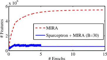
0 5 10 15
0 2 4 6x 10
6
# Epochs
# Features
MIRA
Sparceptron + MIRA (B=30)
Figure 2: Memory footprints of the MIRA and sparsep-tron algorithms in text chunking. The oscillation in the first 5 epochs (bottom line) comes from the proximal steps each K = 1000 rounds. The features are then frozen and 10 epochs of unregularized MIRA follow. Overall, the sparseptron requires<7.5%of the memory
as the MIRA baseline.
the model sizes obtained with the several budgets against those obtained by running 15 iterations of MIRA with the original set of features. Note that the total number of iterations is the same; yet, the group-Lasso approach has a much smaller memory footprint (see Fig. 2) and yields much more com-pact models. The small memory footprint comes from the fact that Alg. 1 may entertain a large num-ber of features without ever instantiating all of them. The predictive power is comparable (although some choices of budget yield slightly better scores for the group-Lasso approach).10
Named Entity Recognition. We experiment with the Spanish, Dutch, and English datasets pro-vided in the CoNLL 2002/2003 shared tasks (Sang, 2002; Sang and De Meulder, 2003). For Span-ish, we use the POS tags provided by
Car-(described next), we usedL2-regularized MIRA and tuned the
regularization constant with cross-validation.
10We also tried label-based Lasso and sparse group-Lasso (§3.1), with less impressive results (omitted for space).
reras (http://www.lsi.upc.es/˜nlp/tools/ nerc/nerc.html); for English, we ignore the
syn-tactic chunk tags provided with the dataset. Hence, all datasets have the same sort of input observations (words and POS) and all have9output labels. We use the feature templates described above plus some additional ones (yielding a total of452templates):
• Up to3-grams of shapes, in windows of size3; • For prefix/suffix sizes of1,2,3, up to3-grams of
word prefixes/suffixes, in windows of size3;
• Up to5-grams of case, punctuation, and digit in-dicators, in windows of size5.
As before, an additional feature template was de-fined to account for label bigrams. We do feature template selection (same setting as before) for bud-get sizes of 100, 200, and 300. We compare with both MIRA (using all the features) and the sparsep-tron with a standard Lasso regularizerΩL1
τ , for
2 4 6 8 10 12 x 106 76.5
77 77.5 78 78.5
Number of Features
UAS (%)
Arabic
0 5 10 15 x 106 89
89.2 89.4 89.6 89.8 90
Danish
0 2 4 6 8 x 10⁶ 92
92.5 93 93.5
Japanese
0 2 4 6 8 10 x 106 81
82 83 84
Slovene
0 0.5 1 1.5 2 x 10⁷ 82
82.5 83 83.5 84
Spanish
0 5 10 15 x 106 74
74.5 75 75.5 76
Turkish Group−Lasso
Group−Lasso (C2F) Lasso
[image:9.612.99.516.80.317.2]Filter−based (IG)
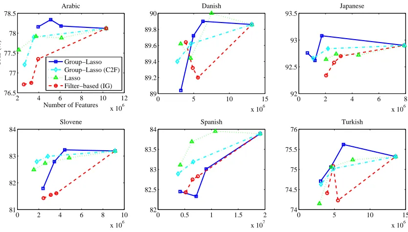
Figure 3: Comparison between non-overlapping group-Lasso, coarse-to-fine group-Lasso (C2F), and a filter-based method based on information gain for selecting feature templates in multilingual dependency parsing. Thex-axis is
the total number of features at different regularization levels, and they-axis is the unlabeled attachment score. The
plots illustrate how accurate the parsers are as a function of the model sparsity achieved, for each method. The standard Lasso (which does not select templates, but individual features) is also shown for comparison.
We use arc-factored models, for which exact infer-ence is tractable (McDonald et al., 2005). We de-fined M = 684 feature templates for each candi-date arc by conjoining the words, shapes, lemmas, and POS of the head and the modifier, as well as the contextual POS, and the distance and direction of attachment. We followed the same two-stage approach as before, and compared with a baseline which selects feature templates by ranking them ac-cording to the information gain criterion. This base-line assigns a score to each templateTm which
re-flects an empirical estimate of the mutual informa-tion betweenTmand the binary variableAthat
indi-cates the presence/absence of a dependency link:
IGm,
X
f∈Tm
X
a∈{0,1}
P(f, a) log2
P(f, a)
P(f)P(a), (16)
where P(f, a) is the joint probability of feature f firing and an arc being active (a = 1) or innactive (a = 0), andP(f)andP(a)are the corresponding marginals. All probabilities are estimated from the empirical counts of events observed in the data.
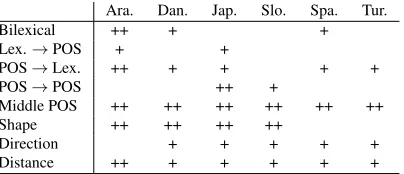
The results are plotted in Fig. 3, for budget sizes of 200, 300, and 400. We observe that for all but one language (Spanish is the exception), non-overlapping group-Lasso regularization is more ef-fective at selecting feature templates than the in-formation gain criterion, and slightly better than coarse-to-fine group-Lasso. For completeness, we also display the results obtained with a standard Lasso regularizer. Table 3 shows what kind of feature templates were most selected for each lan-guage. Some interesting patterns can be observed: morphologically-rich languages with small datasets (such as Turkish and Slovene) seem to avoid lexi-cal features, arguably due to potential for overfitting; in Japanese, contextual POS appear to be specially relevant. It should be noted, however, that some of these patterns may be properties of the datasets rather than of the languages themselves.
6 Related Work
Ara. Dan. Jap. Slo. Spa. Tur.
Bilexical ++ + +
Lex.→POS + +
POS→Lex. ++ + + + +
POS→POS ++ +
Middle POS ++ ++ ++ ++ ++ ++
Shape ++ ++ ++ ++
Direction + + + + +
[image:10.612.86.288.71.158.2]Distance ++ + + + + +
Table 3: Variation of feature templates that were selected accross languages. Each line groups together similar tem-plates, involving lexical, contextual POS, word shape in-formation, as well as attachment direction and length. Empty cells denote that very few or none of the templates in that category was selected; + denotes that some were selected; ++ denotes that most or all were selected.
(2011), along with a theoretical analysis. The fo-cus there, however, was multiple kernel learning, hence overlapping groups were not considered in their experiments. Budget-driven shrinkage and the sparseptron are novel techniques, at the best of our knowledge. Apart from Martins et al. (2011), the only work we are aware of which combines struc-tured sparsity with strucstruc-tured prediction is Schmidt and Murphy (2010); however, their goal is to pre-dict the structure of graphical models, while we are mostly interested in the structure of the feature space. Schmidt and Murphy (2010) used to gener-ative models, while our approach emphasizes dis-criminative learning.
Mixed norm regularization has been used for a while in statistics as a means to promote structured sparsity. Group Lasso is due to Bakin (1999) and Yuan and Lin (2006), after which a string of variants and algorithms appeared (Bach, 2008; Zhao et al., 2009; Jenatton et al., 2009; Friedman et al., 2010; Obozinski et al., 2010). The flat (non-overlapping) case has tight links with learning formalisms such as multiple kernel learning (Lanckriet et al., 2004) and multi-task learning (Caruana, 1997). The tree-structured case has been addressed by Kim and Xing (2010), Liu and Ye (2010) and Mairal et al. (2010), along with L∞,1 and L2,1 regularization.
Graph-structured groups are discussed in Jenatton et al. (2010), along with a DAG representation. In NLP, mixed norms have been used recently by Grac¸a et al. (2009) in posterior regularization, and by Eisenstein et al. (2011) in a multi-task regression problem.
7 Conclusions
In this paper, we have explored two levels of struc-ture in NLP problems: strucstruc-ture on the outputs, and structure on the feature space. We have shown how the latter can be useful in model design, through the use of regularizers which promote structured spar-sity. We propose an online algorithm with mini-mal memory requirements for exploring large fea-ture spaces. Our algorithm, which specializes into the sparseptron, yields a mechanism for selecting entire groups of features. We apply sparseptron for selecting feature templates in three structured prediction tasks, with advantages over filter-based methods,L1, andL2regularization in terms of
per-formance, compactness, and model interpretability.
Acknowledgments
We would like to thank all reviewers for their comments, Eric Xing for helpful discussions, and Slav Petrov for his comments on a draft version of this paper. A. M. was sup-ported by a FCT/ICTI grant through the CMU-Portugal Program, and also by Priberam. This work was partially supported by the FET programme (EU FP7), under the SIMBAD project (contract 213250). N. S. was supported by NSF CAREER IIS-1054319.
References
Y. Altun, I. Tsochantaridis, and T. Hofmann. 2003. Hid-den Markov support vector machines. In Proc. of ICML.
G. Andrew and J. Gao. 2007. Scalable training of L1-regularized log-linear models. InProc. of ICML. ACM.
F. Bach, R. Jenatton, J. Mairal, and G. Obozinski. 2011. Convex optimization with sparsity-inducing norms. In
Optimization for Machine Learning. MIT Press. F. Bach. 2008. Exploring large feature spaces with
hier-archical multiple kernel learning. NIPS, 21.
S. Bakin. 1999. Adaptive regression and model selec-tion in data mining problems. Ph.D. thesis, Australian National University.
S. Buchholz and E. Marsi. 2006. CoNLL-X shared task on multilingual dependency parsing. InProc. of CoNLL.
B. Carpenter. 2008. Lazy sparse stochastic gradient de-scent for regularized multinomial logistic regression. Technical report, Technical report, Alias-i.
S. F. Chen and R. Rosenfeld. 2000. A survey of smoothing techniques for maximum entropy models.
IEEE Transactions on Speech and Audio Processing, 8(1):37–50.
M. Collins. 2002a. Discriminative training methods for hidden Markov models: theory and experiments with perceptron algorithms. InProc. of EMNLP.
M. Collins. 2002b. Ranking algorithms for named-entity extraction: Boosting and the voted perceptron. In
Proc. of ACL.
K. Crammer, O. Dekel, J. Keshet, S. Shalev-Shwartz, and Y. Singer. 2006. Online Passive-Aggressive Algo-rithms. JMLR, 7:551–585.
S. Della Pietra, V. Della Pietra, and J. Lafferty. 1997. Inducing features of random fields. IEEE Transac-tions on Pattern Analysis and Machine Intelligence, 19:380–393.
J. Duchi and Y. Singer. 2009. Efficient online and batch learning using forward backward splitting. JMLR, 10:2873–2908.
J. Eisenstein, N. A. Smith, and E. P. Xing. 2011. Discov-ering sociolinguistic associations with structured spar-sity. InProc. of ACL.
M.A.T. Figueiredo. 2002. Adaptive sparseness using Jef-freys’ prior. Advances in Neural Information Process-ing Systems.
J. Friedman, T. Hastie, and R. Tibshirani. 2010. A note on the group lasso and a sparse group lasso. Unpub-lished manuscript.
J. Gao, G. Andrew, M. Johnson, and K. Toutanova. 2007. A comparative study of parameter estimation methods for statistical natural language processing. InProc. of ACL.
J. Goodman. 2004. Exponential priors for maximum en-tropy models. InProc. of NAACL.
J. Grac¸a, K. Ganchev, B. Taskar, and F. Pereira. 2009. Posterior vs. parameter sparsity in latent variable mod-els. Advances in Neural Information Processing Sys-tems.
I. Guyon and A. Elisseeff. 2003. An introduction to vari-able and feature selection. Journal of Machine Learn-ing Research, 3:1157–1182.
R. Jenatton, J.-Y. Audibert, and F. Bach. 2009. Struc-tured variable selection with sparsity-inducing norms. Technical report, arXiv:0904.3523.
R. Jenatton, J. Mairal, G. Obozinski, and F. Bach. 2010. Proximal methods for sparse hierarchical dictionary learning. InProc. of ICML.
J. Kazama and J. Tsujii. 2003. Evaluation and exten-sion of maximum entropy models with inequality con-straints. InProc. of EMNLP.
S. Kim and E.P. Xing. 2010. Tree-guided group lasso for multi-task regression with structured sparsity. InProc. of ICML.
J. Lafferty, A. McCallum, and F. Pereira. 2001. Con-ditional random fields: Probabilistic models for seg-menting and labeling sequence data. InProc. of ICML. G. R. G. Lanckriet, N. Cristianini, P. Bartlett, L. El Ghaoui, and M. I. Jordan. 2004. Learning the kernel matrix with semidefinite programming. JMLR, 5:27– 72.
J. Langford, L. Li, and T. Zhang. 2009. Sparse online learning via truncated gradient.JMLR, 10:777–801. T. Lavergne, O. Capp´e, and F. Yvon. 2010. Practical
very large scale CRFs. InProc. of ACL.
J. Liu and J. Ye. 2010. Moreau-Yosida regularization for grouped tree structure learning. InAdvances in Neural Information Processing Systems.
J. Mairal, R. Jenatton, G. Obozinski, and F. Bach. 2010. Network flow algorithms for structured sparsity. In
Advances in Neural Information Processing Systems. A. F. T. Martins, N. A. Smith, E. P. Xing, P. M. Q. Aguiar,
and M. A. T. Figueiredo. 2010. Turbo parsers: Depen-dency parsing by approximate variational inference. InProc. of EMNLP.
A. F. T. Martins, M. A. T. Figueiredo, P. M. Q. Aguiar, N. A. Smith, and E. P. Xing. 2011. Online learning of structured predictors with multiple kernels. InProc. of AISTATS.
A. McCallum. 2003. Efficiently inducing features of conditional random fields. InProc. of UAI.
R. T. McDonald, F. Pereira, K. Ribarov, and J. Hajic. 2005. Non-projective dependency parsing using span-ning tree algorithms. InProc. of HLT-EMNLP. G. Obozinski, B. Taskar, and M.I. Jordan. 2010. Joint
co-variate selection and joint subspace selection for multi-ple classification problems. Statistics and Computing, 20(2):231–252.
S. Petrov and D. Klein. 2008a. Discriminative log-linear grammars with latent variables. Advances in Neural Information Processing Systems, 20:1153–1160. S. Petrov and D. Klein. 2008b. Sparse multi-scale
gram-mars for discriminative latent variable parsing. In
Proc. of EMNLP.
A. Quattoni, X. Carreras, M. Collins, and T. Darrell. 2009. An efficient projection forl1,∞regularization.
InProc. of ICML.
E.F.T.K. Sang and S. Buchholz. 2000. Introduction to the CoNLL-2000 shared task: Chunking. InProceedings of CoNLL-2000 and LLL-2000.
E.F.T.K. Sang and F. De Meulder. 2003. Introduction to the CoNLL-2003 shared task: Language-independent named entity recognition. InProc. of CoNLL. E.F.T.K. Sang. 2002. Introduction to the
M. Schmidt and K. Murphy. 2010. Convex structure learning in log-linear models: Beyond pairwise poten-tials. InProc. of AISTATS.
S. Shalev-Shwartz, Y. Singer, and N. Srebro. 2007. Pe-gasos: Primal estimated sub-gradient solver for SVM. InICML.
N. Sokolovska, T. Lavergne, O. Capp´e, and F. Yvon. 2010. Efficient learning of sparse conditional random fields for supervised sequence labelling. IEEE Journal of Selected Topics in Signal Processing, 4(6):953–964. B. Taskar, C. Guestrin, and D. Koller. 2003. Max-margin Markov networks. InAdvances in Neural Information Processing Systems.
R. Tibshirani. 1996. Regression shrinkage and selection via the lasso. Journal of the Royal Statistical Society B., pages 267–288.
I. Tsochantaridis, T. Hofmann, T. Joachims, and Y. Altun. 2004. Support vector machine learning for interdepen-dent and structured output spaces. InICML.
Y. Tsuruoka, J. Tsujii, and S. Ananiadou. 2009. Stochas-tic gradient descent training for l1-regularized log-linear models with cumulative penalty. In Proc. of ACL.
S.J. Wright, R. Nowak, and M.A.T. Figueiredo. 2009. Sparse reconstruction by separable approximation.
IEEE Transactions on Signal Processing, 57(7):2479– 2493.
L. Xiao. 2009. Dual averaging methods for regular-ized stochastic learning and online optimization. In
Advances in Neural Information Processing Systems. M. Yuan and Y. Lin. 2006. Model selection and
estima-tion in regression with grouped variables. Journal of the Royal Statistical Society (B), 68(1):49.
P. Zhao, G. Rocha, and B. Yu. 2009. Grouped and hi-erarchical model selection through composite absolute penalties. Annals of Statistics, 37(6A):3468–3497. H. Zou and T. Hastie. 2005. Regularization and