A causal framework for explaining the predictions of
black-box sequence-to-sequence models
David Alvarez-Melis and Tommi S. Jaakkola CSAIL, MIT
{davidam, tommi}@csail.mit.edu
Abstract
We interpret the predictions of any black-box structured input-structured output model around a specific input-output pair. Our method returns an “explanation” con-sisting of groups of input-output tokens that are causally related. These dependen-cies are inferred by querying the black-box model with perturbed inputs, generating a graph over tokens from the responses, and solving a partitioning problem to se-lect the most relevant components. We fo-cus the general approach on sequence-to-sequence problems, adopting a variational autoencoder to yield meaningful input per-turbations. We test our method across sev-eral NLP sequence generation tasks.
1 Introduction
Interpretability is often the first casualty when adopting complex predictors. This is particularly true for structured prediction methods at the core of many natural language processing tasks such as machine translation (MT). For example, deep learning models for NLP involve a large num-ber of parameters and complex architectures, mak-ing them practically black-box systems. While such systems achieve state-of-the-art results in MT (Bahdanau et al.,2014), summarization (Rush et al., 2015) and speech recognition (Chan et al.,
2015), they remain largely uninterpretable, al-though attention mechanisms (Bahdanau et al.,
2014) can shed some light on how they operate.
Stronger forms of interpretability could offer several advantages, from trust in model
predic-tions, error analysis, to model refinement. For example, critical medical decisions are increas-ingly being assisted by complex predictions that should lend themselves to easy verification by hu-man experts. Without understanding how inputs get mapped to the outputs, it is also challenging to diagnose the source of potential errors. A slightly less obvious application concerns model improve-ment (Ribeiro et al., 2016) where interpretability can be used to detect biases in the methods.
Interpretability has been approached primarily from two main angles:model interpretability, i.e., making the architecture itself interpretable, and
prediction interpretability, i.e., explaining particu-lar predictions of the model (cf. (Lei et al.,2016)). Requiring the model itself to be transparent is of-ten too restrictive and challenging to achieve. In-deed, prediction interpretability can be more eas-ily soughta posteriori for black-box systems in-cluding neural networks.
In this work, we propose a novel approach to prediction interpretability with only oracle access to the model generating the prediction. Following (Ribeiro et al., 2016), we turn the local behavior of the model around the given input into an inter-pretable representation of its operation. In con-trast to previous approaches, we consider struc-tured prediction where both inputs and outputs are combinatorial objects, and our explanation con-sists of a summary of operation rather than a sim-pler prediction method.
Our method returns an “explanation” consisting of sets of input and output tokens that are causally related under the black-box model. Causal de-pendencies arise from analyzing perturbed ver-sions of inputs that are passed through the
box model. Although such perturbations might be available in limited cases, we generate them auto-matically. For sentences, we adopt a variational autoencoder to produce semantically related sen-tence variations. The resulting inferred causal de-pendencies (interval estimates) form a dense bi-partite graph over tokens from which explanations can be derived as robust min-cut k-partitions.
We demonstrate quantitatively that our method can recover known dependencies. As a starting point, we show that a grapheme-to-phoneme dic-tionary can be largely recovered if given to the method as a black-box model. We then show that the explanations provided by our method closely resemble the attention scores used by a neural ma-chine translation system. Moreover, we illustrate how our summaries can be used to gain insights and detect biases in translation systems. Our main contributions are:
• We propose a general framework for explain-ing structured black-box models
• For sequential data, we propose a variational autoencoder for controlled generation of in-put perturbations required for causal analysis
• We evaluate the explanations produced by our framework on various sequence-to-sequence prediction tasks, showing they can recover known associations and provide in-sights into the workings of complex systems.
2 Related Work
There is a wide body of work spanning vari-ous fields centered around the notion of “inter-pretability”. This term, however, is underdeter-mined, so the goals, methods and formalisms of these approaches are often non-overlapping ( Lip-ton, 2016). In the context of machine learning, perhaps the most visible line of work on inter-pretability focuses on medical applications ( Caru-ana et al., 2015), where trust can be a decisive factor on whether a model is used or not. With the ever-growing success and popularity of deep learning methods for image processing, recent work has addressed interpretability in this setting, usually requiring access to the method’s activa-tions and gradients (Selvaraju et al.,2016), or di-rectly modeling how influence propagates (Bach
et al.,2015). For a broad overview of interpretabil-ity in machine learning, we refer the reader to the recent survey byDoshi-Velez and Kim(2017).
Most similar to this work are the approaches of
Lei et al.(2016) andRibeiro et al.(2016). The for-mer proposes a model that justifies its predictions in terms of fragments of the input. This approach formulates explanation generation as part of the learning problem, and, as most previous work, only deals with the case where predictions are scalar or categorical. On the other hand,Ribeiro et al.(2016) propose a framework for explaining the predictions of black-box classifiers by means of locally-faithful interpretable models. They fo-cus on sparse linear models as explanations, and rely on local perturbations of the instance to ex-plain. Their model assumes the input directly ad-mits a fixed size interpretable representation in eu-clidean space, so their framework operates directly on this vector-valued representation.
Our method differs from—and can be thought of as generalizing—these approaches in two fun-damental aspects. First, our framework considers both inputs and outputs to be structured objects thus extending beyond the classification setting. This requires rethinking the notion of explanation to adapt it to variable-size combinatorial objects. Second, while our approach shares the locality and model-agnostic view ofRibeiro et al.(2016), gen-erating perturbed versions of structured objects is a challenging task by itself. We propose a solu-tion to this problem in the case of sequence-to-sequence learning.
3 Interpreting structured prediction
decomposes an explanation into (potentially sev-eral)explaining components, each of which justi-fies, from the perspective of the black-box model, parts of the output relative to the parts of the input.
Formally, suppose we have a black-box model
F : X → Y that maps a structured inputx ∈ X
to a structured output y ∈ Y. We make no as-sumptions on the spaces X,Y, except that their elements admit a feature-set representation x =
{x1, x2, . . . , xn},y ={y1, y2, . . . , ym}. Thus,x
and y can be sequences, graphs or images. We refer to the elements xi and yj as units or
“to-kens” due to our motivating application of sen-tences, though everything in this work holds for other combinatorial objects.
For a given input output pair(x,y), we are in-terested in obtaining anexplanationofyin terms of x. Following (Ribeiro et al., 2016), we seek explanations viainterpretable representationsthat are both i) locally faithful, in the sense that they approximate how the model behaves in the vicinity ofx, and ii)model agnostic, that is, that do not re-quire any knowledge ofF. For example, we would like to identify whether tokenxi is a likely cause
for the occurrence ofyjin the output when the
in-put context is x. Our assumption is that we can summarize the behavior of F around x in terms of a weighted bipartite graphG = (Vx∪Vy, E),
where the nodesVx andVy correspond to the
el-ements in x and y, respectively, and the weight of each edgeEij corresponds to the influence of
the occurrence of tokenxi on the appearance of
yj. The bipartite graph representation suggests
naturally that the explanation be given in terms of explaining components. We can formalize these components as subgraphs Gk = (Vk
x ∪Vyk, Ek),
where the elements in Vk
x are likely causes for
the elements in Vk
y . Thus, we define an
expla-nation of y as a collection of such components:
Ex→y ={G1, . . . , Gk}.
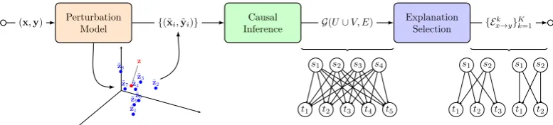
Our approach formalizes this framework through a pipeline (sketched in Figure1) consist-ing of three main components, described in detail in the following section: a perturbation model for exercising F locally, a causal inference model for inferring associations between inputs and pre-dictions, and a selection step for partitioning and selecting the most relevant sets of associations.
We refer to this framework as astructured-output causal rationalizer(SOCRAT).
A note on alignment models When the inputs and outputs are sequences such as sentences, one might envision using an alignment model, such as those used in MT, to provide an explanation. This differs from our approach in several respects. Specifically, we focus on explaining the behavior of the “black box” mappingFonly locally, around the current input context, not globally. Any global alignment model would require access to substan-tial parallel data to train and would have vary-ing coverage of the local context around the spe-cific example of interest. Any global model would likely also suffer from misspecification in relation toF. A more related approach to ours would be an alignment model trained locally based on the same perturbed sentences and associated outputs that we generate.
4 Building blocks
4.1 Perturbation Model
The first step in our approach consists of obtain-ingperturbedversions of the input: semantically similar to the original but with potential changes in elements and their order. This is a major challenge with any structured inputs. We propose to do this using a variational autoencoder (VAE) (Kingma and Welling,2014;Rezende et al., 2014). VAEs have been successfully used with fixed dimen-sional inputs such as images (Rezende and Mo-hamed,2015;Sønderby et al.,2016) and recently also adapted to generating sentences from contin-uous representations (Bowman et al.,2016). The goal is to introduce the perturbation in the contin-uous latent representation rather than directly on the structured inputs.
A VAE is composed of a probabilistic encoder ENC : X → Rd and a decoder DEC : Rd →
Perturbation
Model InferenceCausal ExplanationSelection
(x,y) {(˜xi,y˜i)} G(U∪V, E) {Exk→y}Kk=1
z
˜
z1
˜
z2
˜
z3
˜
z4
˜
z5˜z6
˜
z7
˜
z8 s1 s2 s3 s4
t1 t2 t3 t4 t5
s1 s2
t1 t2 t3 s1 s2
[image:4.595.104.493.61.149.2]t1 t2
Figure 1: A schematic representation of the proposed prediction interpretability method.
by sampling repeatedly from this distribution, and then mapping these back to the original space us-ing the decoder. The trainus-ing regime for the VAE ensures approximately that a small perturbation of the hidden representation maintains similar se-mantic content while introducing small changes in the decoded surface form. We emphasize that the approach would likely fail with an ordinary au-toencoder where small changes in the latent rep-resentation can result in large changes in the de-coded output. In practice, we ensure diversity of perturbations by scaling the variance term σ and sampling points ˜z and different resolutions. We provide further details of this procedure in the sup-plement. Naturally, we can train this perturba-tion model in advance on (unlabeled) data from the input domain X, and then use it as a subrou-tine in our method. After this process is com-plete, we have N pairs of perturbed input-output pairs: {(˜xi,y˜i)}Ni=1 which exercise the mapping F around semantically similar inputs.
4.2 Causal model
The second step consists of using the perturbed input-output pairs{(˜xi,y˜i)}Ni=1to infer causal
de-pendencies between the original input and output tokens. A naive approach would consider 2x2 con-tingency tables representing presence/absence of input/output tokens together with a test statistic for assessing their dependence. Instead, we incorpo-rateallinput tokens simultaneously to predict the occurrence of a single output token via logistic re-gression. The quality of these dependency estima-tors will depend on the frequency with which each input and output token occurs in the perturbations. Thus, we are interested in obtaining uncertainty estimates for these predictions, which can be nat-urally done with a Bayesian approach to logistic regression. Letφx(˜x)∈ {0,1}|x|be a binary
vec-tor encoding the presence of the original tokens
x1, . . . , xnfromxin the perturbed versionx˜. For
each target tokenyj ∈y, we estimate a model:
P(yj ∈y˜|x˜) =σ(θjTφx(˜x)) (1)
whereσ(z) = (1 + exp(−z))−1. We use a
Gaus-sian approximation for the logarithm of the lo-gistic function together with the prior p(θ) =
N(θ0,H−01)(Murphy,2012). Since in our case all
tokens are guaranteed to occur at least once (we in-clude the original example pair as part of the set), we useθ0 =α1,H0 =βI, withα, β >0. Upon
completion of this step, we have dependency co-efficients between all original input and output to-kens{θij}, along with their uncertainty estimates.
4.3 Explanation Selection
The last step in our interpretability framework consists of selecting a set explanations for(x,y). The steps so far yield a dense bipartite graph be-tween the input and output tokens. Unless|x|and
|y| are small, this graph itself may not be suf-ficiently interpretable. We are interested in se-lecting relevant components of this dependency graph, i.e., partition the vertex set of G into dis-joint subsets so as to minimize the weight of omit-ted edges (i.e. the k-cut value of the partition).
Algorithm 1Structured-output causal rationalizer
1: procedureSOCRAT(x,y, F)
2: (µ,σ)←ENCODE(x)
3: fori= 1toNdo
4: ˜zi←SAMPLE(µ,σ)
Perturbation Model. 5: x˜i←DECODE(˜zi)
6: y˜i←F(˜xi)
7: end for
8: G ←CAUSAL(x,y,{˜xi,y˜i}Ni=1)
9: Ex7→y←BIPARTITION(G)
10: Ex7→y←SORT(Ex7→y) .By cut capacity
11: returnEx7→y
12: end procedure
with edge weights given as uncertainty intervals
θij±θˆij, the partitioning problem is given by
min (xu
ik,xvjk,yij)∈Y n
X
i=1
m
X
j=1
θijyij+
max
S:S⊆V,|S|≤Γ
(it,jt)∈V\S
X
(i,j)∈S
ˆ
θijyij+ (Γ− bΓc)ˆθit,jtyit,jt
(2) wherexu
ik,xvjkare binary variables indicating
sub-set belonging for elements of U and V respec-tively,yij are binary auxiliary variables indicating
whetheriandj are in different partitions, andY
is a set of constraints that ensure the K-partition is valid. Γis a parameter in[0,|V|]which adjusts the robustness of the partition (the number of de-viations from the mean edge values). See the sup-plement for further explanation of this objective.
If |x| and |y| are small, the number of clus-ters K will also be small, so we can simply re-turn all the partitions (i.e. theexplanation chunks)
Ek
x→y := (Vxk∪Vyk). However, whenK is large,
one might wish to entertain only theκ most rele-vant explanations. The graph partitioning frame-work provides us with a natural way to score the importance of each chunk. Intuitively, subgraphs that have few high-valued edges connecting them to other parts of the graph (i.e. lowcut-capacity) can be thought of asself-contained explanations, and thus more relevant for interpretability. We can therefore define the importance score an atom as:
importance(Exk→y) :=− X
(i,j)∈Xk
θij (3)
whereXkis the cut-set implied byExk→y:
Xk={(i, j)∈E|i∈Exk→y, j∈V \Exk→y}
The full interpretability method is succinctly ex-pressed in Algorithm1.
5 Experimental Framework
5.1 Training and optimization
For the experiments involving sentence inputs, we train in advance the VAE described in Section4.1. We use symmetric encoder-decoders consisting of recurrent neural networks with an intermediate variational layer. In our case, however, we useL
stacked RNN’s on both sides, and a stacked varia-tional layer. Training variavaria-tional autoencoders for text is notoriously hard. In addition to dropout and KLD annealing (Bowman et al., 2016), we found that slowly scaling the variance sampled from the normal distribution from 0 to 1 made training much more stable.
For the partitioning step we compare the robust formulation described above with two classical ap-proaches to bipartite graph partitioning which do not take uncertainty into account: the cocluster-ing method of Dhillon (2001) and the bicluster-ing method ofKluger et al.(2003). For these two, we use off-the-shelf implementations,1 while we solve the MIP problem version of (2) with the op-timization librarygurobi.2
5.2 Recovering simple mappings
Before using our interpretability framework in real tasks where quantitative evaluation of explana-tions is challenging, we test it in a simplified set-ting where the “black-box” is simple and fully known. A reasonable minimum expectation on our method is that it should be able to infer many of these simple dependencies. For this purpose, we use the CMU Dictionary of word pronunci-ations,3 which is based on the ARPAbet symbol set and consists of about 130K word-to-phoneme pairs. Phonemes are expressed as tokens of 1 to 3 characters. An example entry in this dictio-nary is the pair vowels 7→ V AW1 AH0 L Z. Though the mapping is simple, it is not one-to-one (a group of characters can correspond to a sin-gle phoneme) nor deterministic (the same charac-ter can map to different phonemes depending on the context). Thus, it provides a reasonable testbed 1http://scikit-learn.org/stable/modules/biclustering.html 2http://www.gurobi.com/
20 40 60 80 100
Samples
0.50 0.55 0.60 0.65 0.70 0.75 0.80 0.85
AER
Align - Full Vocab
20 40 60 80 100
Samples
0.3 0.4 0.5 0.6 0.7 0.8 0.9 1.0
F1
Align - Full Vocab
[image:6.595.305.521.61.181.2]Uncertainty Biclustering Coclustering Alignment
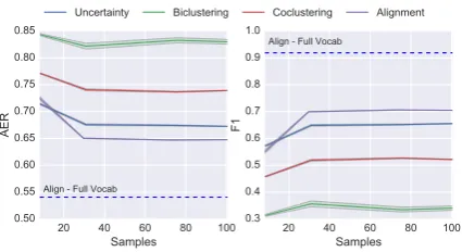
Figure 2: Arpabet test results as a function of num-ber of perturbations used. Shown are mean plus confidence bounds over 5 repetitions.Left: Align-ment Error Rate,Right: F1 over edge prediction.
for our method. The setting is as follows: given an input-output pair from thecmudict“black-box”, we use our method to infer dependencies between characters in the input and phonemes in the out-put. Since locality in this context is morphologi-cal instead of semantic, we produce perturbations selectingnwords randomly from the intersection of thecmudictvocabulary and the set of words with edit distance at most 2 from the original word.
To evaluate the inferred dependencies, we ran-domly selected 100 key-value pairs from the dic-tionary and manually labeled them with character-to-phoneme alignments. Even though our frame-work is not geared to produce pairwise align-ments, it should nevertheless be able to recover them to a certain extent. To provide a point of reference, we compare against a (strong) base-line that is tailored to such a task: a state-of-the-art unsupervised word alignment method based on Monte Carlo inference (Tiedemann and Östling,
2016). The results in Figure 2 show that the version of our method that uses the uncertainty clustering performs remarkably close to the align-ment system, with an alignalign-ment error rate only ten points above an oracle version of this system that was trained on thefullarpabet dictionary (dashed line). The raw and partitioned explanations pro-vided by our method for an example input-output pair are shown in Table1, where the edge widths correspond to the estimated strength of depen-dency. Throughout this work we display the nodes in the same lexical order of the inputs/outputs to facilitate reading, even if that makes the explana-tion chunks less visibly discernible. Instead, we sometimes provide an additional (sorted) heatplot
Raw Dependencies Explanation Graph
o
b o a n
UW0
l e
IY1 AH0
B L N
→
o
b o a n
UW0
l e
IY1 AH0
B L N
o
b o a n
UW0
l e
IY1 AH0
B L N
→
o
b o a n
UW0
l e
IY1 AH0
[image:6.595.75.288.65.181.2]B L N
Table 1: Inferred dependency graphs before (left) and after (right) explanation selection for the pre-diction: boolean7→ B UW0 L IY1 AH0 N, in independent runs with large (top) and small (bot-tom) clustering parameterk.
of dependency values to show these partitions.
5.3 Machine Translation
In our second set of experiments we evaluate our explanation model in a relevant and popular sequence-to-sequence task: machine translation. As black-boxes, we use three different methods for translating English into German: (i) Azure’s Ma-chine Translation system, (ii) a Neural MT model, and (iii) a human (native speaker of German). We provide details on all three systems in the supple-ment. We translate the same English sentences with all three methods, and explain their predic-tions using SOCRAT. To be able to generate sen-tences with similar language and structure as those used to train the two automatic systems, we use the monolingual English side of the WMT14 dataset to train the variational autoencoder described in Section 4.1. For every explanation instance, we sampleS = 100perturbations and use the black-boxes to translate them. In all cases, we use the same default SOCRAT configurations, including the robust partitioning method.
Studenten sagten, dass sie nach vorne
Klasse aussah. in seine . his to class forward looked they said Students class sagten, looked dass forward they said
vorne in Klasse
sie seine to aussah. nach Studenten . Students his Studenten sagten , sie dass auf freuen . seine Klasse class his . to forward looked they said Students class sagten looked , forward they said
auf seine freuen
[image:7.595.309.521.63.259.2]dass Klasse to . sie Studenten . Students his Studenten sagten sie würden seiner Vorlesung entgegensehen. . class his to forward looked they said Students class sagten looked sie forward they said Vorlesung . entgegensehen. würden to seiner Studenten Students his
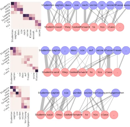
Figure 3: Explanations for the predictions of three Black-Box translators: Azure (top), NMT (mid-dle) and human (bottom). Note that the rows and columns of the heatmaps are permuted to show ex-planationchunks(clusters).
dependency coefficients are overall higher for the human than for the other systems, suggesting more coherence in the translations (potentially because the human translated sentences in context, while the two automatic systems carry over no informa-tion from one example to the next).
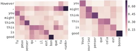
The NMT system, as opposed to the other two, is not truly a black-box. We can open the boxto get a glimpse on the true dependencies on the in-puts used by the system at prediction time (the at-tention weights) and compare them to the expla-nation graph. The attention matrix, however, is dense and not normalized over target tokens, so it is not directly comparable to our dependency scores. Nevertheless, we can partition it with the coclustering method described in Section 4.3 to enforce group structure and make it easier to com-pare. Figure4shows the attention matrix and the explanation for an example sentence of the test set. Their overall cluster structure agrees, though our method shows conservatism with respect to the dependencies of the function words (to, for). In-terestingly, our method is able to figure out that
the<unk>token was likely produced by the word
“appeals”, as shown by the explanation graph.
It must be emphasized that although we
dis-Dies würde <unk>
. gegen ermöglichen Urteile judgements againstmade be to. appealsfor allow would This
Dies würde <unk>
. gegen ermöglichen Urteile 0.00 0.15 0.30 0.45 0.60
Dies würde <unk>
ermöglichen Urteile gegen . . against made to judgements be for appeals allow would This made würde for <unk> appeals allow would ermöglichen against . gegen to judgements Urteile Dies
This be .
Figure 4: Top: Original and clustered attention matrix of the NMT system for a given translation. Bottom: Dependency estimates and explanation graph generated by SOCRATwith withS= 100.
play attention scores in various experiments in this work, we do so only for qualitative evaluation pur-poses. Our model-agnostic framework can be used on top of models that do not use attention mech-anisms or for which this information is hard to extract. Even in cases where it is available, the explanation provided by SOCRATmight be com-plementary or even preferable to attention scores because: (a) being normalized on both directions (as opposed to only over source tokens) and parti-tioned, it is often more interpretable than a dense attention matrix, and (b) it can be retrievedchunk -by-chunkin decreasing order of relevance, which is especially important when explaining large in-puts and/or outin-puts.
5.4 A (mediocre) dialogue system
[image:7.595.73.292.66.280.2]Input Prediction
[image:8.595.312.525.62.122.2]What do you mean it doesn’t matter? I don’t know Perhaps have we met before? I don’t think so Can I get you two a cocktail? No, thanks.
Table 2: “Good” dialogue system predictions.
don't
it know.
What do I
doesn't matter? mean
you
I
don't know.
? matter t ' doesn it mean you do What
0.15 0.30 0.45 0.60 0.75
Figure 5: Explanation withS = 50 (left) and at-tention (right) for the first prediction in Table2.
Although most of the predictions of this model are short and repetitive (Yes/No/<unk>answers), some of them are seemingly meaningful, and might—if observed in isolation—lead one to be-lieve the system is much better than it actually is. For example, the predictions in Table2suggest a complex use of the input to generate the output. To better understand this model, we rationalize its predictions using SOCRAT. The explanation graph for one such “good” prediction, shown in Figure5, suggests that there is little influence of anything except the tokensWhat and youon the output. Thus, our method suggests that this model is using only partial information of the input and has probably memorized the connection between question words and responses. This is confirmed upon inspecting the model’s attention scores for this prediction (same figure, right pane).
5.5 Bias detection in parallel corpora
Natural language processing methods that derive semantics from large corpora have been shown to incorporate biases present in the data, such as archaic stereotypes of male/female occupations (Caliskan et al., 2017) and sexist adjective asso-ciations (Bolukbasi et al., 2016). Thus, there is interest in methods that can detect and address those biases. For our last set of experiments, we use our approach to diagnose and explain biased translations of MT systems, first on a simplistic but verifiable synthetic setting, where we inject
is il
you
penser bon que
think est
good peux
However, might
Tu qu
this
[image:8.595.78.287.160.256.2]<unk> tu
Figure 6: Explanation withS= 50for the predic-tion of the biased translator.
Tu
peux
penser
qu il est bon que tu
<unk>
good is this think might you , However
Vous
pourriez penser que cela est
bonne
good is this think might you
0.15 0.30 0.45 0.60
Figure 7: Attention scores on similar sentences by the biased translator.
a pre-specified spurious association into an other-wise normal parallel training corpus, and then on an industrial-quality black-box system.
[image:8.595.306.531.172.257.2]very est
dancer
charmante
This Cette
charming is
danseuse très
very est
doctor
talentueux
This Ce
talented is
médecin très personnes sont
These are
Ces très
people
bizarres
[image:9.595.81.516.63.134.2]odd very
Figure 8: Explanations for biased translations of similar gender-neutral English sentences into French generated with Azure’s MT service. The first two require gender declination in the target (French) language, while the third one, in plural, does not. The dependencies in the first two shed light on the cause of the biased selection of gender in the output sentence.
results in a switch to the formal register, as shown in the second plot in Figure7.
Although somewhat contrived, this synthetic setting works as a litmus test to show that our method is able to detect known artificial biases from a model’s predictions. We now move to a real setting, where we investigate biases in the predictions of an industrial-quality translation sys-tem. We use Azure’s MT service to translate into French various simple sentences that lack gender specification in English, but which require gender-declined words in the output. We choose sentences containing occupations and adjectives previously shown to exhibit gender biases in linguistic cor-pora (Bolukbasi et al.,2016). After observing the choice of gender in the translation, we use SO -CRATto explain the output.
In line with previous results, we observe that this translation model exhibits a concerning pref-erence for the masculine grammatical gender in sentences containing occupations such asdoctor, professor or adjectives such as smart, talented, while choosing the feminine gender for charm-ing, compassionate subjects who are dancers or
nurses. The explanation graphs for two such examples, shown in Figure 8 (left and center), suggest strong associations between the gender-neutral but stereotype-prone source tokens (nurse, doctor, charming) and the gender-carrying target tokens (i.e. the feminine-declinedcette, danseuse, charmante in the first sentence and the mascu-linece, médecin, talenteuxin the second). While it is not unusual to observe interactions between multiple source and target tokens, the strength of dependence in some of these pairs ( charm-ing→danseuse, doctor→ce) is unexplained from a grammatical point of view. For comparison, the third example—a sentence in the plural form that
does not involve choice of grammatical gender in French—shows comparatively much weaker asso-ciations across words in different parts of the sen-tence.
6 Discussion
Our model-agnostic framework for prediction in-terpretability with structured data can produce rea-sonable, coherent, and often insightful explana-tions. The results on the machine translation task demonstrate how such a method yields a partial view into the inner workings of a black-box sys-tem. Lastly, the results of the last two exper-iments also suggest potential for improving ex-isting systems, by questioning seemingly correct predictions and explaining those that are not.
The method admits several possible modifi-cations. Although we focused on sequence-to-sequence tasks, SOCRATgeneralizes to other set-tings where inputs and outputs can be expressed as sets of features. An interesting application would be to infer dependencies between textual and age features in image-to-text prediction (e.g. im-age captioning). Also, we used a VAE-based sam-pling for object perturbations but other approaches are possible depending on the nature of the domain or data.
Acknowledgments
References
Sebastian Bach, Alexander Binder, Grégoire Mon-tavon, Frederick Klauschen, Klaus-Robert Müller, and Wojciech Samek. 2015. On Pixel-Wise Ex-planations for Non-Linear Classifier Decisions by Layer-Wise Relevance Propagation. PLoS One, 10(7):1–46.
Dzmitry Bahdanau, Kyunghyun Cho, and Yoshua Ben-gio. 2014. Neural Machine Translation By Jointly Learning To Align and Translate. Iclr 2015, pages 1–15.
Tolga Bolukbasi, Kai-Wei Chang, James Zou, Venkatesh Saligrama, and Adam Kalai. 2016. Man is to Computer Programmer as Woman is to Home-maker? Debiasing Word Embeddings. NIPS, (Nips):4349—-4357.
Samuel R. Bowman, Luke Vilnis, Oriol Vinyals, An-drew M. Dai, Rafal Jozefowicz, and Samy Ben-gio. 2016. Generating Sentences from a Continuous Space.Iclr, pages 1–13.
Aylin Caliskan, Joanna J Bryson, and Arvind Narayanan. 2017. Semantics derived automatically from language corpora contain human-like biases.
Science (80-. )., 356(6334):183–186.
Rich Caruana, Yin Lou, Johannes Gehrke, Paul Koch, Marc Sturm, and Noemie Elhadad. 2015. Intelligi-ble Models for HealthCare : Predicting Pneumonia Risk and Hospital 30-day Readmission. Proc. 21th ACM SIGKDD Int. Conf. Knowl. Discov. Data Min. - KDD ’15, pages 1721–1730.
William Chan, Navdeep Jaitly, Quoc V. Le, and Oriol Vinyals. 2015. Listen, attend and spell. arXiv Prepr., pages 1–16.
Inderjit s. Dhillon. 2001. Co-clustering documents and words using Bipartite spectral graph partition-ing.Proc 7th ACM SIGKDD Conf, pages 269–274.
Finale Doshi-Velez and Been Kim. 2017. A Roadmap for a Rigorous Science of Interpretability. ArXiv e-prints, (Ml):1–12.
Neng Fan, Qipeng P. Zheng, and Panos M. Pardalos. 2012. Robust optimization of graph partitioning in-volving interval uncertainty. InTheor. Comput. Sci., volume 447, pages 53–61.
M. R. Garey, D. S. Johnson, and L. Stockmeyer. 1976. Some simplified NP-complete graph prob-lems.Theor. Comput. Sci., 1(3):237–267.
Diederik P Kingma and Max Welling. 2014. Auto-Encoding Variational Bayes.Iclr, (Ml):1–14.
G. Klein, Y. Kim, Y. Deng, J. Senellert, and A. M. Rush. 2017. OpenNMT: Open-Source Toolkit for Neural Machine Translation.ArXiv e-prints.
Yuval Kluger, Ronen Basri, Joseph T. Chang, and Mark Gerstein. 2003. Spectral biclustering of microarray data: Coclustering genes and conditions.
Tao Lei, Regina Barzilay, and Tommi Jaakkola. 2016.
Rationalizing Neural Predictions. InEMNLP 2016, Proc. 2016 Conf. Empir. Methods Nat. Lang. Pro-cess., pages 107–117.
Zachary C Lipton. 2016. The Mythos of Model In-terpretability. ICML Work. Hum. Interpret. Mach. Learn., (Whi).
Kevin P. Murphy. 2012. Machine Learning: A Proba-bilistic Perspective.
D J Rezende, S Mohamed, and D Wierstra. 2014.
Stochastic backpropagation and approximate infer-ence in deep generative models. Proc. 31st . . ., 32:1278–1286.
Danilo Jimenez Rezende and Shakir Mohamed. 2015.
Variational Inference with Normalizing Flows.
Proc. 32nd Int. Conf. Mach. Learn., 37:1530–1538. Marco Tulio Ribeiro, Sameer Singh, and Carlos Guestrin. 2016. "Why Should I Trust You?": Ex-plaining the Predictions of Any Classifier. InProc. 22Nd ACM SIGKDD Int. Conf. Knowl. Discov. Data Min., KDD ’16, pages 1135–1144, New York, NY, USA. ACM.
Alexander M Rush, Sumit Chopra, and Jason Weston. 2015. A Neural Attention Model for Abstractive Sentence Summarization. Proc. Conf. Empir. Meth-ods Nat. Lang. Process., (September):379–389. Ramprasaath R. Selvaraju, Abhishek Das,
Ramakr-ishna Vedantam, Michael Cogswell, Devi Parikh, and Dhruv Batra. 2016. Grad-CAM: Why did you say that? Visual Explanations from Deep Networks via Gradient-based Localization. (Nips):1–5. Casper Kaae Sønderby, Tapani Raiko, Lars Maaløe,
Søren Kaae Sønderby, and Ole Winther. 2016. Lad-der Variational AutoencoLad-ders.NIPS, (Nips). Jörg Tiedemann. 2009. News from OPUS - A
Collec-tion of Multilingual Parallel Corpora with Tools and Interfaces. In N. Nicolov, G. Bontcheva, G. An-gelova, and R. Mitkov, editors, Recent Adv. Nat. Lang. Process., pages 237—-248. John Benjamins, Amsterdam/Philadelphia.
Jörg Tiedemann and Robert Östling. 2016. Efficient Word Alignment with Markov Chain Monte Carlo.