Statistical approaches to the study of protein folding and energetics

(1)

University of Warwick institutional repository: http://go.warwick.ac.uk/wrap

A Thesis Submitted for the Degree of PhD at the University of Warwick

http://go.warwick.ac.uk/wrap/66470

This thesis is made available online and is protected by original copyright.

Please scroll down to view the document itself.

(2)

Statistical approaches to the study of

protein folding and energetics

by

Nikolas S. Burkoff

Thesis

Submitted to the University of Warwick

for the degree of

Doctor of Philosophy

MOAC Doctoral Training Centre

(3)

(4)

Acknowledgements

I would like thank my supervisor, Professor David Wild, for his support and insights throughout the project. I would also like to take this opportunity to thank collaborators I have worked with over the last few years: Dr. G´abor Cs´anyi and Robert Baldock for their work developing the molecular dynamics nested sampling algorithm, Dr. Stephen Wells for his work with rigidity analysis and Dr. John Skilling for general nested sampling and maximum entropy discussions.

I thank the staff of both WSB and MOAC for helping the project run smoothly, particularly Dr. Paul Brown and Sam Mason for their computational support. I would also like to acknowledge the Leverhulme Trust for providing the funding throughout my PhD. Finally, I would like to thank Dr. Csilla V´arnai for her hard work and helpful discussions over the last three years and for her calming influence, helping me to continue when the project was going through tough patches. Thank you.

(7)

(8)

Declarations

This thesis is submitted to the University of Warwick in support of my application for the degree of Doctor of Philosophy. Unless explicitly stated otherwise, all parts have been composed by myself and have not been submitted in any previous application for any degree. The novel work in this thesis is presented in journal paper format and prefacing each paper there is a summary of my contribution to the work.

(9)

(10)

Abstract

The determination of protein structure and the exploration of protein folding landscapes are two of the key problems in computational biology. In order to address these challenges, both a protein model that accurately captures the physics of interest and an efficient sampling algorithm are required.

The first part of this thesis documents the continued development of CRANKITE, a coarse-grained protein model, and its energy landscape exploration using nested sampling, a Bayesian sampling algo-rithm.

We extend CRANKITE and optimize its parameters using a maximum likelihood approach. The efficiency of our procedure, using the contrastive divergence approximation, allows a large training set to be used, producing a model which is transferable to proteins not included in the training set.

We develop an empirical Bayes model for the prediction of protein β-contacts, which are required inputs for CRANKITE. Our approach couples the constraints and prior knowledge associated with β -contacts to a maximum entropy-based statistic which predicts evolutionarily-related -contacts.

Nested sampling (NS) is a Bayesian algorithm shown to be efficient at sampling systems which exhibit a first-order phase transition. In this work we parallelize the algorithm and, for the first time, apply it to a biophysical system: small globular proteins modelled using CRANKITE. We generate energy landscape charts, which give a large-scale visualization of the protein folding landscape, and we compare the efficiency of NS to an alternative sampling technique, parallel tempering, when calculating the heat capacity of a short peptide.

In the final part of the thesis we adapt the NS algorithm for use within a molecular dynamics framework and demonstrate the application of the algorithm by calculating the thermodynamics of all-atom models of a small peptide, comparing results to the standard replica exchange approach. This adaptation will allow NS to be used with more realistic force fields in the future.

(11)

(12)

Chapter 1 Introduction

This introductory chapter is comprised of five sections. The first section introduces the reader to the standard statistical mechanics and thermodynamics concepts used throughout this work. The second section considers the existing techniques for sampling atomistic models. The third and fourth sections discuss protein science and the problem of protein structure prediction, reviewing the current computa-tional protein literature. Finally, the last section summarizes the thesis project, describing the content of the following chapters.

1.1 Statistical Mechanics and Thermodynamics

In this section, standard equilibrium statistical mechanics and statistical thermodynamic concepts used throughout this thesis are introduced and formulae are stated without derivations. The reader is referred to standard texts, for example (1, 2), for a full exposition of the theory.

Thermodynamics is the study of heat and its relationship to energy and work. The theory was developed in the 19th century and the laws of thermodynamics are some of the most elegant and uni-versal throughout science. The theory concerns the macroscopic properties of systems, for example, temperature, pressure and volume, and how they change when heat is transferred into or out of the system.

Equilibrium statistical mechanics seeks to explain equilibrium thermodynamic results as statistical averages of the behaviour of a large number of particles without being concerned with individual particle motions. However, we begin by considering the behaviour of these individual particles. Although a complete description of the behaviour of interacting atoms requires a full quantum mechanical treatment, in many systems, where the electron cloud does not require complete modelling, the potential energy of a system can be well approximated using only the co-ordinates of the atomic nuclei. If such a system is in thermal equilibrium with its surroundings, its behaviour can then be described using the Boltzmann distribution, as discussed below.

1.1.1 Boltzmann Statistics and the Partition Function

A conformation Ω of a set ofN atoms (of massesmi) comprises of a list ofN 3-dimensional vectors of

atomic co-ordinates. The potential energy,EΩ, is a function of Ω, capturing the nature of interactions between the atoms. The phase (or conformational) space of the system is defined as the set of all possible Ω and the potential energy surface (PES) is defined as the 3N-dimensional functionEΩ.

(13)

Each atom is endowed with a momentum vectorP={p1, . . . ,pN}and the total energy of the state

{Ω,P_}is defined as the sum of its potential and kinetic energies:

E(Ω,P) =EΩ+ N

X

i=1 |pi|2

2mi

.

If the system is restricted to a volume V and in thermal equilibrium with its surroundings at tem-peratureT, then it behaves according to Boltzmann statistics at inverse temperatureβ= 1/kBT where

kB is the Boltzmann constant (≈2x10−3 kcal/mol/K). The probability of finding the system in state {Ω,P_}is then given by

P(_{Ω,P_}) _∝ exp(₋E(Ω,P)β)

= exp ₋β

N

X

i=1 |pi|2

2mi

!

exp(₋EΩβ)

and the probability of the system being in conformation Ω is thus given by

P(Ω)_∝exp(₋EΩβ).

The (configuration) partition function Z(β) is defined as the normalization constant of this conforma-tional distribution,

Z(β) = Z

exp(₋EΩβ)dΩ,

where the integral is over the 3N-dimensional conformation space. Following standard statistical theory, the expectation of any functionA(Ω) is given by

hA_iβ=

1

Z(β) Z

A(Ω) exp(₋EΩβ)dΩ.

By settingA=EΩ, the above formula yields the expectation of potential energy, named the internal (or thermodynamic) energy, which is often denoted byU(β).

Connection to Bayesian Statistics The Boltzmann distribution can be recast in the Bayesian probability framework by defining a likelihood function L(Ω) = exp(−EΩ), and using a prior, π(Ω), uniform over the conformational space. The posterior distribution P(Ω)_∝L(Ω)π(Ω) then corresponds to the Boltzmann distribution at inverse temperatureβ= 1, and the normalization constant,

Z= Z

L(Ω)π(Ω)dΩ,

also known as the marginal likelihood or ‘evidence’ in Bayesian terminology, is precisely the thermo-dynamic partition function at the same temperature. Replacing the likelihood with Lβ_{(Ω) gives the}

Boltzmann distribution at inverse temperatureβ. This correspondence allows algorithms and techniques developed for Bayesian inference to be used with atomistic systems behaving according to Boltzmann statistics.

(14)

1.1.2 Statistical Thermodynamics

In the previous section we looked at how the microscopic properties of a system change with changing temperature, namely the probability of the system taking a specific conformation. In this section we are concerned with themacroscopic properties of a system, such as pressure and heat capacity. Unlike microscopic properties, macroscopic properties can often be measured experimentally, so when comparing computer simulations to experiments, their calculation is crucial. As shown below, the partition function,

Z(β), is of fundamental importance in linking the microscopic and macroscopic scales. For example, the average energyU is given by₋∂logZ/∂β.

A macroscopic state is a set of microscopic conformations. For example, in the case of water we could define the macroscopic states of ‘ice’, ‘liquid water’ and ‘water vapour’. ‘Ice’ would consist of all conformations Ω, for which the water molecules are placed in a regular crystal lattice. A natural question is, given that the system has temperatureT, what is the probability the system is found in a particular macrostate? In the case of a system with two macrostates,X andY, using the Boltzmann distribution we find

P(X) = R

Ω∈Xexp(−EΩβ)dΩ

Z(β) and the (Helmholtz) free energy of stateX,FX, is given by

FX =−

log R_Ω_∈_Xexp(−EΩβ)dΩ

β .

The probability of stateX is thus given by

1

1 + exp(₋β(FY −FX))

,

whereFY is the free energy of stateY.

The free energy difference,FY−FX, determines the relative probabilities, and due to the exponential

in the formula, if the difference is large then the system will be found in the state with smallest free energy with a probability of effectively 1. Hence the system minimizes its free energy.

Macroscopic states do not have to have categorical labels. For example, macrostates could be labelled by the real numberd, wheredis the distance between two specific atoms. The chosen labels are known as reaction co-ordinates. The calculation and visualization of the free energy landscape – that is, the function which maps reaction co-ordinates to their free energies at a given temperature – can be an important step in understanding the thermodynamics of the system (3).

The absolute free energy of the whole system,A=−logZ/β, is an important thermodynamic variable and it can be shown that A=U ₋ST, whereS is the entropy of the system, given by ₋∂A/∂T when the volume of the system and its number of particles are kept fixed.1

Intuitively, a macroscopic state which comprises of a larger number of conformations has a higher entropy than a state which is comprised of fewer conformations. Returning to our two-state system, letY

correspond to liquid water andX to ice. In this case,Y is comprised of a large number of conformations of (relatively) high energy and thus has high entropy and high internal energy. ConverselyXis comprised of a (relatively) small number of conformations of low energy and thus has low entropy and low internal energy.

1_{As with all thermodynamic variables, many equivalent definitions exist. The one given here relates to the constant} volume and number of particles formulation that has been followed thus far and hence does not require the introduction of further terms.

(15)

In thermal equilibrium at low temperatures,Fi≈Ui and henceFXFY and we have ice. However,

at high temperatures, asFi =Ui−T Si, entropic effects are more important and hence FY FX and

the system is liquid. The special temperature of 0◦C corresponds to the caseFX =FY and the system

is said to undergo a phase transition at this temperature. Phase transitions are discussed further in the next section.

The (constant volume) heat capacity

Cv=

∂U ∂T ≡kBβ

2∂2logZ

∂β2 ≡kBβ 2₍

hEΩ2iβ− hEΩi2β)

corresponds to the amount of energy that must be input into the (fixed volume) system in order to increase its temperature. Two equivalent definitions are shown, one a derivative of the logarithm of the partition function, the other closely related to the fluctuations of the potential energy of the Boltzmann distributed system. The heat capacity is of particular interest as it can be directly measured experimentally.

Other thermodynamic variables of interest can also be calculated, given the free energy (or equiv-alently the logarithm of the partition function), for example the pressure of the system is given by

p=₋∂A/∂V when the temperature and number of particles are kept fixed.

Other Thermodynamic Distributions

The Boltzmann distribution and thermodynamic formulae described above assume the number of particles (N), the total volume (V) and the temperature (T) of the system are all kept constant. This distribution is often called the canonical or NVT distribution. By changing the quantities kept constant, other important thermodynamic distributions can be derived and examples are shown in Table 1.1. Although it is possible to perform experiments keeping N, V and T fixed, for example by using a bomb calorimeter, it is much more typical to keep the pressure rather than volume constant, hence the importance of the isothermal-isobaric ensemble.

For a system in isothermal-isobaric equilibrium, analogous thermodynamic variables to those de-scribed above can be defined. For example, the system minimizes its Gibbs free energyG=U+pV₋T S. Analogous to the internal energyU is the enthalpyH =U +pV, and the (constant pressure) heat ca-pacity,Cp, is defined as∂H/∂T. For the systems we consider, where volume per molecule is small and

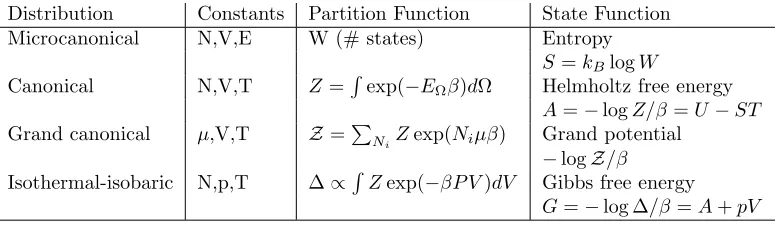
we are at low (atmospheric) pressure,pV is negligible compared toU and so H _≈U andG_≈A. Distribution Constants Partition Function State Function

Microcanonical N,V,E W (# states) Entropy

S=kBlogW

Canonical N,V,T Z=Rexp(₋EΩβ)dΩ Helmholtz free energy

A=₋logZ/β=U₋ST

Grand canonical µ,V,T Z=P_N_iZexp(Niµβ) Grand potential −log_Z/β

Isothermal-isobaric N,p,T ∆_∝R Zexp(₋βP V)dV Gibbs free energy

[image:15.595.105.496.528.641.2]

G=₋log ∆/β=A+pV

Table 1.1: A list of the common thermodynamic distributions, their constants, partition functions and macroscopic state functions. µis the chemical potential defined as∂A/∂N when volume and temperature are kept fixed.

(16)

1.1.3 Phase Transitions

From an intuitive perspective, phase transitions are abrupt changes of macroscopic properties of a system with changing external conditions. For example, the decrease in temperature of a liquid can lead the system to freeze into a solid, and lowering the temperature of a paramagnetic material below its Curie point causes an abrupt transformation from paramagnetism to ferromagnetism, i.e. having a magnetic moment. Phase transitions also occur in more abstract branches of science; for example, in random graph theory, as the probability of edges increases above a critical threshold, the probability of there being a single connected component abruptly approaches 1. Mathematical theories, for example Mean– field theory and Ginzburg-Landau theory, have been developed in order to explain the behaviour of systems at phase transitions and we refer the reader to standard texts for full descriptions (2, 4).

From a (constant NVT) statistical mechanics perspective, a phase transition occurs when the Helmholtz free energy is non-analytic. If the first derivative ofAis discontinuous, then the phase transition is first order, whereas if the first derivative is continuous but its second derivative is discontinuous, then the transition is described as second order. Examples of first order transitions include the melting of ice and boiling of water. Examples of second order phase transitions include the ferromagnetic transition from paramagnetism to ferromagnetism. Figure 1.1 shows the behaviour of the internal energy and heat capacity of systems with first and second order phase transitions. Analogous behaviour can be found for systems in the isobaric-isothermal distribution withGreplacingA.

T

c

T

c

U

C

_v

T

c

T

c

U

[image:16.595.134.468.359.676.2]

C

_v

Figure 1.1: Left: Behaviour of the internal energy (top) and heat capacity (bottom) of a system with a first order phase transition at temperatureTc. Right: Behaviour of the internal energy (top) and heat

capacity (bottom) of a system with a second order phase transition at temperatureTc.

(17)

The phase transitions described above involve bulk systems with enormous numbers of degrees of freedom, yet these systems cannot be modelled computationally in atomic detail. Only the behaviour of smaller (or periodic) systems with fewer degrees of freedom can be studied computationally. These systems, or indeed any finite system, cannot exhibit a true first order phase transition, with a genuine discontinuity in internal energy. They can, however, exhibit a quasi-first order transition, where theCv

curve is sharply peaked but remains finite and theUversusTgraph is sigmoidal rather than discontinuous (Figure 1.2 (left)). Typically as N, V _{→ ∞} with N/V remaining constant, the transition becomes ‘sharper’, i.e. theCvpeak is higher and occurs over a shorter temperature range, and rapidly approaches

a true first order transition in the thermodynamic limit.

Finally, we consider how the probability distribution of the potential energy behaves at a first order phase transition (5). Firstly, away from the phase transition, it can be shown that the distribution is Gaussian, with mean U(T) as shown by Figure 1.2 (a,e). Near the critical temperature, Tc, the

distribution is no longer unimodal and non-negligible probability mass is found around two separate energy valuesUX andUY, the average energy of the system at this temperature, given that the system is

restricted to phase X or respectively Y. This is shown by Figure 1.2 (b,d). AtTcthe probability of being

found in phase X is exactly a half as shown in Figure 1.2 (c). AtTc the free energy of the small number

of low energy states of phase X exactly balances the free energy of the large number of high energy states of phase Y. As we show below, this behaviour causes serious difficulties when computationally sampling from such a system.

Figure 1.2: Left: The internal energy (U) as a function of temperature for a system exhibiting a quasi– first order transition at temperature Tc. Right: The potential energy probability distribution for this

system at five different temperatures A)T Tc B) T < Tc C)T =Tc D)T > Tc E)T Tc

1.2 Sampling of Atomistic Systems

Given a molecular model and potential energy functionEΩ, we are often interested in calculating kinetic and thermodynamic properties of the system, in order to compare to an experiment, to compare to other, often similar, systems or to provide new insight into how the system behaves when changing its external conditions. Kinetic, or dynamic, properties of the system, such as diffusion and equilibration rates, are

(18)

time-dependent properties, whereas thermodynamic averages, such as free energies, are time-independent properties of the system when it is in equilibrium. In order to calculate these properties, it is necessary to evolve the state of the system and draw samples for analysis.

In this section we introduce the important sampling techniques of molecular dynamics and Monte Carlo sampling. We then describe the sampling problem associated with sampling from Boltzmann distributions and discuss methods which attempt to solve this problem. We end the section with a description of nested sampling, a new sampling technique developed for Bayesian inference, which has shown potential for improving the sampling of atomistic systems.

However, we first briefly mention molecular models and their energy functions. A model of a molecule consists of a series of atoms and information as to how they are covalently bonded, together with a set of parameters such as atomic charges, bond lengths and valence angles. A model of a system consists of a set of molecule models together with details of boundary conditions, system volume, size and shape.

The potential energy function of physical models comprises of three separate terms

EΩ=EbondedΩ +Enon-bondedΩ +EexternalΩ .

Ebonded

Ω captures the energetic interactions between covalently bonded atoms. These interactions include bond stretching, usually modelled with a harmonic function, valence angle bending and bond rotations.

Enon-bonded

Ω captures interactions between non-covalently bonded atoms, for example, electrostatic inter-actions, using a Coloumb potential, and van der Waals interinter-actions, often modelled by a Lennard Jones (LJ) potential.2 _Eexternal

Ω consists of terms external to the set of atoms, such as the energy from an external magnetic field. We discuss specific models for proteins in_§1.3.4 and the reader is referred to (6) for more details of general molecular models.

1.2.1 Molecular Dynamics Sampling

First developed computationally in the late 1950s by Alder and Wainwright (7), molecular dynamics (MD) evolves the state of the system by integrating Newton’s equations of motion. Given the potential energy functionEΩ, initial atomic co-ordinates Ω(0) ={xi(0)} and velocities{vi(0)}, we have

mi

d2_xi

dt2 =Fi,

where the forces Fi are given by−∇xiEΩ(x). Solving this system of differential equations leads to a

trajectory Ω(t).

It can be shown that the total energy (EΩ+kinetic energy) of the trajectory remains constant, and therefore, assuming the ergodic hypothesis described below is satisfied, the samples generated are dis-tributed according to the microcanonical distribution.3

When integrating the equations numerically, care must be taken to use an integration scheme which does not introduce large discretization errors. Schemes such as the Verlocity Verlet, described in (8), are widely used.

In the thermodynamic limit of a large number of particles, the canonical and microcanonical ensembles coincide. However, for small systems, in order to sample their canonical distributions, a thermostat must

2_{If atomic distance is}_{r, then the LJ potential is given by 4((σ/r)}12₋_(σ/r)6_{) where} _and_σ _{are parameters. The} LJ potential models both short-range repulsion and the long-range attraction due to the fluctuating charge densities of induced dipoles.

3_{Technical details have been omitted. For example, in non-periodic systems the angular momentum,} _{J, is also a} constant of motion and samples come from a ‘NVEJ’ distribution.

(19)

be used to ensure constant temperature. The Andersen thermostat (9) is a simple procedure, coupling the system to an external heat bath to maintain the desired temperature. After each timestep, each atom undergoes a collision with the heat bath with probabilityν. A collision involves resampling the momentum of an atom, with its new momentum sampled from the Maxwell-Boltzmann distribution4 _at the desired temperature. It can be shown that the samples generated using this procedure come from the canonical distribution.

Other schemes, such as Langevin dynamics or the Nos´e–Hoover thermostat, have also been developed. For further details on these and sampling atomistic systems in general, we refer the reader to the excellent discussion in (10). Barostats, which control the pressure of the system by changing its volume, have also been developed, enabling isothermal-isobaric trajectories to be computed.

When using MD trajectories to estimate kinetic properties of the system, for example diffusion rates, it is important to choose a thermostat and barostat which preserve the kinetics of the system. The resampling of momenta in the Andersen thermostat described above means it cannot be used to estimate time-dependent system properties.

As well as the calculation of kinetic properties, samples from MD trajectories can be used to estimate thermodynamic averages. For example, given an NVT trajectory Ω(t), . . . ,Ω(M t), the thermodynamic energy can be estimated as

hEΩiβ≈

1

M

X

i=1

EΩ(it)

and this will, in the limit of largeM, converge to the ensemble average, assuming the ergodic hypothesis. The ergodic hypothesis, originally formulated by Boltzmann at the end of the 19th century, proposes that the long-time average of a property over a trajectory does indeed converge to its ensemble average. Whilst usually assumed true, there are cases when, in practice, it does not hold, such as when the system has long-lived metastable states.

1.2.2 Monte Carlo Sampling

An alternative to MD simulation is that of Markov Chain Monte Carlo (MC) sampling. The MC method was devised in the 1940s and ’50s for use on some of the very first computers. We refer the reader to (11) for an interesting historical perspective on the invention of MC methods.

The basic idea of this method is to devise a Markov chain,5 _{such that its equilibrium distribution is} the distribution from which we wish to sample. Again, assuming ergodicity, ensemble averages can then be estimated from the MC samples.

We describe the Metropolis-Hastings algorithm (12), a generalization of the original Metropolis pro-cedure (13). In order to use this method, a set of moves which evolve the state of the system must be devised. We define _P(Ω _→ Ω0_{) as the probability that, given conformation Ω, a move is chosen} which would transform it into conformation Ω0. Assuming the system is in conformation Ω and we have proposed to evolve the chain to conformation Ω0_{, we accept this move with the Metropolis-Hastings} acceptance probability

min

1,P(Ω

0₎_P_(Ω0_→_Ω)

P(Ω)P(Ω_→Ω0₎

,

where P(Ω) is the distribution of interest. In the case of the canonical distribution, P(Ω0)/P(Ω) =

4_{The marginal distribution of momenta when the system follows the canonical distribution.} 5_{A Markov Chain is a sequence of random variables}_{X1, X2, . . .}_{such that}_P_(X

k|Xk−1, Xk−2. . . , X1) =P(Xk|Xk−1). In atomistic systemsXiis a conformation Ωi.

(20)

exp(−β(EΩ0 −EΩ)). If we reject the move, the MC chain remains in state Ω and another move is proposed. The equilibrium distribution of this chain isP(Ω).

The choice of the move set is an important factor in MC procedures. Since onlyEΩ0 −EΩis required in order to accept or reject moves, local moves, that is those which keep most of the system fixed, are usually more efficient; only the part of the potential energy function which involves the atoms that have moved needs to be calculated for each iteration. Also, at low temperatures, large changes to the system will likely be rejected. In atomistic systems, moves typically include molecular translations and rotations and intra-molecular bending and rotation of covalent bonds.

Alongside canonical sampling, the MC procedure has been used to sample other thermodynamic distributions, as described in (10). These even include the grand canonical ensemble, where proposal moves include the addition or removal of atoms from the system.

Unlike MD sampling, samples generated from an MC sampler cannot be used to estimate kinetic properties of the system but, if appropriate moves exist, MC sampling can be a very efficient way of exploring conformation space.

1.2.3 Advanced Sampling Techniques

Unfortunately, in many cases standard MC or MD sampling is not effective. For example, in a multimodal system with low probability of swapping between modes at temperatureβ, the system will become stuck in a single mode and require an enormous runtime in order to produce accurate ensemble averages.

If we are using MD or MC to sample a system with a phase transition near the critical temperature, for example Figure 1.2 (right C), it will be nearly impossible to equilibrate the samples between the (relatively) small number of low energy samples with energy around UX and the large number of high

energy samples with energy nearUY. This problem can occur in both multi and unimodal systems. We

return to this example in more detail below.

Furthermore, if the partition function is required, it is possible to use the samples, Ω1, . . .ΩM to

produce an estimate

Z−1=_hexp(EΩβ)iβ ≈ m

X

i=1

exp(EΩiβ).

However, this estimate, the ‘harmonic mean approximation’, has infinite variance at low temperatures (14) and hence should not be used.

In order to avoid these problems, more sophisticated sampling algorithms involving MC, MD or a combination of both techniques have been designed. In this section we discuss some of these algorithms before introducing a novel algorithm, nested sampling, which has the potential to significantly improve the sampling of atomistic systems.

General Sampling Algorithms

Although technically an optimization algorithm, we first describe simulated annealing (SA), as the ideas it introduces are applicable to the sampling algorithms described below. SA was developed by Kirkpatrick and colleagues in the early 1980s (15). The algorithm starts by exploring the conformation space using a high temperature canonical MC chain. Gradually throughout the simulation, the temper-ature is lowered, following a chosen schedule, until we are sampling from the canonical distribution of the temperature of interest.

At high temperatures (lowβ), the factor exp(−EΩβ) is less important: in the limit of high tempera-ture this term is constant with respect to EΩ, and exploring is easy, as it is uniform in conformational

(21)

space. At the start of SA, the chain can explore the conformation space more easily and thus larger MC steps can be taken. As the temperature is decreased this exponential factor becomes more important and smaller MC steps must be taken. The system is slowly cooled, hopefully resulting in finding the correct (free) energy minimum of the system. The slow cooling gives the a system chance to properly equilibrate.

Once the temperature has been reduced, the conformation will eventually become stuck in a local minimum. An adaptation of SA, the simulated tempering algorithm (16), allows increases of the tem-perature of the system, so that the conformation is no longer trapped. Thus, when the temtem-perature is lowered again, the system can explore another minimum.

One of the most widely used sampling algorithms is that of parallel tempering (PT). It was first developed by Swenson in 1986 (17) and, like SA, the temperature of the system becomes a parameter of the algorithm. In the PT procedure, a set of separate MC chains (replicas) are run at different temperatures in parallel. Periodically one proposes that the temperatures of two chains are swapped. This proposal is accepted using an acceptance criterion similar to the Metropolis-Hastings criterion described above.

A key advantage of this approach is that multimodal systems can be sampled much more efficiently. Low temperature replicas, which would have been be trapped in local modes, can ‘escape’ by swapping with a conformation from a chain with higher temperature. The high temperature replicas can themselves more easily escape modes, as explained above.

The algorithm outputs samples from the canonical distribution at a variety of temperatures which can be used to produce thermodynamic averages over a range of temperatures. Thermodynamic estimates for other temperatures can also be estimated from these samples using a procedure such as Boltzmann reweighting (18).

However, care must be taken to ensure enough replicas are used (order√Nfor system sizeN), so that the probability of accepting proposed temperature swaps is not too small. Also, the set of temperatures used must be chosen with care. For example, at a phase transition, more replicas are needed near the critical temperature to ensure proper equilibration, even though the existence and location of the transition is not knowna priori.

Replica exchange molecular dynamics (REMD) (19) is the same algorithm as PT, except that instead of each replica running an MC chain, it follows an MD trajectory. Care must be taken to rescale the velocities after replicas have been exchanged. REMD affords the benefits of PT for systems for which MC moves are not as efficient as MD.

REMD and PT are widely used algorithms, and various adaptations and improvements have been developed, for example, adapting the temperature of replicas throughout the simulation in order to maximize efficiency (20). For a general overview of PT and REMD, consult (21).

Alternative ways of combining MC and MD sampling have also been researched. As an example, we describe the Hybrid Monte Carlo (HMC) algorithm of Duane et al. (22). The HMC algorithm is a special MC chain, whereby proposal conformations are generated by giving the atoms of the current conformation momenta and then running a short MD trajectory.

Perhaps counterintuitively, rather than sampling the canonical distribution directly, it may be more efficient to sample from a non-canonical distribution and then weight samples to estimate canonical thermodynamic averages. Algorithms which follow this approach are named biased or extended ensemble sampling methods. As an example we describe the multicanonical sampling algorithm (23). For this method, instead of attempting to sample conformations ∝ exp(−EΩβ), we sample ∝ 1/g(EΩ) where

g(E) =R_Ωδ(EΩ−E)dΩ is the density of states (δ is the Dirac delta function).

(22)

This choice of distribution implies that the histogram of potential energies of the samples will be flat, so that the system is sampling ‘uniformly in energy’. This has the advantage of removing the exponential barrier between different modes which is found with canonical sampling algorithms. However, before being used, the algorithm requires a learning stage in order to estimate g(EΩ) and, as the system size increases, the number of parameters which need to be estimated in order to resolve g(EΩ) accurately can cause problems.

The challenge of estimatingg(EΩ) can be overcome by a powerful non-Markovian (history-dependent) algorithm, the Wang-Landau sampling algorithm (24), which interactively changes the Markov accep-tance criteria to ensure that the system converges to the 1/g(EΩ) distribution.

As the exploration of phase space is such an important problem both in atomistic systems and statistics in general, many other sampling algorithms and combinations of existing algorithms have been developed. Examples include equi-energy sampling (25) and the 1/k ensemble algorithm (26), a variant of the multicanonical sampling algorithm, notable in this work because it aims to sample conformations uniformly in log phase-space volume rather than energy. We now, however, turn our attention to sampling algorithms specifically developed for calculating the partition function or free energies of atomistic systems.

Partition Function and Free Energy Estimation Algorithms

Within the statistical literature, algorithms have been developed for calculating the marginal like-lihood (partition function) of models. Examples include annealed importance sampling (27), Laplace’s method (28) and bridge and path sampling (29). Interesting discussions from a statistical viewpoint can be found in (29, 30). Here, however, we focus on methods developed for atomistic systems. Rather than specific values of free energies themselves, statistical physicists are typically more interested in free energy differences, either between two separate systems or between macrostates within the same system. Unlike thermodynamic variables such as the heat capacity, which can be calculated directly as en-semble averages, free energies are related to volumes in conformation space (consider the definition given in_§1.1.2). This makes their calculation more challenging.

One of the most common methods for calculating free energy differences is that of thermodynamic integration (TI) (31). As a simple example of TI, consider the case of two systems X andY, identical apart from the fact that X has potential energy functionEX

Ω and Y has potential energy functionEYΩ. Introducing a parameterλand defining a new potential energy function

EΩλ = (1−λ)EΩX+λEΩY

it can be shown that the free energy difference between systemsX andY is given by Z 1

0

dλ

_∂U₍_λ₎

∂λ

λ

.

The integrand is an ensemble average which can be estimated through MC or MD sampling for different values ofλ, and numerical integration can then be used to estimate the free energy difference.

Often, it is of interest to calculate how the free energy of a system changes when a reaction co-ordinate, a chosen function of the atomic co-ordinates such as an atomic distance or angle, is used. The free energy surface along such a co-ordinate is known as the potential of mean force (PMF) (32). PMFs can be challenging to compute if the surface contains high free energy barriers.

Umbrella sampling (33) is traditionally used to calculate PMFs. In this method, an extra biasing

(23)

potential is used to force the system to sample a chosen value of the reaction co-ordinate. The procedure is then repeated for different values of the reaction co-ordinate and reweighting these samples generates a more accurate PMF compared to naive MD or MC sampling. In order to further improve the efficiency of the procedure, more sophisticated reweighting techniques, such as the weighted histogram analysis method (WHAM), have been applied to the calculation of PMFs (34).

There have also been many other approaches to the calculation of free energies, including thermo-dynamic perturbation (35), approximate rapid methods such as λ-dynamics (36) and more specialist algorithms specifically for the calculation of free energies of solids (37).

Nested Sampling

Nested sampling is a novel sampling algorithm invented by Skilling in 2004 in order to estimate the marginal likelihood (i.e. the partition function) in Bayesian inference problems (38, 39). The algorithm is designed for models for which the bulk of the posterior probability mass is contained in an exponentially small area of the prior space. It is particularly efficient at sampling systems which undergo first order phase transitions. The algorithm has been used in a wide variety of fields, including astrophysics (40), system biology (41) and bioinformatics (42).

As shown in _§1.1.1, Bayesian inference algorithms can be applied to atomistic systems, and nested sampling has been shown to be an order of magnitude more efficient at calculating heat capacity curves of small Lennard Jones clusters compared to parallel tempering (43). The nested sampling algorithm is

athermal, and when run, produces samples from throughout the whole potential energy surface of the system. These samples can be used to estimate thermodynamic variables at any temperature. P´artay

et al. have used these samples to generate energy landscape charts, which give a high-level visualization of the potential energy surface. They have also used these charts to define macrostates of the system without having to pick specific reaction co-ordinates (43).

A simple description of the algorithm follows below and more details and in-depth discussions can be found in Chapters 2, 5 and 6 of this work. The algorithm begins by choosingK samples uniformly distributed according to the prior distribution, which in the case of atomic systems is uniform over conformation space. These samples are the current ‘active set’ and the energy of each sample is calculated. The conformation with the highest energy is removed from the set and its energy,E1is saved. A new conformation, uniformly distributed over the set of conformations with energy less thanE1 is generated and the procedure continues, generating a series of energy levelsE1, E2, E3. . ..

The algorithm does not prescribe how exactly to generate a sample uniformly distributed with energy below Ei. One method involves making a copy of one of the conformations in the active set and then

running a MC chain to move the copy away from its starting point. In order to sample uniformly, the standard Metropolis-Hastings acceptance criterion is replaced by a simple criterion: accept the moveiff

the energy remains below the current energy cutoff, assuming the moves are such that the probability of proposing Ω_→Ω0 _{and Ω}0 _→_{Ω are the same.}

As explained below, one of the key advantages of nested sampling is that the phase space is shrunk by a constant factor, α, at every iteration. By using the expected value of the shrinkage ratio, we can estimate α_≈exp(₋1/K). Estimates forα which take into account the statistical uncertainties of the procedure can also be used.

By definingXi=αi, energy levelEiand the conformation removed at this energy level (Ωi) represent

a fractionωi =Xi−1−Xi of the prior (conformational) space and, at inverse temperatureβ, represent

a fraction χi(β) =ωiexp(−Eiβ)/Z(β) of the posterior (Boltzmann distributed) space. The partition

(24)

function is estimated by numerical integration as

Z(β)≈X i

ωiexp(−Eiβ).

The expected value of any thermodynamic observable,Q(Ω), at any temperature can also be estimated as

E(Q_|β)_≈X

i

χi(β)Q(Ωi)

The algorithm terminates when a specific criterion is reached, for example, the estimate for Z(β) has converged for the temperature of interest. Other criteria may be more appropriate for some systems (39). Algorithm 1 summarizes the nested sampling algorithm.

Algorithm 1The Nested Sampling Algorithm

1) SampleKconformations uniformly (w.r.t. conformation space),_{Ω1,Ω2, . . .ΩK}and calculate their

energies_{EΩ1, EΩ2, . . . EΩK}.

2) Remove the conformation with highest energy from the active set; save it as (E1, X1,Ω1).

3) Generate a new conformation Ω, sampled uniformly from the conformations with energy belowE1, and add it to the active set.

4) Repeat Steps 2 and 3, generating (E2, X2,Ω2),(E3, X3,Ω3), . . ..

Sampling techniques such as parallel tempering and simulated annealing struggle to sample systems which undergo first order transitions, such as the system shown in Figure 1.2. Starting at diagram E, SA has to find the volume of phase space with energyUx which has non-negligible probability mass. This

volume is exponentially small in comparison to the phase space of conformations with energy UY and

in some cases it can be effectively impossible to find it. Furthermore, going from diagram D to A, the proportion of samples from each Gaussian needs to be kept in equilibrium. Added to this, the fact that the temperature of the phase transition is not knowna priori means the temperature schedule may miss the transitions entirely. Similar concerns exist for PT. There may be no replicas with temperature near

Tc, and even if there are, for example if an adaptive temperature schedule is used, it can still be very

hard to equilibrate.

Phase transitions, however, are not a problem for nested sampling, which takes steps equidistant in log phase space volume, taking smaller steps (in energy) when the space shrinks more quickly. It just marches down fromUY toUX, unaware that there was a problem for thermal methods.

In this section we have considered a variety of sampling algorithms without discussing their application to research problems. In_§1.3.6 and_§1.3.7 we discuss the application of these algorithms to the study of proteins and the results they have produced. For more details of general atomistic sampling, however, we refer the reader to (10) and references therein.

1.3 Proteins: Modelling and Applications

1.3.1 Overview

Proteins are essential to life. Some are enzymes, catalysing cellular chemical reactions. Others are antibodies, recognising pathogens. Yet more control transport into and out of cells or sense and act on signals generated by the organism or environment. Regulatory proteins regulate and control cellular processes such as gene transcription; structural proteins, such as keratin and actin, form tissue such

(25)

as skin and muscles; and motor proteins convert chemical energy to mechanical energy, for example in muscle contraction. The incorrect behaviour of proteins is implicated in a large range of disease such as Alzheimer’s or Type II diabetes. The intricate three-dimensional structures of proteins are finely tuned, through evolution, to perform their highly specialised functions. The diverse structures proteins adopt explain the large variety of functions they are able to perform.

Protein science, the study of these molecules, is a very wide field, encompassing theory and techniques from chemistry, molecular and cellular biology, evolutionary biology, bioinformatics, computer science and biophysics (44). Over the last 70 years proteins have been studied both experimentally, using techniques including X-ray crystallography (45, 46), NMR spectroscopy (47), circular dichroism (48) and fluorescence resonance energy transfer (FRET) (49); and computationally, from simple lattice models (50) through to full all-atom models with more realistic force fields (51).

In this work we mainly focus on globular (water-soluble) proteins. However, there is another impor-tant class of proteins: membrane proteins. Membrane proteins are found in water-deficient environments and hence are subject to different conditions to globular proteins and so behave differently. For example, exposed charges, whilst often favourable in water, are severely energetically disadvantageous when in contact with a hydrophobic (‘water-hating’) membrane.

The following sections describe the structure of proteins, the theory of protein thermodynamics, the different types of protein models used to study proteins computationally, how the parameters of these models are inferred and how conformations are sampled using them. Finally, there is a summary of applications of protein models. However, discussion of an important application, that of protein structure prediction, is deferred until later.

1.3.2 Protein Sequence and Structure

The building blocks of proteins are amino acids and there are 20 standard,proteinogenic amino acids. With the exception of one, proline, all have a standard molecular structure (Figure 1.3 (left)) shown with the standard atom names), differing only in their side chain. For example, glycine (code G) has a single hydrogen side chain, whereas serine (S) has a side chain CH2-OH. The side chain of proline (P) covalently bonds to both theCα and N atoms; see Figure 1.4. Different side chains endow the amino

acids with different properties. For example, some amino acids are hydrophobic (‘water-hating’) and others are hydrophilic (‘water-loving’).

A protein is a linear sequence of amino acids joined by peptide bonds (Figure 1.3 (right)) forming a protein chain. Short protein chains are called peptides. Proteins are defined by a specific sequence of amino acids (also called residues). An organism’s protein sequences are encoded within its DNA. The repeating -(N-Cα-C0)- pattern denotes the protein backbone and the two ends of the protein are called

theN andC termini.

Over 50 years ago, the chemist Linderstrøm-Lang described a hierarchy of protein structure (53), the primary, secondary and tertiary structure of a protein; these terms are defined below. A further level, the quaternary structure, was later added to describe how separate protein chains assemble into larger structures.

The primary structure, or sequence, of a protein is precisely an ordered list of its constituent amino acids. Due to the polar nature of the N-H and C-O covalent bonds (H is slightly positively charged, O negatively so), an electrostatic ‘hydrogen bond’ can form between water and a residue or between two different residues. Certain intra-protein hydrogen bond patterns are energetically favourable and hence common motifs, α-helices and β-strands, are found in most proteins. The specific pattern of helices,

(26)

Figure 1.3: Left: The molecular structure of an amino acid. The atoms are labelled with their standard names and R represents the amino acid side chain. Right Top: A protein is a linear sequence of amino acids and the ends of the protein are called theN andCtermini. Right Bottom: The first two residues of a protein joined by a peptide bond (in green) between C0 _{of residue 1 and}_N _{of residue 2. All atomic} models have been created using VMD (52).

Figure 1.4: Unlike the sidechains of the other amino acids, which are only bonded to the Cα atom,

the side chain of proline, as shown, covalently bonds to both Cα and N atoms. Therefore, proline is

technically an imino rather than amino acid. In amino acids the side chain atoms are labelled with the

β-atom bonded to the backbone Cα atom, theγ-atom bonded toβ-atom etc. The Cβ, Cγ and Cδ atoms

of proline are labelled.

strands and coil (other) residues is the secondary structure of a protein.

In an α-helix, the hydrogen atom from residue i bonds with the oxygen atom of residue i−4; continuing this pattern leads to a helix with 3.6 residues per turn, as shown by Figure 1.5 (left). Other helices, whilst significantly rarer, are also found in proteins, specifically, 310-helices, where the bonding pattern is i→i−3; andπ-helices, which have bonding i→i−5. Aβ-strand is typically a sequence of 5-10 residues hydrogen bonded with a set of consecutive residues elsewhere in the protein. β-strands can hydrogen bond in parallel or anti-parallel directions and when bonded formβ-sheets; see Figure 1.5 (right).

The reasonα-helices andβsheets are energetically favourable can be understood in terms of backbone dihedral anglesφandψand the Ramachandran plot. The dihedral angle of a chain of atomsa1, a2, a3, a4 is the angle between the planes containing a1, a2, a3 and a2, a3, a4. In a protein, φi is defined as the

dihedral angle between C0-N-Cα-C0, ψi between N-Cα-C0-N and ωi between Cα-C0-N-Cα, where i runs

over the residues of the protein. See Figure 1.6 (left). Due to the nature of peptide bonds, the four atoms{Cα,C0,N,Cα}are always close to planar and henceωis always close to 180◦(transconformation)

or 0◦ ₍_cis _{conformation).}

(27)

[image:27.595.150.446.72.278.2]

Figure 1.5: Left: A cartoon picture showing anα-helix and the corresponding full atom representation. Right: A cartoon picture showing a pair of anti-parallel β-strands with the corresponding full atom representation. Only main chain and Cβ atoms are shown. The backbone atoms are highlighted and the

hydrogen bonds are coloured orange.

With the exception of proline residues, thecisconformation is extremely rare due to the energetically unfavourable steric repulsion of consecutive Cαatoms when compared to thetrans case in which the Cα

atom is close to the much smaller amide hydrogen. The special nature of the proline sidechain makes the

cis conformation much less unfavourable, as in thetrans case the small hydrogen atom is now replaced by the massive Cδ atom (see Figure 1.4). Around 10% of peptide bonds preceding proline residues are

found in thecis conformation.

Unlikeω,φandψare allowed to vary and provide most of the conformational freedom of the protein main chain. A Ramachandran plot is a graph showing the dihedral angles of a protein (Figure 1.6 (right)). Only certain regions of the graph can be occupied, as dihedral angles from other regions would lead to steric clashes between backbone or Cβ(the carbon atom in the side chain bonded to Cα) atoms.

Both theα-helix andβ-strand have standard dihedral angles which are in the sterically allowed regions of the graph. Both proline, with its special sidechain, and glycine, which lacks Cβ and hence has more

freedom, have different allowed regions to other amino acids. Certain local motifs of secondary structure elements, such as aβ-hairpin (two anti-parallelβ-strands connected by a short turn) or aβ-α-βunit (two interacting parallelβ-strands separated in sequence by a single helix), are frequently found in proteins, and these motifs are often called the ‘supersecondary’ structure.

The tertiary structure of a protein is how the secondary structure elements combine to form the full three dimensional structure. The tertiary structure is determined by many factors. These include the hydrophobic effect; non-polar side chains being buried in the core of the protein away from the solvent (54, 55); electrostatic charges, both involving hydrogen bonds and salt bridges between charged amino acids (56); dense side chain van der Waals packing (57); the existence of metal ions (58) and disulphide bridges, where the sulphur atoms of two cysteine (C) amino acids form a covalent bond (59).

Typically large single chain proteins are composed of domains, single subunits capable of folding independently of the rest of the chain, connected by somewhat disordered loops. Certain domain folds are particularly common, such as the three helix bundle. For the last 20 years, domain structures have

(28)

Figure 1.6: Left: The dihedral angles φ,ψ and ω. Right: A Ramachandran plot showing the dihedral angles of protein G (Figure 1.11 (left)). The shaded blue regions are the most stable; whereψis positive this indicates a β-strand and when it is negative, an α-helix. The shaded green regions are allowed but more strained. The yellow areas are less favourable due to steric clashes and are significantly less common. Glycine, with its smaller sidechain, has more freedom than other amino acids, and the glycine residues of protein G have been highlighted in red.

been classified and databases of them maintained (60, 61).

In this work we focus on the large number of proteins which have well-defined tertiary structure essential for their function. Since the pioneering work of Anfinsen and colleagues (62), it has been understood that proteins (at least small, globular proteins) fold into their tertiary (native) structure reversibly, leading to the conclusion that the structure of a protein is fully encoded in its primary sequence and that the native state is thermodynamically stable. However, recently, there has been a lot of interest in intrinsically disordered proteins, that is proteins which do not adopt a well defined structure, until, say, they bind to a ligand; they are now believed to be significantly more numerous and important than originally thought (63, 64).

1.3.3 Protein Thermodynamics

In 1969 the molecular biologist Cyrus Levinthal asked the question: how can a protein fold into its native state in the millisecond to second timescales that are observed? For simplicity, assume each residue can take two possible states, α-helical orβ-sheet. Then a 100 residue protein would have ≈1030 possible conformations, and assuming an interconversion rate of _∼ 10−13_s_{, it would take of the order of 10}10 years for the peptide to explore its conformational space. This argument, named the Levinthal paradox, implies that protein folding is not a simple diffusive process, and this has lead to the idea of a protein folding funnel (65–68).

Protein Folding Funnel

The free energy landscape of a system behaving according to Levinthal’s diffusive process is shown by Figure 1.7 (left). With the exception of the native state, the landscape is flat and hence a random search is required in order to ‘stumble upon’ the native state. In contrast, Figure 1.7 (right) shows a

(29)

[image:29.595.150.448.131.432.2]

protein folding funnel. The protein starts from one of a large number of conformations with high energy and hence has high entropy. The chain decreases in energy towards the native state, a state with low entropy.

Figure 1.7: Left: The free energy landscape of a system behaving according to Levinthal’s diffusive process. With the exception of the native state, the landscape is flat and hence a random search is required in order to ‘stumble upon’ the native state (N). Right: A protein folding funnel. The protein starts from one of a large number of conformations with high energy and entropy. The chain decreases in energy towards the native state (N), a state with low energy and entropy.

A realistic folding funnel of a naturally occurring protein has rugged sides corresponding to metastable states or kinetic traps which slow the steady march of the protein toward its native state. The free energy difference between the native state and other free energy minima is of the order of 10 kcal/mol (69), which equates to only a couple of hydrogen bonds. This implies that naturally occurring proteins are only marginally stable, which has been shown to be evolutionarily advantageous (69). In contrast, randomly chosen heteropolymers typically have very rugged energy landscapes with no clear native state: the free energy gap between the global minima and other minima is small and the dynamics are glassy (70).

One theory of protein folding is the hierarchical folding theory of Baldwin and Rose (71, 72). Accord-ing to this theory, a protein folds by first formAccord-ing local secondary structural elements such asα-helices andβ-strands, and then these structures interact with each other to form the native structure.

Initially the unfolded protein collapses from an extended chain into a ‘molten globule’ state. At this time the protein is relatively compact, has a substantial amount of correct secondary structure and yet has more flexibility and looser hydrophobic packing compared to the native state. In order to form the native state, the secondary structure elements come together, forming a tighter hydrophobic core with the amino acid side chains interlocking tightly.

(30)

In order for the native state to form, the protein has to overcome free energy barriers (66) in a similar way to chemical reactions requiring an activation energy in order for the reaction to proceed. The free energy barriers correspond to regions of increasing free energy on the free energy landscape, which must be traversed in order to reach the native state. The conformations at these local maxima are called transition states.

From an experimental point of view, it is not possible to visualise the high dimensional free energy landscape. However, protein folding pathways can be investigated through a procedure known as Φ-analysis (73). Φ-Φ-analysis allows investigation of the transition state, which is by definition unstable and short lived and therefore not amenable to standard structural methods.

Figure 1.8 (left) shows a reaction diagram for a non mutated (wild-type) protein. Although the free energy of the native state is lower than that of the unfolded state, in order for the protein to fold, activation energy is required in order to reach the transition state. If a residue is making the same interactions in both the native state and the transition state then, when it is mutated, both the transition and folded states are destabilized by similar amounts, as shown in the reaction diagram Figure 1.8 (middle). However, if the residue is not making the same interactions, then only the folded state is destabilized and the reaction diagram Figure 1.8 (right) is seen. The ratio of the destabilization of the transition state to the destabilization of the native state, Φ = ∆∆G‡_/_∆∆_G_{, can be measured for} different residues by estimating rate constants, and these results can be used to build up a picture of the transition state.

Transition

ΔΔG ΔΔG

ΔΔG

ΔG

Unfolded

Transition

Folded

Unfolded

Folded

Unfolded

Folded

Figure 1.8: Left: A reaction diagram for a non-mutated (wild-type) protein, where a free energy barrier of height ∆G‡ _{must be overcome in order for the protein to fold. Middle: The reaction diagram of} the protein when a residue which has the same interactions in both the native state and the transition state has been mutated (red). The transition and folded states are destabilized by similar amounts and Φ = ∆∆G‡/∆∆Gis close to 1. Right: The reaction diagram of the protein when a residue which does not have the same interactions in both the native state and the transition state has been mutated (red). The folded state is destabilized significantly more than the transition state and Φ is close to 0.

The situation described by Figure 1.8 (left) is the most simple case. Many proteins have more complicated reaction diagrams, including meta-stable intermediate states, corresponding to local minima of the free energy landscape, and even multiple folding pathways, whereby a different folding rate is attained depending on which folding pathway is taken.

Finally, from a statistical thermodynamics viewpoint, there are theoretical arguments suggesting that denaturation of globular proteins is a (quasi) first order phase transition (74); experimental evidence such as circular dichroism spectra (75) and experimental heat capacity curves (76) also supports the conclusion that the transition is all-or-none. This first order transition has implications for the sampling of protein conformations in silico. The nature of this transition explains the free energy barriers and activation energy required for a protein to fold. For further discussions concerning protein thermodynamics we refer the reader to (77).

(31)

It is very useful to form general theories about protein folding and thermodynamics. However, it is important to note that the complex balance of competing forces can produce very different behaviours in different proteins and that these sequence-specific details are of crucial importance. For example, ubiquitin is a 76 residue protein with a folding rate of_∼3ms, whereas the 73 residue proteinα3D folds around three orders of magnitude faster at _∼ 3µs (78). Equally noteworthy, Karanicolas and Brooks have shown that two proteins with the same native fold follow very different folding pathways, with protein G initially folding its C terminal hairpin, in contrast to protein L which first folds its N terminal hairpin (79).

1.3.4 Protein Models

In the 1950s, Linus Pauling and Robert Corey used simple protein models to predict the existence of

α-helices andβ-sheets before they were discovered experimentally (80). Since that time protein models have continued to improve our understanding of protein structure, stability and thermodynamics. Early models, such as the HP lattice model of Lau and Dill (50), gave an insight into the general principles of protein folding, rather than protein-specific details.

In the HP model, each residue is either hydrophobic (H) or polar (P) and is represented by a single bead positioned on a square lattice; placing two hydrophobic residues on adjacent sites is energetically favourable. This model has been used to study hydrophobic collapse and, for small proteins, has the advantage of being simple enough to exhaustively explore theentireconformational space. With increases in computational power, more complicated and realistic models have been developed and in this section we give an overview of the types of models which are currently in use.

Protein models with vastly different levels of complexity and accuracy have been developed. The most accurate, and hence computationally expensive, are QM/MM approaches which combine molecular mechanics force fields with regions captured in full quantum mechanical accuracy. Due to the vast expense of using these models, they are typically only used when covalent bonds are being formed or broken, as in this caseonly QM approaches can be used; see the recent review on the use of QM/MM methods with proteins and biomolecules (81).

More typically, models of proteins can be developed from standard all-atom (AA) force fields, such as AMBER (82) or CHARMM (83). These models, often including explicit water molecules, have been used in simulations of proteins unfolding (84, 85) and even the folding simulations of small proteins (51). AA models provide a high level of accuracy as they typically use complex energy functions in order to capture all pairwise atomic interactions. These energy functions are computationally expensive and so AA models cannot be used to capture the behaviour of large proteins or the long time behaviour of small systems.

In order to study larger systems for longer timescales, coarse-grained (CG) protein models have been developed. CG models are simpler than AA models, for example representing the whole side chain with a single bead, yet complex enough to still capture the physics of interest. CG models can be divided into two broad classes: structure independent, where no prior knowledge of the structure is required, and structure dependent, where the model is built from knowledge of the structure of the system (86, 87).

G¯o models (88) are examples of structure dependent CG models. They assume that only native interactions contribute to the overall shape of the folding energy landscape and an attractive potential is applied to residues in contact in the protein native state. These models have been used to investigate the folding landscape (funnel) of proteins (89) and protein unfolding due to the application of force (90). Elastic network models (ELN) are another type of structure dependent model (91–93). In these

(32)

models harmonic springs are attached to atoms (or beads) which are close in the native structure. ELN models allow the study of folded protein dynamics, for example by normal mode analysis, that is projecting the network along its eigenvectors (94), or rigidity analysis, which determines flexible regions of proteins in order to determine plausible, large-scale, conformational changes (95).

In contrast, structure independent models typically rely on the physical and chemical properties of constituent atoms of the protein and solvent and are used for the study of protein aggregates (96) or when native structure is unknown (in the case of structure prediction) or intrinsically disordered (97). CG structurally independent models have not been as useful as those which incorporate structural information because in proteins very specific side chain interactions contribute to protein stability and in CG models these interactions are not usually modelled to a high enough level of detail. Due to this, there has been a lot of work developing models which sit somewhere between the two paradigms, so called weakly-biased models, where a small amount of structural information, often secondary structure information, is incorporated into a structural independent model. Examples include MARTINI (98) and AMH (99) which can be tuned to balance the structural bias and physical force field.

As an example of a weakly-biased CG protein model, we describe CRANKITE (100, 101), a protein model designed to stabilize secondary structure elements in room-temperature simulations.6 _CRANKITE includes all heavy main chain atoms, together with the amide hydrogen and side chains represented by Cβ atoms; see Figure 1.9. There are 3 degrees of freedom per residue, the dihedral anglesφandψ and

τ, the Cα valence angle. All other valence angles, bond lengths and dihedrals are fixed, notably the

peptide bond which is exactly planar. As is common for CG models, the effect of the solvent is modelled implicitly through the energy function rather than the explicit modelling of water molecules.

Figure 1.9: The CRANKITE protein model. All heavy main chain atoms and amide hydrogens are modelled. Side chains are represented by Cβ atoms (shown in green). The peptide bond is exactly

planar (as shown by yellow planes) and the dihedralsφandψas well asτ, the Cαvalence angle, are free

to vary.

A wide variety of CG models have been proposed, ranging from a very high level of coarse-graining, such as a single Cα (102, 103) or Cβ (104) bead per residue, to a much more detailed representation, for

example, representing sidechains by up to 6 beads (98).

The energy functions used by protein models attempt to capture the various factors involved in protein folding, stability and dynamics. AA models typically use standard energy functions as described in_§1.2. On the other hand, energy functions for CG models of varying levels of complexity and expense have been developed, aiming to balance the need for accuracy with computational expense. Once again we provide an example by focussing on the energy function of CRANKITE. Given a protein sequenceR

6_{We describe CRANKITE as found in (101). See Chapters 2 and 3 for recent improvements to the model.}