The impact of heterogeneity in contact structure on the spread of infectious diseases

(1)

University of Warwick institutional repository: http://go.warwick.ac.uk/wrap

A Thesis Submitted for the Degree of PhD at the University of Warwick

http://go.warwick.ac.uk/wrap/66543

This thesis is made available online and is protected by original copyright.

Please scroll down to view the document itself.

(2)

M A

E

G NS

I T A T MOLEM

U N

IV ER

SITAS WARWICEN

SIS

The impact of heterogeneity in contact structure on

the spread of infectious diseases

by

Matthew Graham

Thesis

Submitted to the University of Warwick

for the degree of

Doctor of Complexity Science

Complexity Science Doctoral Training Centre

(3)

List of Figures

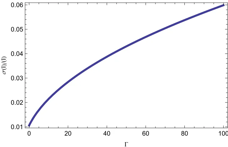
3.1 Theoretical standard deviation during early growth in a large population . . 34

3.2 Configuration model: Multiple link adjustment . . . 36

3.3 Configuration model: Self-link adjustment . . . 37

3.4 Standard deviation during early growth; theory and simulation . . . 39

4.1 Change inR0 and final size due to✏ . . . 47

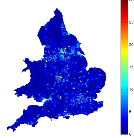
4.2 Number of workplaces with a high number of employees, showing concen-tration in main urban areas. . . 49

4.3 Final size of an epidemic where we alter ✏ and N. Even a small change from ✏= 0 to✏= 0.01 can give a significant increase in the final size of the epidemic. . . 50

4.4 Number of workplaces containing between 1 and 100 employees. . . 51

4.5 Binnings of workplace size distribution . . . 53

4.6 Comparsion of Blue Sheep and ONS Business data . . . 54

4.7 Total number of infections in workplaces by✏ . . . 56

4.8 O↵set truncated power law fit; binning 1 . . . 61

4.9 O↵set truncated power law fit; binning 2 . . . 62

4.10 Total number of workplace infected by ✏; o↵set truncate power law . . . 62

4.11 Likelihood fit workplace data from sizes 100–7500 . . . 63

4.12 Workplace data compared to likelihood and minimum cdf error fits to o↵set truncated power law for xmin = 100, binning 1 . . . 64

4.13 Workplace data compared to likelihood and minimum cdf error fits to o↵set truncated power law for xmin = 100, dinning 2 . . . 65

4.14 Total number of workplace infected by ✏; o↵set truncate power law fitted forxmin = 100 . . . 65

4.15 Discrete power law fit; binning 1 . . . 67

4.16 Discrete power law fit; binning 2 . . . 68

4.17 Total number of workplace infected by ✏; discrete power law . . . 69

4.18 Workplace data compared to likelihood and minimum cdf error fits to dis-crete power law forxmin= 1,4,50,500 and 1500, first binning . . . 70

4.19 Workplace data compared to likelihood and minimum cdf error fits to dis-crete power law forxmin= 1,4,49,499 and 1499, binning 2 . . . 71

4.20 Total number of workplace infected by ✏ for both binnings; discrete power law for various values ofxmin . . . 71

4.21 Log-normal distribution fit; binning 1 . . . 73

4.22 Log-normal distribution fit; binning 2 . . . 74

(6)

4.24 Comparison of attack rates; workplace data, fitted power law distribution

and households . . . 81

5.1 Visualisation of data sources used in construction of the synthetic popula-tion. . . 95

5.2 Central London workplaces and retail locations . . . 100

5.3 Workplaces and retail locations around Oxford Street, London . . . 101

5.4 Contact structures for synthetic population and POLYMOD . . . 105

5.5 Impact of activity type on number of contacts and survival function; syn-thetic population, Social Contact Survey and POLYMOD . . . 106

5.6 Clustering in synthetic population compared with Social Contact Survey . . 107

6.1 ISIS simulations (i) . . . 110

6.2 ISIS simulations (ii) . . . 111

6.3 ISIS simulations (iii) . . . 112

6.4 ISIS simulations (iv) . . . 113

6.5 Degree distributions for synthetic population, contact survey and POLYMOD115 6.6 Pairwise approximations of epidemics on three degree distributions . . . 117

6.7 Predicted impact of work closure on R₁, pairwise theory ODEs . . . 118

6.8 WAIFW simulations (i) . . . 124

6.9 WAIFW simulations (ii) . . . 125

6.10 Meta-population simulations(i) . . . 131

6.11 Example of two clustered networks . . . 132

(7)

Acknowledgments

The research detailed in this thesis was funded by the Engineering and Physical Sciences Research Council (EPSRC) via the Complexity Science Doctoral Training Centre at the University of Warwick. Additionally two visits were made to the Network Dynamics and Simulation Science Laboratory at Virginia Tech, which was made possible by funding supplied by this hospitable and helpful group.

During my time of study at Warwick many people have provided me with support. First and foremost is my supervisor for this work, Thomas House, who has a seemingly

inex-haustible well of both knowledge and patience. I also thank the sta↵ and administration

of the Complexity Science DTC for their help in all matters, and the WIDER group at Warwick for interesting discussion.

I was privileged to be surrounded by many generous, interesting and friendly people in this department who increased my enjoyment of research considerably. These include, Peter Dawson, Chris Oates, Ben Collyer, Anthony Woolcock, Sergio Morales, Anas Rana, Ellen Webborn, Marcus Ong, Dan Sprague, Mike Irvine, Yu-Xi Chau, Davide Michieletto, Dario Papavassiliou and Tom Machon. I thank Anthony Woolcock and Adrienne Davies, Ben Collyer and Marcus Ong, Peter Dawson and Jen Lawson along with Chris and Lucy Oates for their hospitality on numerous occasions and Davide Michieletto, Tom Machon, Anthony Woolcock, James Porter, Peter Dawson and Chris Oates for helping me hone my squash skills and to a much lesser extent my tennis skills. I also owe a large debt of gratitude to Justin Lessler for employment over the last few months of my PhD write-up.

(8)

Declarations

Parts of this thesis have been published elsewhere:

• M Graham & T House (2012), ”Dynamics of stochastic epidemics on heterogeneous

networks”. J. Math. Biol.

The presented thesis is MG’s own work, except where research involving collaboration is

concerned. In these circumstances, MG’s contributions are indicated. This theses has not

(9)

Abstract

Contact structure between individuals in a population has a large impact on the spread of an epidemic within this population. Many techniques and models are used to investigate this, from heterogeneous age-age mixing matrices to the use of network models in order to quantify the heterogeneity in the populations contacts.

For many diseases, the probability of infection per contact, along with the exact

con-tact structure are unknown, compounding the difficulty of identifying accurate contact

structures.

In this thesis, the impact that the contact structure has on the epidemic is examined in

several di↵erent ways. Analytical expressions for the variance in the spread of an epidemic

in its early exponential growth phase on heterogeneous networks are derived, showing that the third moment of the degree distribution is needed to fully specify this variance. This quantifies the impact that very well connected individuals can have on the early spread of an epidemic through a network.

The dependency of the potential epidemic on the heterogeneity in workplace sizes and transmission rates is examined. It is shown that large workplaces can increase the expected

size of the epidemic significantly, along with increasing the e↵ectiveness of control strategies

enacted during the early stages of an epidemic.

In addition to this, a synthetic population is constructed for England and Wales from available datasets, in an attempt to model the spread of an epidemic through a realistic network of comparable size to the true population. The contact structure that is derived from this is compared with that taken from two surveys of contact structure in the same

population, using simple models, and qualitative di↵erences are seen to exist between the

(10)

Chapter 1

Introduction

Since the work of Kermack and McKendrick [Kermack and McKendrick, 1927], the study of epidemics using mathematical modelling has become widespread. One of the most prominently studied models is of a disease which has three compartments or classes which

individuals can pass through, namely: a susceptible class, S, containing those individuals

who can contract the disease; the infectious class, I, who currently have the disease and

can transmit it to those in the susceptible class; and the removed, R, which contains

those who have previously contracted the infection and have now been removed from the dynamics of the epidemic, be that by recovery to immunity from the infection or by death.

This type of model is often referred to as theSIRmodel for obvious reasons.

Following this example, a large amount of study of epidemics via the use of mean-field dynamics has been undertaken [Anderson and May, 1992]. For the mean-field dynamics, a key assumption is that all members of the population have equal probability of spreading an epidemic to any other member of the population at all times. Though a very useful assumption, in reality this is not what is observed, and the heterogeneity that is present in the contact structures of populations has a large impact on the spread of an epidemic [Keeling, 2005; Rohani et al., 2010] and has become the subject of numerous survey studies [Read et al., 2008; Mossong et al., 2008; Danon et al., 2012; Read et al., 2011, 2014]. Additionally, methods to infer contact structures through phylogenetic analysis of disease strains in populations have recently been developed [Volz et al., 2009; Leventhal et al., 2012; Frost and Volz, 2013].

The theme of heterogeneity in contact structure is the main focus of this thesis. In _§3,

the variance of early growth period of an epidemic on a heterogeneous network is consid-ered. To investigate this, the neighbourhoods of susceptible and infected individuals are considered, and the epidemic is shown to be density dependent. The work of Kurtz [1970, 1971] relating to density dependent processes is then used to calculate the variance of the number of infected individuals during the early growth period. The theoretical expression that is derived is then compared with that seen from simulating epidemics on networks and a good agreement between the two is seen.

In §4 data detailing the workplace size distribution of the UK is considered. Workplaces

are where a lot of heterogeneity in the number of contacts that people have is generated, as the number of contacts made in the home or in schools show much less variance than the workplace. How this distribution, coupled with transmission rates which are modified

(11)

spread of an epidemic is examined. This is achieved by fitting several di↵erent distributions to fit the workplace size distribution, which are then combined with the transmission rates along with the standard final size equation in a mean-field model to estimate the potential epidemics size for these fitted distributions. The overall and secondary attack rates, which give the overall proportion of at risk individuals who become infected, and the proportion of these infected by the initial infected respectively are also considered for the modified transmission rates. It is shown that for large workplaces sizes, the increased presence of which increase the predicted final size of the epidemic, coincide with the lowest secondary attack rates. This has implications for possible control methods, as many infections can be averted by acting early in this scenario.

In _§5 the construction of a synthetic population, whose contact network represents

Eng-land and Wales is described. This is a network model which has the same number of individuals as there are in England and Wales, which is constructed to align with several statistics taken from census data. There have been several similar studies in the last few years which have focused on the USA [Eubank et al., 2004] and Italy [Iozzi et al., 2010].

This involves bringing together many di↵erent data sources, such as census data, and

di-ary style information to attempt to create a representative contact network for England

and Wales. Once constructed, this can be used to compare the efficacy of possible

in-tervention strategies on a national scale. Various measures of this synthetic populations contact structure are then compared with two contact structures derived from surveying the population of Great Britain. These two surveys are POLYMOD [Mossong et al., 2008] and the UK contact survey [Danon et al., 2012].

Finally in _§6, simulations conducted using the synthetic population are compared with

simulations using simpler models (pairwise approximation, who-acquires-infection-from-whom and meta-population models), where the contact structure is defined by data gath-ered from the synthetic population, along with POLYMOD and the UK contact survey.

This is in order to quantify how di↵erent these contact structures are, along with what is

gained by including so much detail in the full synthetic population.

Firstly in _§2, we introduce basic ideas behind mathematical models of infectious disease

spread, from deterministic mean-field models up to stochastic heterogeneous network

mod-els. This leads into _§3 which involves theory of stochastic heterogeneous network models.

(12)

Chapter 2

Background

2.1 General modelling techniques

The use of mathematical models to aid in understanding the spread of infectious diseases began in the 18th Century [Bernoulli, 1766], and has become an important tool in the study and prevention of epidemics. The beginnings of modern mathematical modelling of diseases can be seen to have begun with Kermack and McKendrick [1927]. Since this early investigation, there has been much study of epidemic models and they now take a variety of mathematical forms [Anderson and May, 1992; Keeling and Rohani, 2008], and are routinely used to inform policy on disease control and contribute towards public health plans [Ferguson et al., 2003; Riley et al., 2003; Tildesley et al., 2006; Baguelin et al., 2010].

The most popular modelling approach is to generate a set of di↵erential equations which

describe the infection process for a population, and then examine what the consequences of this model are. Individuals in the population are put into separate ‘compartments’, which describe the state of the infection within the individual in question. A member of the population will begin in a ‘susceptible’ state, and once exposed to infection will progress

through a number of di↵erent compartments as time progresses. The most prominent

example of this is the susceptible-infectious-removed (SIR) model, first formulated in

Kermack and McKendrick [1927] and since described in Dietz [1967], Keeling and Rohani [2008], Bailey [1975] and many other texts.

In this model, at any point in time everyone is either susceptible to the disease, infectious with it, or removed from the future disease dynamics. This model is obviously a simplifi-cation of reality, but provides a useful starting point for modelling diseases where previous infection confers long-lasting immunity, for example outbreaks of childhood diseases like measles, some respiratory illnesses like pandemic influenza, and historical pathogens such as smallpox [Keeling and Rohani, 2008]. It is often assumed that the time scales of the infection and the epidemic are such that the population size will be the unaltered through-out the epidemic, with the exception of death caused by the infection, i.e. births and death by other causes are irrelevant.

(13)

an equal probability of contracting the infection at any given time, and that they can be infected by any infectious member of the population, meaning that members of the population are interchangeable. For the simplest, deterministic, form of this model, the

governing di↵erential equations are given by the following:

dS

dt = SI

dI

dt = SI I

dR

dt = I ,

(2.1)

whereS,IandRare the proportion of individuals in the susceptible, infected and removed

compartments respectively, S +I+R = 1, is the removal rate of infected individuals

and I is the rate at which the infection is passed on to each susceptible. This is an

example of ‘frequency dependent’ transmission, as as the population size increases, the number of individuals infected by a randomly chosen individual will not increase. As we

have S+I +R = 1, we can in practice work simply with equations for S and I, as the

value of R will be defined by this relationship.

To see an increase in the number of infected individuals we require that dI/dt > 0,

which implies that / >1/S. If we begin in an entirely susceptible population, then we

require that / >1 in order to see an epidemic in the population. This number ( / )

is referred to as the basic reproduction number and is denoted by R0. This is equal to

the average number of people that a typical individual infects in an entirely susceptible population.

There are many ways in which this simple model can be amended to reflect reality more closely. The transmission rates are time independent, which implies that it is equally likely to that you will transmit an infection to someone else at all points of your own infection, which is not what is seen in reality [Hall et al., 1979; Lee et al., 2009]. Some infections, such as influenza, are also known to be seasonal, meaning that the probability of infection will increase or decrease depending on the time of year. The assumption of just three compartments is also often questionable, as it is unlikely that at the moment of infection, an individual will become infectious themselves, implying that the addition of a latent infected class is desirable. There is a great deal of work also using this

susceptible-exposed-infectious-removed (SEIR) model e.g. Hethcote and Tudor [1980]; Longini [1986];

Li and Muldowney [1995]; Li et al. [1999] amongst many others.

The advantage of using models with additional compartments is that more complex disease dynamics can be included in the model, along with the ability to examine increasingly

complex interventions. For example using an SEIR model and modelling the impact of

separating infected individuals from a proportion of their contacts, an individual in the exposed class can be allowed to transmit the disease to their contacts at a lower rate than those who are infectious, but will not be identified as infectious and therefore will not be separated from any of their contacts. In theory any number of compartments can be added

to the model to describe di↵erent states of the disease that individuals are in along with

age specific compartments. However, doing this increases the difficulty of parameterising

these models and interpreting their output.

(14)

is not what we would expect to observe in reality, as there are many occasions during a

real epidemic where chance events occur, resulting in a di↵erent pattern of disease spread.

Along with this, for (2.1), if the valueR0 = / >1, we will observe an epidemic, which

will infect a significant fraction of the population, whilst ifR0 <1, then this will not occur. Again this is not what we would expect to see on all occasions, as supercritical epidemics

can die out, and those with values ofR0 <1 can infect a significant number of people. If a

population is very large, then it is reasonable to expect that the final number of infections would be similar if we could repeat the whole epidemic process with no additional control interventions, as all random events get averaged out to impart no significant impact on the spread of the disease. However if we consider smaller populations, the random events will have a much greater impact on the final outcome [Bartlett, 1957; Lloyd, 2004; Britton, 2010]. Therefore the use of stochastic models is common place, which allow us to examine the role that the uncertainty inherent in any epidemic has. The disadvantage of using

such models is the increase in difficulty of extracting meaningful statistics from them due

to this unpredictability.

One of the first stochastic models for epidemics is the Reed-Frost model [Wilson and Burke, 1942; Abbey, 1952; Bailey, 1975], which takes place in discrete time, to describe

an epidemic spreading through a population. Again this falls into an SIR type model,

where individuals are infectious for one time step, before being removed. Here the number of susceptible individuals during the next time step is given by a binomial distribution;

S(t+ 1) = Bin(S(t), qI(t)), where q is the probability of contact between any susceptible-infectious pair in the population. Hence the model is sometimes referred to as a ‘chain

binomial model’, as we are e↵ectively picking from a chain of binomial distributions. The

number of infectious individuals at timet+1 is then given byI(t+1) =S(t) S(t+1).

For a simple stochasticSIR continuous time epidemic, we again haveS(t),I(t) andR(t)

denoting the number of susceptible, infected and removed members of the population at

time t, but these are now random variables. In much research on stochastic epidemics,

the length of a infection of an individual until removal is assumed to be exponentially

distributed, with removal rate per unit time (equivalent to removal being a Poisson

process with rate ). Contacts between members of the population also take place at the

points of a Poisson process with rate /N, where N is the population size. This choice

of infection length results in the epidemic process _{(S(t), I(t), R(t)) : t > 0_} having the Markov property [Bailey, 1975], as the next event to take place, be that an infection or a recovery, depends only on the current state, and not the history of infections.

A common technique for investigating stochastic models is to explicitly realise numerous stochastic trajectories which are defined by the dynamics of the epidemic [House et al., 2012]. There are many methods that are used to do this including Sellke’s construction [Sellke, 1983] and Gillespie’s algorithm [Gillespie, 1977], which both give results equiva-lent to the stochastic model. Alternatively, the tau-leap method [Gillespie, 2001] gives an approximation to the stochastic model, but is appreciably faster than the Gillespie algo-rithm. In practice, many simulations are performed, from which it is possible to extract statistics such as the expected number of infections or the variance possible in the size of the epidemic at any point in time.

Along with this, there are several analytical methods which are used to describe stochastic

models. One example is di↵usion approximations, which examine the fluctuations from

the deterministic trajectory which the stochastic epidemic converges to as the population

(15)

describe the stochastic fluctuations around this deterministic limit [Clancy et al., 2001;

Ross, 2006; Dangerfield et al., 2009; N˚asell, 2002]. This work is based on the technical

results derived by Kurtz [1970, 1971] and described again by Ethier and Kurtz [1986], Andersson and Britton [2000] and many other texts.

Another analytical method for examining this particular epidemic is that of directly con-sidering the master equation (also called Kolmogorov forward equations) of the Markov

process which governs the probability of seeing a particular state for psi(t) = P(S(t) =

s, I(t) =i) [Keeling and Ross, 2008; N˚asell, 2002]. This allows us to analyse the

proba-bility of any possible state occurring with one model realisation per parameter set, whilst with Monte Carlo simulation, this requires a large number of realisations to achieve. This

method requires the use of di↵erential equations to describe all possible states of the

epidemic, which is 1₂(N+ 1)(N + 2). Therefore as the population size increases, the

com-putational cost of this method becomes infeasible, meaning that it is quicker to simulate the epidemic multiple times directly via Gillespie’s algorithm or an equivalent approach, and draw from these simulations, conclusions about the probabilities.

Stochastic moment-closure models are also used to describe the behaviour of the epidemic

by taking the moments of the di↵erential equations describing the epidemics [Isham, 1995;

Herbert and Isham, 2000; Krishnarajah et al., 2005; Keeling, 2000; N˚asell, 2003; Keeling

and Rohani, 2008]. For example we can calculate the mean, variance and higher moments

of the number of infective individuals in the population at timetusing this method. This

method allows us to, in theory, describe the behaviour of an infinite number of simulations,

but, in practice, it is made difficult by the need to increase the number of moments to

exactly describe the system at any given level. For example the second moment is needed to describe the evolution of the first moment, and the third moment is needed to describe the second. Therefore it is often the case that any moment above the second is set to zero, or at a certain level, the moment is approximated by a combination of lower moments. This is a great advantage over deterministic models, as these essentially follow this process, but set any moment above the first to zero. Again, however, it is often preferable to directly simulate a number of realisations, with the necessary number of simulations increasing as the order of the moment increases.

The addition of stochasticity is one step towards reality. However the assumption that all members of the population are equally likely to come into contact any other member of the population is still used in the models described so far. In many populations, not all contacts that are made are made at random, for example in human populations many interactions which would be described as contact take place in the home or at work. Network models do not make this assumption.

2.2 Network models

The use of networks as a generalisation from homogeneous mixing is becoming one of the most widely used in epidemiological modelling. Contact between two individuals of the population we are considering forms a link between them. Once a link is established, the infection can be passed along it in either direction. Specifically what contact is depends on

the disease, i.e. it is di↵erent for a respiratory infection compared to a sexually transmitted

infection. There have been many examples of using networks to study the spread of disease

(16)

approaches to network modelling.

A network can be described by anN_⇥N matrixA, which is called the adjacency matrix.

The matrix will be symmetric if the network is undirected, meaning that if node i has

node j as a contact, then node j has node i as a contact. If the network is unweighted,

ı.e. all links are of equal strength, then the entries of A will be binary, where the entry

Ai,j will be 1 if nodes i and j have a link between them and 0 otherwise. For weighted

networks, entryAi,j gives the strength of contact between nodesiandj, which can signify,

for example, the length of time whichiand jspend together. The degree of a node is the

number of contacts that it has in the network. The degree of node iis denoted ki and is

given byki=PjAij.

In this context, a network gives the set of contacts made by all members of the population in question, with whom it is possible to receive or transmit an infection. Some of the earliest uses of networks in this way detailed the spread of sexually transmitted diseases e.g. Klovdahl [1985]; May and Anderson [1987]. Such diseases are ideal for study using networks due to the well defined mechanisms required for transmission to occur, unlike with many other diseases where short-lived interactions can result in transmissions, for example with measles [Paunio et al., 1998] or respiratory infections like influenza.

In the network, a pair is two nodesiand j, who are neighbours of each other. A triple is

given by three nodesi,j and l, whereiand j are neighbours and j and lare neighbours.

Ifiand l are also neighbours, then this triple forms a triangle in the network.

Bearing this in mind, the progression of an epidemic on a pre-specified network avoids the problem of how to reconstruct a contact network. In this scenario the epidemic will take place on a predefined or static network, or one which is evolving as defined by a set of given rules.

2.2.1 Network properties and impact on disease spread

There are several generic properties of networks, each of which can have an impact on the spread of a disease through the network.

2.2.2 Degree distribution

The degree distribution of a network is the distribution of the number of neighbours

that the nodes in the network have. This is defined by a function P(k), which gives

the probability that a node selected uniformly at random will have k neighbours. It is

clear that the higher the degree of a given node, the more likely it is to become infected during an epidemic, and it is also more likely to spread the infection once it has become infected. It has also been shown, that as the population size diverges, that if there is a large variance in the degree distribution, such as in a scale-free network then the infection can spread very quickly through the network [Barth´elemy et al., 2004], and if the variance is also divergent, then there will be no epidemic threshold in the network, meaning that no matter what the ratio between removal and transmission rates, the disease will always

infect a non-zero proportion of the population [Bogu˜n´a et al., 2003; Pastor-Satorras and

(17)

In more realistic networks however this increase in variance of degree distribution can help to control the spread, since if the individuals who have many more than the average number of contacts, termed “super spreaders”, can be identified and removed from the

dynamics, then this can be much more e↵ective than random control methods

[Lloyd-Smith et al., 2005; Meyers et al., 2005] and even prevent large outbreaks from occurring [Cr´epey et al., 2006]. In the case of sexually transmitted diseases or injecting drug users, it is more realistic to expect that these people can be identified and attempts can be made to remove them from the dynamics [Magiorkinis et al., 2013].

Along with super-spreaders, who have a large number of contacts, for diseases which are spread through contaminated droplets, such as SARS and influenza “super-spreading events” have been observed, which environmental conditions can be responsible for [Riley et al., 2003; Galvani and May, 2005; Lipsitch et al., 2003]. These events are unpredictable,

which makes preventing them difficult, but we can model them by including more people

with greater numbers of contacts if we desire.

In reality the exact network upon which a disease spreads is unknown, and in many cases, such as respiratory diseases in humans, essentially unknowable. However without assuming something about the contact network we are unable to progress at all. There have been many attempts made to characterise contact patterns, for example Mossong et al. [2008], Liljeros et al. [2001] and Danon et al. [2012], which lend weight to the opinion that there is a heavy tail in the distribution of the number of contacts that people have. This means that in general it is not expected that the distribution of number of contacts would be Gaussian or binomial, but is more likely to be negative binomial or power law distribution.

2.2.3 Clustering

The level of clustering in the model gives us the probability that two contacts of a randomly

chosen individual are contacts of each other. It is often denoted by . If the level of

clustering in our model is 0, then the probability of two of my contacts contacting each other is 0, whilst if it is 1, then it is certain that they will be contacts of each other. Informally, this is equal to 3 times the number of triangles in the network, divided by the total number of triples in the network. To calculate it for a given network we perform the following calculation,

= P

i,j,kAijAjkAki

P

i,j,k6=iAijAjk

. (2.2)

An increase in clustering will reduce the extent to which an infection will spread [Watts and Strogatz, 1998; Eames and Keeling, 2003; Kiss et al., 2005; House and Keeling, 2011a] along with increasing the time to reach the peak of the epidemic [House and Keeling, 2011a]. This is due to the fact that for the infection to spread, it is necessary for an infected individual to have susceptible contacts. Additionally, it is obvious that to become infected in the first place, one of your contacts must have been infected before you. Therefore in a highly clustered network, the probability of having a large number of susceptible contacts rapidly decreases as the epidemic progresses, since to get infected in the first place, a number of your own neighbours are likely to have been infected before you. In contrast, in a network with low or no clustering, the depletion of susceptible contacts that an infected

(18)

also neighbours of the infected you, or the node which infected that node and so on, and are therefore less likely to have picked up the infection previously.

In terms of combating a particular infection, contact tracing is a common tool for control-ling and assessing the spread of an epidemic. This is the practice of tracing the contacts which were made by an infectious individual, as the likelihood that this will lead to an infected individual is greater than choosing from the population at random. Once traced, these contacts can be quarantined if necessary, or in the case of animal diseases, where farms are taken to be nodes rather than individual animals, the farms can be prevented

from further export or import of animals and cordoned o↵. This has been seen to be

successful in identifying infected individuals for sexually transmitted diseases [G¨otz et al.,

2005; Fish et al., 1989] and it was somewhat successful when used in Great Britain during the spread of foot-and-mouth disease in 2001 [Ferguson et al., 2001a,b] and the SARS outbreak of 2002-03 [Lipsitch et al., 2003].

This can be e↵ectively incorporated into a network model; contacts of infected nodes can

be identified, with a certain efficacy, and then quarantined if infected. This contact tracing

is usually accompanied by a specified efficacy within a model, as in reality it is unlikely

that for certain disease types, all contacts will be found. It has been shown [Eames and Keeling, 2003; Kiss et al., 2005; House and Keeling, 2010], that as clustering increases, the

levels of efficacy needed to produce a given reduction in disease spread decreases. Again

this is because a randomly selected, infectious node is likely to have a greater number of infectious contacts in a highly clustered network than in a network with no clustering, meaning that the average number of infectious individuals found each time contact tracing

is performed will be higher. However, as efficacy increases towards 1 this result is reversed

[House and Keeling, 2010], which demonstrates how complicated and subtle the interaction of clustering and the spread of the epidemic is.

In reality, we may expect that the level of clustering will be non-zero and a survey of the UK population [Danon et al., 2012] which had over 5,000 responses reports the level of clustering in the population as being as high as 0.38.

2.2.4 Degree assortativity

A degree assortative network is one in which the high degree nodes are contacts of other high degree nodes and low degree nodes are neighbours of low degree nodes more than would be expected at random. A degree disassortative network has nodes with high and low degree as neighbours more commonly than would be expected at random. This is often

denoted byr. To calculate this for a given network, the following is calculated,

r=

P

j,kjk(ejk qjqk)

P

kk2qk (Pkkqk)2

, (2.3)

where qk = (kP+1)pk+1

jjpj , which is referred to as the remaining degree, and ejk is the joint

probability distribution of the remaining degrees of the nodes at either end of a randomly chosen edge [Newman, 2002b]. This lies between -1 and 1, which define a perfectly disas-sortative and asdisas-sortative network respectively.

(19)

connected component of the network. In a network with a divergent number of nodes, if the largest connected component is a non-zero fraction of the total network size, then this is referred to as the giant component of the network. It was shown in Newman [2002b], that all other things being equal, the probability that a giant component exists is greater for an assortative network than for a random network, and that in turn the probability is greater for a random network than for a disassortative network. This suggests that

combating disease on assortative networks can be more difficult than other networks, due

to the fact that high degree nodes are connected to each other, removing these nodes will

be redundant until a high proportion of them are removed. This increases the difficulty

of combating the spread of diseases where the networks are assortative, as is the case for sexual activity, compounding the impact of many sexually transmitted diseases [Potterat et al., 1985; Granath et al., 1991], along with the practice of needle sharing and the number of injecting partners in injecting drug users [Mills et al., 2012].

The opposite is true for disassortative networks in that they can be easily broken up by removing the high degree nodes. This means that these types of networks are especially vulnerable to targeted attacks and as many networks which are considered valuable, such as the internet and food webs are disassortative [Martinez, 1991; Zhang et al., 2012], these may be more vulnerable than anticipated. In terms of disease control, a disease transmit-ting on a disassortative network, may be more readily controlled if the high degree nodes can be identified and removed, though in practice this would not be straightforward.

An example of a disassortative network is given in Kiss et al. [2006a], where the di↵erence

between a network describing sheep movements which was derived from data regarding movements within the UK is compared to a randomly constructed network of the same size and degree. The nodes of these networks are all places which sheep move to and from, so include sheep markets along with farms. These data driven networks are disassortative, meaning that nodes with many connections are more likely to contact nodes with lower degree. This is due to the fact that the most likely route of movement is from a sheep market to any number of farms, which results in the market having a higher degree than the farms to which sheep travel.

This comparison shows that the proportion of nodes which become infected is higher for random networks. This can be explained by the disassortativity of the data driven networks, as the linking of high degree nodes with low degree ones implies that it may take longer on average to reach highly connected nodes in the network, and from there will transmit infection to nodes with lower than expected degree, slowing the spread of the epidemic. Additionally these data derived networks also have a longer path length than the randomly constructed networks, the impact of which is discussed below.

2.2.5 Average shortest path length

Path length (or shortest path length) in a network is the number of steps required to get from one node to another. The average shortest path length is the average of this number over all pairs of nodes which comprise the network. This is defined per connected

component, since otherwise we would get1for all networks which are not fully connected.

(20)

shortest path length increases, the speed of spread of the epidemic will be decreased and the rate of spatial spread will also decrease [Watts and Strogatz, 1998].

To move away from the mean-field assumption, a simple way to introduce some structure into our model is to consider the spread of an epidemic on a lattice [Sato et al., 1994]. Here contacts are defined to be the neighbours of each node on the lattice. This a realistic assumption to make in certain populations, such as in the spread of fungal parasites from plant to plant [Otten et al., 2004], but for animal and human populations this is often not a close approximation of reality. This can be extended to lattices of more than one

dimension and also include links to k nearest neighbours, rather than simply immediate

neighbours.

As the lattice has connections only between nearest neighbours (or some numberknearest

neighbours) the average shortest path lengths will be high. For example to get from one end of the lattice to the other, an infection must pass through every connecting node.

To avoid this problem the lattice can be re-wired by removing links between certain neigh-bours, and attaching to a randomly chosen node in the network. This will significantly decrease these large path lengths which occur. This was popularised by Watts and Stro-gatz [1998], and these networks were known as ‘small-world’ networks, due to the fact that as the path lengths were significantly shortened, there were far fewer nodes needed to be passed through in order to reach anyone in the population. This explains the ‘small-world’ problem examined by Milgram [Milgram, 1967] which gave rise to the notion of six degrees of separation, as if this is assumed to be representative of the human population, any one person could then reach any other person, by going through (for arguments sake) six or fewer intermediaries.

2.2.6 Models and modelling techniques

Having discussed the properties of networks that impact on disease spread, we will now

discuss di↵erent network models and techniques used to investigate disease spread on

networks.

The first step away from mean-field mixing, where everyone in the population is able to

contact everyone else, is where every individual in the population has a given number n

contacts. These types of networks are called regular networks. The spread of an epidemic on these networks have been compared to the mean-field models [Keeling, 2005] and the

impact of small-world e↵ects [Santos et al., 2005]. As noted previously, regularity is a

reasonable assumption for certain populations for [Otten et al., 2004], however for networks of human interaction, this is a poor assumption Wadsworth et al. [1993]; Liljeros et al. [2001]; Mossong et al. [2008]; Danon et al. [2012].

Heterogeneity in the number of contacts that individuals have is included in many network

models. For example in Erd¨os-R´enyi (ER) random graphs the link between every pair of

nodes is present with a given probabilityp. For our purposes, when the construction of a

network is needed, the configuration model [Molloy and Reed, 1995] is used to construct the network from the degree distribution.

(21)

epidemic has been calculated [Keeling, 1999; Diekmann and Heesterbeek, 2000].

In most cases, the network upon which either theoretical or simulation based investigation of epidemics is performed are static networks, fixed at the starting point of the epidemic e.g. Newman [2002a], Volz [2008] and Mossong et al. [2008] to name a few. However there are also examples where this network is allowed to evolve over time, interacting with the spread of the epidemic e.g. Kamp [2010], Miller and Volz [2012] and Pastor-Satorras and Vespignani [2001]. In the case of Pastor-Satorras and Vespignani [2001] along with May and Lloyd [2001] and some models of Miller and Volz [2012] the network of contacts is changing constantly. In reality, the contact network for a respiratory infection will have some links which are always present (made often or daily), and some which are more short lived, such as those made whilst using public transport. This has been considered by including a ‘global’ infection term [Kiss et al., 2006b; Ball and Neal, 2008], which allows the disease to be passed between members of the population that do not have more than one interaction.

Similar techniques to those developed for stochastic mean-field models have been used for investigating stochastic network models, with moment-closure methods e.g. Taylor et al. [2012], Rand [1999] and Rogers [2011] along with Kolmogorov-forward equation techniques [Allen et al., 2008; Simon et al., 2011].

Additionally, we note the use of a probability generating function method [Volz, 2008; Miller, 2010], which allows us to succinctly denote properties of the network which influence the dynamics, to derive a small number of nonlinear ODEs that describe the dynamics of an SIR infection on a random heterogeneous network.

In general to consider the dynamics of the epidemic in continuous time, a Markov chain

model is used. For an SIR-type epidemic model on an arbitrary graph with N nodes,

Markov chain would involve 3N _{ODEs, which quickly becomes computationally intractable.}

The method proposed by Ball and Neal [2008] involves creating a configuration model

network at the same time as the epidemic tree, which can be defined by 2M ODEs in the

deterministic large N limit, where M is the maximum number of contacts that any one

node has.

By making an assumption about the neighbourhoods of individuals on the network a far smaller equation set has been derived [Volz, 2008]. A sophisticated convergence proof [Decreusefond et al., 2012] has demonstrated the exactness of this assumption, and hence

the equation set, in the largeN limit.

To investigate the inherent stochasticity of epidemics without a large increase in

dimen-sionality has led researchers to consider the di↵usion limit. This general approach to

stochastic processes is typically either attributed to N G van Kampen [1992] or Kurtz [1970, 1971]. Here the stochastic Markov model can be approximated by a set of determin-istic ODEs, with the stochasticity being characterised by scaled white noise processes with magnitudes defined by the transition rates between the states of the Markov model.

Such methods have been used to derive a low dimensional model in which properties of the noise in a stochastic epidemic model can be investigated analytically [Alonso et al., 2007; Black et al., 2009], by Ross [2006] to obtain expressions for the mean and variance of a

meta-populations model, and by Colizza et al. [2006] to model the e↵ect of air travel on the

(22)

(23)

Chapter 3

Early growth variance of epidemics

on heterogeneous networks

In this chapter we will apply the results of Kurtz [1970, 1971] to SIR-type epidemic dynam-ics on a configuration model network, as was done for SIS dynamdynam-ics on a regular graph by Dangerfield et al. [2009]. Using this we obtain a four-dimensional set of stochastic ODEs, from which we derive an analytical expression for the variance of the asymptotic early growth of an epidemic on a network given its degree distribution. We simulate epidemics on various networks to confirm the utility of our analytical results.

3.1 Model description

The following sections are an extended look at the results published in Graham and House [2013]. Firstly we discuss the construction of a network model and the limitations of using network models in the way that we have used them.

There areN individuals connected to each other on a configuration model network. This

implies that there is no clustering in the population and so there are no short loops in the population. This means that the consideration of depletion of susceptible contacts is

made simpler due as we can be sure that when an individualiis infected by individualj,

that the neighbors ofiwill not have been infected by individualj.

Individuals are compartmentalised by their disease state S, I, or R, and their number

of neighbours on the network, their degree, k.Individuals of type Sk become Ik at a rate

equal to the product of the transmission rate⌧ and their number of infectious neighbours.

Individuals of typeIk become Rk at a rate .

As the aim of this work is to get a theoretical result using di↵usion methods, I am interested

in the largeN regime, in which [Sk] denotes the expected number of susceptibles of degree

k, [Ik] the expected number of infectious individuals of degreek, and [AB] for the number

of connected pairs of individuals on the network where one is typeAand the other is type

B. Omission of a subscript denotes implicit summation, e.g. [S] =P_k[Sk]. Proportions

of the population who are, say, susceptible and of degreekare represented by the bracket

(24)

For the di↵usion limit, the population size N is allowed to increase towards ₁, whilst

keeping the proportions of susceptibles and infecteds of di↵erent degrees constant. What

follows is a description of the deterministic process that the epidemic approaches when the process can be described as ‘density-dependent’. Using appropriate theory [Kurtz, 1970, 1971], the stochasticity of the system can be characterised, and used to calculate the variance of the epidemic during its early growth phase.

Limitations of this approach are now considered.

3.1.1 Limitations of network models

The main limitation of network models is that the true network on which an epidemic will take place is unknown. Using a degree distribution to describe a full contact network is limited and considering an unweighted network means that much subtlety is lost in the description of the contact structure of a population.

As mentioned previously, the network is assumed to be unclustered, which is known to be a poor assumption [Liljeros et al., 2001; Danon et al., 2012]. Additionally, this has a

significant impact on the dynamics of an epidemic as described in _§2.2.3.

It is also assumed that the network upon which the epidemic is spread is a static network, meaning that the network is the same every day, which is again unrealistic.

Next notation and some standard approaches to the SIR on a network are described.

3.1.2 Notation, mean field and pairwise models

The degree distribution is given by P(k) as is noted above, and dk is used to denote the

proportion of nodes which have degree k. N dk gives the number of nodes which have

degree k. Also of use to the analysis of this system is the probability generating function

(pgf) of the degree distribution. This is denoted by g(x) and g(x) = Pdkxk. Note that

this gives a simple way of expressing many aspects of the system, e.g. g0(1) =Pkdk= ¯n

where ¯nis the mean of the degree distribution.

Another assumption about the system is that for susceptible nodes, infection across each link is independent of all other links that the node in question has. The implication of this, is that if we calculate the probability that a node with one link which is selected

uniformly at random, conditioned on having only 1 link, is susceptible at timet, and label

this ✓, then the probability that a node of degreek is susceptible at timetis given by✓k.

If there are no nodes of degree 1, or if we were considering a complete graph or a regular network, then we can think of this value as being the probability that infection will have passed down a specific link.

Using this variable, it is clear that ✓= [S1]/N d1 and that [Sk] = N dk✓k. This therefore

also gives that [Sk] = N dk([S1]/N dk)k. Using the pgf allows us to express [S] as, [S] =

P

[Sk] =PN dk✓k=N g(✓). It follows that instead of writing down equations that allow

[S] to be tracked, ✓ can be used in its place.

The progress of the epidemic can be described by a continuous time Markov chain, as the state of the system at a future time only depends on its current state. Ostensibly this can

(25)

✓), [I] and [R]. However as the process is running on a network, the rates of change of these state variables is dependent on the network itself. For example to become infected, a susceptible node must have an infected neighbour, which therefore means that the rate of [S]![I] depends on [SI].

In fact it is simple to write down the evolution of these three state variables.

˙

[S] = ⌧[SI], ˙

[I] =⌧[SI] [I] , ˙

[R] = [I] .

(3.1)

We therefore see that this set of equations is unclosed, as we need to know the evolution of

[SI] to fully specify the system. Therefore rather than a three-dimensional Markov chain,

a four-dimensional one must be calculated.

Indexing the process of infection or recovery in terms of degree is useful to write down the rate of changes for the pairwise variables. This is done in Eames and Keeling [2002].

For example to gain an [SI] pair, we can gain one whose susceptible individual has k

neighbours and the infected individual has l i.e. an [SkIl] pair. Once these have all been

calculated, simply summing over the indexes leads to the di↵erential equations needed

to track the system. When this is done, the problem of needing to keep track of more variables again occurs, as we have terms involving the number of triples in the system.

As can be seen in House and Keeling [2011b], the di↵erential equation for the full set of

equations at pair level is given by:

˙

[S] = ⌧[SI] ˙

[I] =⌧[SI] [I] ˙

[SS] = 2⌧[SSI] ˙

[SI] =⌧([SSI] [ISI] [SI]) [SI]

˙

[II] = 2⌧([ISI] + [SI]) 2 [II] .

(3.2)

meaning that the five-dimensional system must become a seven-dimensional one as [SSI]

and [ISI] must also be tracked. This need to increase the size of the system is one which

continues ad-nauseam as to give the exact dynamics at then-th level requires the inclusion

of (n+ 1)-th level variables (singles depends on pairs, pairs on triples, . . . ).

To make progress in this direction, an assumption about the neighbourhood must be made. An approach is to derive pairwise equations by approximating the triples by some function

of pairs or lower variables such as✓. This is often done using moment-closure techniques

[Rand, 1999; Rogers, 2011; House and Keeling, 2011b].

To derive pairwise equations, the method used here is to exploit an assumption about the neighbourhood of each node. This is due to the fact that when an infection or recovery

takes place, the number of pairs of type [AB] will be changed in a way which is dependent

on the neighbours that the node has. This is why extra consideration is needed to write down a low-dimensional form for this process as the population size becomes large, since this requires the distribution of neighbours of each node.

Note that whatever assumptions are made, the equations that result from it, must agree

(26)

result must be ˙[S] = ⌧[SI] and the recovery term for [II] must be given by 2 [II].

The following assumption is made about the neighbourhoods around a susceptible of

de-gree k: the distribution of susceptible, infected or removed neighbours of this node is

independent of k. This is the same assumption that was made in Volz [2008] and was

proven to be asymptotically correct in Decreusefond et al. [2012]. Defining nS, nI and

nR to be the number of susceptible, infected and recovered neighbours respectively, the

probability of a neighbourhood is given by a multinomial distribution as follows:

P(nS=x, nI =y|k) =Dx,y,kS =

✓

k

x, y, k x y

◆

(1 pS qS)k x ypxSqyS , (3.3)

where,

pS =

[SS] P

kk[Sk]

,qS=

[SI] P

kk[Sk]

. (3.4)

Here the term _{x,y,k x y}k =k!/x!y!(k x y)!, is the multinomial coefficient. The fact that

pS and qS are given by (3.4) means that no matter where on the network the susceptible

node is, the distribution of its neighbours will be the same. This implies that after the epidemic begins, some time must be allowed to pass, in which the initial conditions of the system are forgotten before this assumption is accurate.

Note that we have not yet made an assumption regarding the distribution of neighbours around an infected node. This is due to the fact that this is far more complicated than the neighbourhood of a susceptible, as the longer a node is infected, the more infected (or at least non-susceptible) neighbours it is likely to have. This is analysed in detail in §3.2.

3.1.3 Density dependent processes

To calculate the variance of the epidemic process on the network, the work of Kurtz [1970, 1971] is used. There are a few conditions that the process must satisfy in order for this to be used, the first one of which is that the process can be thought of as a density dependent one. The definition of a density dependent process is given in Kurtz [1970], and is conveniently set out in Ross [2006].

To begin this definition note the following; the epidemic process is a continuous-time

Markov chain, which is denotedXN, with a discrete state space labelledEN ⇢ZD, where

Dis the dimension of the state space. The rate of transition between statesjandj+l, with

j, j+l₂EN is given byqN(j, j+l). The following is the definition of a density-dependent

process given in Kurtz [1970]:

Definition 1. A one parameter family of Markov chains, XN(t), with state space EN ⇢

ZD _{is called density dependent if and only if there exist continuous functions} _f₍_{x, l}₎_{, where}

x2RD_,_l₂_RD_{, such that the rates of transitions corresponding to} _X

N(t) are given by

qN(j, j+l) =N f(j/N, l), l6= 0 .

DefiningYN(t) =XN(t)/N as the density process, andF(x) =P_llf(x, l). In Kurtz [1970]

it is shown that YN satisfies

d

(27)

and that for all✏>0

lim

N!1P

⇣ sup

st|

YN(s) Y(s)|>✏

⌘

= 0 , (3.6)

whereY(s) is the solution of

d

dsY(s) =F(Y(s)) . (3.7)

Essentially, this definition tells us that if the transition rates in the density processYN(t)

depend only on the current state through the densityj/N, then the Markov processXN(t)

is density dependent.

This tells us that even though the process YN is stochastic, as N ! 1 it can be

approxi-mated by a set of deterministic di↵erential equations, here defined byY, such that (3.7)

holds.

Along with this calculation of the deterministic approximation, Dangerfield et al. [2009] shows how the variance of the process during the early growth period can be calculated using the work of Kurtz [1970, 1971], which is the goal of this analysis. Therefore it remains to show that the epidemic process in question is density dependent.

For the system in question letXN = ([S1],[S2], . . . ,[SM],[I1],[I2], . . . ,[IM],[SS],[SI],[II]),

whereM is the number of neighbours that the most connected node in the system has. This

therefore defines YN = ([S1]/N, . . . ,[SM]/N,[I1]/N, . . . ,[IM]/N,[SS]/N,[SI]/N,[II]/N).

We can calculate the change in the variables of XN, denoted above by l, by considering

the events that can occur. Namely, these are the infection of a susceptible of degree k,

who has x susceptible neighbours andy infected neighbours getting infected. The other

event that can occur is an infected of degreekwho has againxsusceptible neighbours and

y infected neighbours being removed from the dynamics via recovery or death.

The changes in the variablesXN caused by the first event is given by

l⌧,x,y,k = ( k,1, k,2, . . . , k,M, k,1, k,2, . . . , k,M, 2x, x y,2y) . (3.8)

The delta functions are needed because, for example, [S1] and [I1] only change if the degree

of the susceptible node is 1. There will always be an increase of the number of infecteds by

1, and the fact that the central susceptible hasxsusceptible neighbours givingx[SS] pairs,

these are double counted which gives the 2xchange in [SS]. The yinfected neighbours,

which makey[SI] pairs, become [II], which get double counted explaining the 2y change

in [II], whilst thex[SS] pairs become [SI] pairs, explaining thex ychange in [SI]. For

the second event, following a similar process,

l ,x,y,k= (0,0, . . . ,0, k,1, k,2, . . . , k,M,0, x, 2y) (3.9)

First consider the transition rates related to the change in variables given byl⌧,x,y,k, which

is denoted by qN(j, j+l⌧,x,y,k). The assumption given at (3.3) is used to calculate this.

For the infection event, the rate of transition is given by

qN(j, j+l⌧,x,y,k) =⌧y[Sk]Dx,y,kS , (3.10)

as for this event to occur, a susceptible of degree k with x susceptible nodes and y

(28)

the number of such nodes. The rate that these nodes are infected is⌧ multiplied by the

number of neighbours who are infected, hence the ⌧y part. When this is written out in

full, using the value ofD_x,y,kS given in (3.3), the following expression is obtained:

qN(j, j+l⌧,x,y,k) =⌧y[Sk]

✓

k

x, y, k x y

◆✓ [SS] P

kk[Sk]

◆x✓

[SI] P

kk[Sk]

◆y✓

1 [SSP] + [SI]

kk[Sk]

◆k x y

,

=N ⌧y[Sk] N

✓

k

x, y, k x y

◆✓ [SS]

N

1 P

kk

[Sk]

N

◆x✓

[SI]

N

1 P

kk

[Sk]

N

◆y

✓

1 [SS] + [SI]

N

1 P

kk

[Sk]

N

◆k x y!

,

:=N f(j/N, l⌧,x,y,k) ,

(3.11)

where f(j/N, l_⌧,x,y,k₎ is given by the term which is preceded by the N after the second

equality sign above and is simply given by⌧y([Sk]/N)DS_x,y,k. Therefore the infection events

can be thought of as being density dependent as they satisfy definition 1.

Using (3.7), the development of the system of variablesYN(t) due to transmissions can be

approximated by the following deterministic calculation:

d

dtY(t) =

X

k

X

x,y

l⌧,x,y,kf(j/N, l⌧,x,y,k) (3.12)

As an example consider what occurs for each [Sk]/N term. From (3.12), it can be seen

that

d dt

[Sn]

N =

X

k

X

x,y

n, kf(j/N, l⌧,x,y,k)

= ⌧[Sn]

N

X

x,y

yDS_x,y,n ,

(3.13)

where the summation over x and y leads to simply calculating the average number of

infected partners of a node with degree n. Using (3.3) this is given by n[SI]/P_kk[Sk].

The di↵erential equation governing [Sn]/N is therefore:

d dt

[Sn]

N = ⌧

[Sn] N

n[SI] P

kk[Sk]

. (3.14)

Summing over all values of n will give the di↵erential equation for [S]/N, which should

agree with (3.1). This gives:

d dt

[S]

N = ⌧[SI]N

P

nn[Sn]

P

kk[Sk]

= ⌧[SI]

N , (3.15)

as is expected from (3.1).

Making similar calculations for [I]/N gives that for the transmission events

d dt

[I]

N =⌧[SI]N

P

nn[Sn]

P

k[S ] =⌧

[SI]

(29)

which again agrees with (3.1).

Now consider [SS]/N. Following the same method gives:

d dt

[SS]

N =

X

k

X

x,y

( 2x)⌧y[Sk]

N D S x,y,k= 2⌧ N X k

k(k 1)[Sk]

[SS][SI] (P_kk[Sk])2

. (3.17)

Again using the variable ✓, which is the proportion of degree 1 nodes which are still

susceptible this expression can be re-written to involve the pgf g(). Remembering that

[Sk] =N dk✓k gives,

d dt

[SS]

N =

2⌧

N

X

k

k(k 1)[Sk]

[SS][SI] (P_kk[Sk])2

= 2⌧

N

X

k

k(k 1)N dk✓k

[SS][SI] (P_kkN dk✓k)2

= 2⌧N

N

[SS][SI]

N2

✓2P_kk(k 1)dk✓k 2

(✓P_kkdk✓k 1)2

= 2⌧[SS]

N

[SI]

N

g00(✓)

g0_(✓)2 .

(3.18)

For ease of notation, instead of writing [A]/N to denote the density of a variable, such

as [S]/N, define [A]/N = (A). Lumping together the di↵erential equations for [Sk]’s and

[Ik]’s and performing similar calculations for [SI]/N and [II]/N ((SI) and (II)) gives

the following set of equations which govern the evolution of the system due to

trans-mission processes, which are indexed by ⌧ to signify that they only include transmission

terms:

˙

(S)⌧ = ⌧(SI)

˙

(I)⌧ =⌧(SI)

˙

(SS)⌧ = 2⌧(SS)(SI) g00(✓)

g0_(✓)2

˙

(SI)⌧ =⌧(SI)

⇣_g00_(✓) g0_(✓)2

⇣

(SS) (SI)⌘ 1⌘

˙

(II)⌧ = 2⌧(SI)(SI)g 00_(✓)

g0_(✓)2 .

(3.19)

Note that this set of equations requires knowledge of the change in✓as time increases. As

S =g(✓), it turns out that it is easier to keep track of ✓ instead of S, as the calculation

of S given ✓ is simpler than the reverse. When the di↵erential equation governing ✓ is

calculated, it is seen that

˙

✓= ⌧(SI)

g0_(✓) . (3.20)

This is easy to show from (3.14), if n = 1 and noting that ✓ = (S1)/d1 and (Sk) =

dk✓k.

For the recovery events,

qN(j, j+l ) = [Ik]DIx,y,k=N

[Ik]

N D

I

(30)

For this to satisfy the definition of a density dependent process, [Ik]

N Dx,y,kI must be a

function of variables inYN, which is denotedf(j/N, l ,x,y,k). One way to ensure that this

is the case is to make an analogous definition forDI

x,y,kas is made for DSx,y,k. This would

mean defining

D_x,y,kI =

✓

k

x, y, k x y

◆✓ [SI] P

kk[Ik]

◆x✓

[II] P

kk[Ik]

◆y✓

1 [SIP] + [II]

kk[Ik]

◆k x y

, (3.22)

where all bracketed terms fromXN, such as [SI], can be replaced by their equivalent term

from YN, as the division by N would be cancelled in each term.

This approach however does not correctly capture the neighbourhoods of the infecteds, namely that the longer that a node has been infected, the more infectious neighbours

it is likely to have. Attempting to make a more accurate approximation for D_x,y,kI is a

non-trivial problem, and will be returned to later in this section.

Note that in (3.2), the terms which involve recovery events (those multiplied by ) are

all at the level of pairs or lower. Hence whatever assumption is made about D_x,y,kI to

generate the pairwise approximation terms, the terms generated must agree with those in (3.2).

To calculate the recovery terms according to (3.7), the following calculation is made

d

dtYN(t) =

X

k

X

x,y

l ,x,y,kf(j/N, l ,x,y,k) . (3.23)

This gives no terms for (S) or (SS), but does for the rest ofYN.

For (In),

˙ (In) =

X

k

X

x,y

n, k(Ik)Dx,y,kI = (In)

X

x,y

DI_x,y,n= In . (3.24)

Summing over nthen gives ˙(I) = (I), which agrees with (3.2).

Considering (SI) leads to evaluating

˙

(SI) = X

k

(Ik)

X

x,y

xDI_x,y,k . (3.25)

To agree with (3.2), this also gives the constraint that if theDI

x,y,kmust satisfy both

X

k

(Ik)

X

x,y

DI_x,y,k= (I) and X

k

(Ik)

X

x,y

xDI_x,y,k= (SI) . (3.26)

Note that the first condition is automatically satisfied for any sensible assumption about

D_x,y,kI , as P_x,yD_x,y,kI = 1, due to the fact that this sums over all possible arrangements

for neighbours of a degreekinfected node, and therefore must be equal to 1.

To finish this calculation consider the di↵erential equation governing the recovery events

involving (II). This gives

˙

(II) = 2 X

k

(Ik)

X

x,y

The impact of heterogeneity in contact structure on the spread of infectious diseases

University of Warwick institutional repository: http://go.warwick.ac.uk/wrap

A Thesis Submitted for the Degree of PhD at the University of Warwick

http://go.warwick.ac.uk/wrap/66543

This thesis is made available online and is protected by original copyright.

Please scroll down to view the document itself.

The impact of heterogeneity in contact structure on

the spread of infectious diseases

Matthew Graham

Complexity Science Doctoral Training Centre

Contents

List of Figures

Acknowledgments

Declarations

Abstract

Chapter 1

Introduction

Chapter 2

Background

2.1

General modelling techniques

2.2

Network models

Chapter 3

Early growth variance of epidemics

on heterogeneous networks

3.1

Model description