Investigating the adsorption of select polar functionalities with the aqueous electrolyte/amorphous silica interface to understand the 'low salinity' effect

(1)

warwick.ac.uk/lib-publications

A Thesis Submitted for the Degree of PhD at the University of Warwick

Permanent WRAP URL:

http://wrap.warwick.ac.uk/78792

Copyright and reuse:

This thesis is made available online and is protected by original copyright. Please scroll down to view the document itself.

Please refer to the repository record for this item for information to help you to cite it. Our policy information is available from the repository home page.

(2)

M A

E

G

NS I

T A T MOLEM

U N

IV

ER

SITAS WARWICEN

SIS

Investigating the Adsorption of Select Polar

Functionalities with the Aqueous

Electrolyte/Amorphous Silica Interface to

Understand the ’Low Salinity’ Effect

by

Jasmine L. Desmond

Thesis

Submitted to the University of Warwick

for the degree of

Doctor of Philosophy

Department of Chemistry

(3)

List of Tables

2.1 Number of waters required to achieve a bulk water pressure of 1 atm for

the different electrolyte solutions. . . 55

2.2 Total simulation time and time taken for equilibration. . . 55

3.1 RMSD values (nm) for matchings of the representative structures from

the top four TIPS3P and SPC/Fw backbone clusters. . . 80

3.2 Classification of the top 4 TIPS3P clusters to regions of the

Ramachan-dran plot . . . 81

3.3 RMSD values (nm) between all unique pairs among top four peptide

clusters obtained with the same water model, for both TIPS3P and

SPC/Fw. . . 83

3.4 RMSD values (nm) for matchings of the representative structures from

the top four TIPS3P and SPC/Fw peptide clusters. . . 85

3.5 Cross terms for the interaction between the oxygen atoms of the

termi-nal carboxylate group and the hydrogen atoms of water. . . 87

3.6 Exchange probabilities (Ex. P.) and number of exchanges (No Ex.)

be-tween adjacent replicas for RGD solvated by TIPS3P and SPC/Fw . . . 90

4.1 Predicted width of the double layer (from simulation) for the different

electrolyte solutions. . . 97

4.2 Summary of cation-O− RDF first peak separations and corresponding

cationσvalues. . . 100

4.3 Time averaged proportion of different site types in CaCl2solution. . . . 112

(8)

A.1 Non-bonded force-field parameters - RGD - ARG. . . 204

A.2 Non-bonded force-field parameters - RGD - GLY. . . 205

A.3 Non-bonded force-field parameters - RGD - ASP. . . 205

A.4 Non-bonded force-field parameters - SPT - SER. . . 206

A.5 Non-bonded force-field parameters - SPT - PRO. . . 207

A.6 Non-bonded force-field parameters - SPT - THR. . . 208

A.7 Non-bonded force-field parameters - Methylammonium. . . 209

A.8 Non-bonded force-field parameters - Gold and 11-amino-1-undecanethiol. 210 A.9 Non-bonded force-field parameters - Silica. . . 211

A.10 Non-bonded force-field parameters - SPC/Fw. . . 211

A.11 Non-bonded force-field parameters - TIPS3P. . . 212

A.12 Non-bonded force-field parameters - ions. . . 212

A.13 Repulsive potential between different ion pairs in metadynamics aq. CaCl2/amorphous silica simulations. . . 212

(9)

List of Figures

1.1 Schematic of the amorphous silica/water interface adapted from Butenuth

et. al.1 Red represents oxygen atoms, white hydrogen atoms and orange

silicon atoms. . . 2

1.2 Schematic of the key briding mechanisms important to the ’low salinity’

effect and the functional groups through which they can occur. . . 5

1.3 Equilibrium reactions showing the two stage mechanism for the

detach-ment of carboxylic acids from the silica surface. . . 5

1.4 Suggested predominant water interactions at the quartz/water interface

at low and high pH according to.2 The geometric criteria for defining

a H-bond is generally when the distance between a heavy atom (O or

N) and water oxygen is 3.5 ˚A or less and when the angle between the

acceptor and the donor hydrogen is 30◦or less. . . 8

1.5 Schematic of the different silanol types: isolated, vicinal and geminal. . 11

1.6 Schematic of the Gouy-Chapman-Stern layer. The inner Helmholtz

plane (IHP), outer Helmholtz plane (OHP) and Stern layer have been

labelled. . . 13

1.7 Schematic of a selecion of quartz/water interfaces adapted from

Not-manet. al.3 Red represents oxygen atoms, white hydrogen atoms and

orange silicon atoms. . . 16

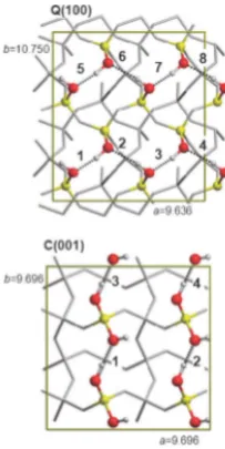
1.8 Schematic of the quartz(100)- and cristobalite(001) surfaces adapted

from Sodupe et. al.4 Red represents oxygen atoms, white hydrogen

(10)

1.9 Si-O hydrolysis for hydrated Ca2+, with outer sphere paths shown in

red, inner sphere paths shown in red as adapted and the barrier to

hy-drolysis in the absence of ions in black from Doveet. al.5 . . . 19

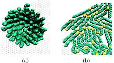
1.10 Flat physiosorbed ODT molecules on Au(111) (left) and chemisorbed ODT molecules on Au(111) (right) as adapted from Ahnet. al.6 . . . . 29

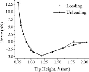
1.11 Interaction force on approach and retration of the wall to the gold sphere from Patricket. al.7 . . . 32

2.1 Schematic of the bond between atomsiandj. . . 37

2.2 Schematic of the angle made between the atomsi,jandk . . . 37

2.3 Schematic of a proper dihedral angle. . . 38

2.4 Schematic of a improper dihedral angle. . . 38

2.5 Exemplar Lennard-Jones Potential Energy Curve. . . 39

2.6 Schematic of periodic boundary conditions. . . 44

2.7 Schematics of a potential energy landscape (PEL): 3D (left) and 2D (right) representations. . . 45

2.8 Structure of the model amorphous silica surface used in the MD simula-tions: (a) side on view (b) view of the surface in thexy-plane (c) zoomed in side-on view (d) zoomed in view of the surface in thexy-plane. The different types of silanol are denoted UL, LL and R, as labelled. . . 53

2.9 Schematic to illustrate the concept of surface roughness and the slices used for binning the data. . . 59

(11)

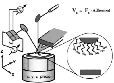
2.12 Schematic of the CFM-AFM setup, as adapted from Lieberet. al.9 The

sample is positioned on a piezoelectric xyz translator. A laser beam is

reflected from the tip onto a photodiode to detect the force experienced

by the tip. The movement of the tip up and down reflects the force

experienced by the tip. . . 64

2.13 Schematic of approach and retration curvesStippet. al.8. . . 65

3.1 Structures of the tripeptides (a) RGD (b) SPT. Backbone atoms are

highlighted in red andΦandΨdihedral angles marked. . . 70

3.2 2D representation of the bonds involved in a dihedral angle centred on

the black bond, with the corresponding Newman projections for a

se-lection of angles. . . 70

3.3 Ramachandran plots for the four cases (a) RGD with TIPS3P (b) RGD

with SPC/Fw (c) SPT with TIPS3P and (d) SPT with SPC/Fw. Note that

φ andψ are both periodic, and so some of the regions are split across

boundaries . . . 71

3.4 Population distribution over regions of the Ramachandram plots. (a)

RGD; regionsa-gare defined in Figure 3.3(a). (b) SPT; regionsa-bare

defined in Figure 3.3(c). . . 72

3.5 Pictorial diagrams of representative structures from regions (a) g and

(b)b. The backbone is shown in yellow and the central bonds ofΦand

Ψangles are labelled. For regiong, bond distances between key atoms

have been displayed. H-bonds are labelled by the bold, black lines. . . . 73

3.6 Distribution of transitions between regions of the Ramachandran plots

for RGD (a) TIPS3P (b) SPC/Fw. The labels of the x-axis indicate the

initial state and colour indicates the final state. Region h represented

the area of the plot not defined by boundaries. . . 75

3.7 Number of clusters as a function of simulation timestep (a) RGD,

back-bone; (b) RGD, peptide; (c) SPT, backbone (d) SPT, peptide . . . 77

3.8 Population distribution of RGD clusters over 50 ns. Inset: as the main

graph, but on a semi-log scale. (a) backbone and (b) peptide. Analogous

(12)

3.9 Population distribution of RGD for the top four clusters, for (a)

back-bone and (b) peptide clusters, using TIPS3P cluster IDs. Analogous

data for SPT are given for (c) backbone and (d) peptide clusters, using

TIPS3P cluster IDs. Standard errors are given to 95% confidence (a)

backbone (b) peptide. . . 79

3.10 Centroid (as defined in section 2.1.3) cluster structures for the top four

peptide clusters of RGD obtained using the TIPS3P model. . . 82

3.11 Exemplar RDFs for RGD: (a) gO−HW(r) between the oxygen atoms of

the terminal carboxylate group and the hydrogen atoms of water and (b)

gO−OW(r) between the oxygen atoms of the terminal carboxylate group

and the oxygen atoms of water. . . 87

3.12 Histograms of different aspects of the hydrogen bonds between the

pep-tide and water for (a) distances (b) angles. Distributions were the same

for both the RGD and SPT peptides. . . 88

3.13 The percentage growth of the different regions of the RGD

Ramachan-dran plot as a function of simulation timestep for the two water models

(a) TIPS3P (b) SPC/Fw. Regionhagain represented all the areas of the

plot that were not defined by boundaries. . . 89

3.14 Replica pathway of the initial ’replica 0’ for the RGD system as an

example for (a) TIPS3P (b) SPC/Fw. . . 90

3.15 The effect of the length of time between replica exchange attempts on

the growth of clusters in the RGD system as an example for (a)

back-bone (b) peptide. . . 91

4.1 Schematic to show the start structure (left), optimised structure (centre)

(13)

4.2 Ion concentration as a function of distance from the surface for the ions

in the NaCl, KCl, CaCl2and MgCl2solutions (low salinity - LS 0.1 M,

high salinity - HS 0.3 M). Cation concentration is represented by black

and anion concentration is represented by red. For these two colours,

the solid lines represent LS solution and the dashed lines HS. However,

in the majority of cases only the dark blue function is visible, as it

over-lays the light blue. LS and HS refer to the ’bulk’ concentrationsi.e.the

concentrations far from the surface. . . 98

4.3 Schematic of how the thickness of the EDL was calculated from ion

density distributions, using aqueous NaCl as an example. . . 99

4.4 Rdfs between the deprotonated silanol O− and all cation types studied

(Na+, K+, Ca2+ and Mg2+) and rdf between Ca2+₍_O−₎ions and Cl−. . . . 100

4.5 Contribution to the surface density profile arising from cations

asso-ciated with the first peak of the deprotonated silanol-cation rdfs

(Fig-ure 4.4), CSDP(O−-Mrdfp1) . Analogous data is given for the

sec-ond rdf peak for MgCl2(CSDP(O−-Mg2+rdfp2)) and the first rdf peak

of the O−-associated calcium-chloride rdf CSDP(O−Ca2+-Cl−rdfp1).

The complete surface density profiles are reproduced from Figure 4.2

to aid comparison. As in Figure 4.2, cation concentration is represented

by black and anion concentration is represented by red. Green

repre-sents the CSDP(O−-Mrdfp1) and, for MgCl2, pink is the CSDP(O−

-Mg2+rdfp2). Orange represents the CSDP(O−Ca2+-Cl−rdfp1). The

solid lines represent LS solution and the dashed lines HS. In part c)

of this diagram, the CSDP(O−-Ca2+rdfp1) overlays the complete Ca2+

density profile and CSDP(O−Ca2+-Cl−rdfp1) the Cl− density profile

for both LS and HS. . . 102

4.6 ρZmax(xy) (i.e. lateral distribution of cations found within a horizontal

layer of thickness 0.1 ˚Aand centred on the peaks in density as shown

in Figure 4.2c) for CaCl2solution (LS 0.1 M). The units of the number

density are arbitrary and the same in all lateral profiles throughout this

(14)

4.7 ρZmax(xy) (i.e.lateral distribution of Cl− ions found within a horizontal

layer of thickness 0.1 ˚A and centred on the peaks in density as shown

in Figure 4.2c) for CaCl2solution (LS 0.1 M)). The units of the number

density are arbitrary and the same in all lateral profiles throughtout this

section. . . 106

4.8 Schematic of the angle made between the surface normal and the O−

-M+ vector. . . 107

4.9 Distributions of the angle made between the surface normal and: (a)

rCa−O, where rCa−O = rCa - rO (b) rCl−O, where rCl−O = rCl - rO. p

refers to the particular peak in the CSDP(rdfp1) and n Cl−indicates the

distributions when n Cl− ions were associated. Cos(θ) distributions are

presented in Appendix C. . . 108

4.10 Distributions of the distances to the three different protonated silanols

for Ca2+ ions in peak 1 and 2 of thez-density distributions (LS, 0.1 M

and HS, 0.3 M). UL stands for upper left, LL lower left and R right and

are defined in Figure 2.8. . . 109

4.11 Distributions of the angle made between the surface normal and rCl−O,

where r_Cl₋_O = r_Cl - rO (CaCl2) (LS 0.1 M). p refers to the particular

peak in the CSDP(rdfp1) . . . 110

4.12 CSDP arising from Ca2+that have chloride ions from a particular peak

(p = p1, p2, ... where p1 is the first peak, etc) in the Cl− z-density

distribution associated with them The complete surface density profiles

for Ca2+ z-density are reproduced from Figure 4.2 to aid comparison.

As in Figure 4.2, cation concentration is represented by black and the

solid lines represnet LS solution, while the dashed lines represent HS.

The CSDP is given in solid lines of different colours in both the LS,

0.1 M subfigure (a) and the HS 0.3 M subfigure (b): Orange for Ca2+

with Cl− from p1 of the Cl− z-density profile, pink for p2, light green

(15)

4.13 ρZmax(xy): lateral cation density profiles at maxima in the ion

concen-trationvs distance from the surface distributions for KCl solution (LS

0.1 M). The units of the number density are arbitrary and the same in

all lateral profiles throughout this section. (Note that the graph for K+

peak 1 is zoomed-in compared to those of the other peaks, to show the

smaller areas of high density in a greater level of detail.) . . . 114

4.14 Schematic of the adsorption of Cl−to surface adsorbed Ca2+at an angle

of∼89◦with respect to the surface normal. . . 117

4.15 Water density as a function of distance from the surface for the NaCl,

KCl, CaCl2and MgCl2solutions (low salinity - LS 0.1 M, high salinity

- HS 0.3 M). The solid lines represent LS solution and the dashed lines

HS. . . 118

4.16 ρZmax(xy) for water density (within a horizontal layer of thickness 0.1 ˚Aand

centred on the peaks in density as shown in Figure 4.15) for 0.1 M NaCl

solution and 0.1 M MgCl2. OnlyρZ p3(xy) is shown here for the latter

solution, as those for the first two were not significantly different in

character to those of the other solutions. The labelsSAandSBare used

to highlight different structural characters. . . 120

4.17 Rdfs between O− and the hydrogen atoms of water for all electrolyte

solutions. . . 121

4.18 Rdfs between O− and the oxygen atoms of water for all electrolyte

solutions. . . 121

4.19 Surface topology: van der Waals representation of the amorphous silica

surface. . . 121

4.20 ρZmax(xy) for water density (within a horizontal layer of thickness 0.1 ˚Aand

centred on the peaks in density as shown in Figure 4.15) for CaCl2

solution at ionic strengths of 0.1 M and 0.3 M. The labels are used to

highlight different structural characters that correspond to different

(16)

4.21 Water Density and ion concentration as a function of distance from the

surface for the ions in the NaCl, KCl, CaCl2and MgCl2solutions (low

salinity - LS 0.1 M, high salinity - HS 0.3 M). Cation concentration is

represented by black and anion concentration is represented by red. For

these two colours, the solid lines represent LS solution and the dashed

lines HS. Light blue represents H2O from LS solution and dark blue

represents H2O from HS solution. However, in the majority of cases

only the dark blue function is visible, as it overlays the light blue. LS

and HS refer to the ’bulk’ concentrations i.e. the concentrations far

from the surface. Ion concentration distributions are reproduced from

Figure 4.2 and water density distributions are reproduced from Figure

4.15. O− density is shown as a pink line on the plots. A lateral density

profile of the water represented by the second peak in the water density

(at ∼3 ˚Afrom the surface) is shown in Figure 4.20 (CaCl2, 0.1 M and

0.3 M) and Figure 4.16 (NaCl, representative of all other solutions).

Lateral water density profiles for the KCl and MgCl2cases are given in

Appendix C, Figure C.9. . . 126

4.22 Net water orientation as a function of distance for a selection of the

electrolyte solutions investigated. The uncertainties are standard errors

given to 95 % confidence. Lateral water orientation profiles, with the

lateral location of SiO− and SiOH groups superimposed, are shown

in Figures 4.25 and 4.26 and show how waters partition between the

different functional groups of the surface. . . 129

4.23 P(cos(θ)) distributions were calculated between distances of 4-4.5 ˚A

(black), 4.5-5 ˚A (red), 5-5.5 ˚A (green) and 5.5-6 ˚A (pink). The solid

lines represented 0.3 M CaCl2solution and the dotted lines represented

0.1 M NaCl. . . 130

4.24 P(cos(θ)) distributions between 6.5-12.5 ˚A for (a) 0.3 M CaCl2denoted

(17)

4.25 Exemplar ori_Z₍₄_.₅₋₅₎(xy) (lateral water orientation) profiles. U1

rep-resents O−, U2, O−Ca2+, U3, O−Ca2+Cl− and U4, O−Ca2+Cl−2.

Blue dots represent the superimposed lateral locations of deprotonated

silanol oxygens (O−) and the green dots represent those of protonated

silanol oxygens. . . 133

4.26 Exemplar ori_Z₍₅_.₅₋₆₎(xy) (lateral water orientation) profiles. U1

rep-resents O−, U2, O−Ca2+, U3, O−Ca2+Cl− and U4, O−Ca2+Cl−2.

Blue dots represent the superimposed lateral locations of deprotonated

silanol oxygens (O−) and the green dots represent those of protonated

silanol oxygens. . . 134

4.27 Perpendiular (’perp.’) and Parallel (’lat.’) Diffusion as a Function of

Distance from the Surface for water and cations in 0.1 M NaCl solution. 137

5.1 AFM force mapping data: the average maximum adhesion during an

AFM approach-retract cycle (full method details in Section 2.2.2 of (a)

NH3+and (b) COOH/COO−functionalized tips during interaction with

the amorphous silica during exposure to the solutions at low salinity

(LS) 0.1 M and high salinity (HS) 0.3 M. The labels 1 and 2 in the Ex-periment ID are used to denote the exEx-periment number as salinity was

cycled twice between LS and HS concentrations. . . 145

5.2 A high resolution image in normal AFM mode of the surface scanned

in our study (amorphous silica). . . 145

5.3 Graphical representations of the different possible states for surface

de-protonated oxygens in CaCl2solution. Ca2+ions are represented by the

dark blue atoms and Cl− ions are represented by the green atoms. (a)

unoccupied O− (b) Ca2+ occupied O− (c) upright Ca2+Cl− occupied

O− (d) flat Ca2+Cl− occupied O− (e) Ca2+Cl−2occupied O−. . . 147

5.4 Initial free energy profiles from metadynamics simulations (a) NaCl

-after 180 ns (b) KCl - -after 130 ns (c) CaCl2- after 130 ns (d) MgCl2

(18)

5.5 NaCl LS - several demonstrations that the metadynamics simulations

had not converged (a) Evolution of the free energy profile with time.

(b) Free energy difference between 2 distinct points of the free energy

profile with time. Comparison to high salinity included. (c) Histogram

of CV space explored over the final 25 ns. Comparison to high salinity

included. . . 150

5.6 NaCl LS, a smaller volume of CV space - several demonstrations that

the metadynamics simulations had not converged (a) Evolution of the free energy profile with time (b) Free energy difference between 2

dis-tinct points, the minimum centered at ∼ 0.25 nm and a point in the

plateau region, of the free energy profile with time (c) Histogram of CV

space explored over the final 20 ns. . . 152

5.7 Lateral free energy profiles taken over the total volume of available CV

space for the entire metadynamics simulations (a) low salinity NaCl,

80 ns (b) low salinity CaCl2, 27 ns. . . 153

5.8 Evidence of convergence (a) Distribution of CV (distance from surface)

values (b) Evolution of the free energy profile with time (c) Free energy difference between points marked ’FED1’ on Fig 5.8b as a function

of time (d) Free energy difference between points marked ’FED2’ on

Fig5.8b as a function of time . . . 155

5.9 Two examples of the free energy profiles from the final

metadynam-ics simulations, a comparison between the corrected and uncorrected

versions for (a) low salinity aqueous NaCl and (b) the O−Ca2+Cl−2

adsorption site configuration, low salinity aqueous CaCl2. . . 157

5.10 Free energy profiles determined from the MD simulations for the

ad-sorption of N to the silica surface in (a) NaCl solution (b) MgCl2

solu-tion, Mg2+-occupied O−. . . 158

5.11 Lateral free energy profiles at distances from the surface for the major

minima (at 3.2, 3.5 and 3.9 ˚A from the surface) in the low salinity NaCl

solution. The lateral positions of the surface oxygen are superimposed

(19)

5.12 Lateral free energy profiles at distances from the surface for the

ma-jor minima (at 3.2, 3.6 and 4.0 ˚A from the surface) in the low salinity

MgCl2solution. The lateral positions of the surface oxygen are

super-imposed on the free energy profile. . . 161

5.13 Free energy profiles determined from the MD simulations for the

ad-sorption of N to the silica surface at different O−-based adsorption site

configurations in CaCl2solution (a) unoccupied O− (b) Ca2+occupied

O− (c) flat Ca2+Cl− occupied O− (d) Ca2+Cl−2occupied O− . . . 162

5.14 Lateral free energy profiles at distances from the surface for the major

minima (as defined in the main text) in aqueous LS CaCl2at unoccupied

O−. The lateral positions of the surface oxygen are superimposed onto

the free energy profile. . . 164

5.15 Lateral free energy profiles in aqueous low salinity CaCl2 for various

attachments at O− at the distance of (a) minimum 1 (2.1-2.45 ˚A), (b)

minimum 2 (3.7 ˚A). The lateral positions of the surface oxygen are

su-perimposed onto the free energy profile. . . 165

5.16 Lateral free energy profiles at distances from the surface for minimum

2 (2.1-2.45 ˚A) in aqueous low salinty CaCl2 for various attachments at

O−. The lateral positions of the attached Ca2+ are represented as red

crosses superimposed onto the free energy profile and appeared as a

single continuous region that is slightly elongated away from the

am-monium adsorption site. . . 167

5.17 (a) Lateral free energy profile for the CaCl2attachment at O−at the

dis-tance of minimum 2 (3.7 ˚A). The lateral positions of the surface oxygen

are superimposed onto the free energy profile. The positions of

particu-lar bridging oxygens have been labelled ’1’, ’2’ and ’3’. (b) Schematic of corresponding physical system with the same bridging oxygens

la-belled ’1’, ’2’ and ’3’. Apart from the lala-belled ions, Ca2+ and Cl−,

oxygen atoms are shown in red, silicon in yellow, hydrogen in white,

(20)

5.18 The force curves were generated by taking the gradient of the free

en-ergy profiles for methylammonium adsorption in solutions of NaCl and

CaCl2specifically where Ca2+Cl−2is associated with the deprotonated

surface oxygen. . . 169

5.19 Replica mobility in the MD simulation using the more efficient REST

technique10 for 72 replicas. . . 170

6.1 Schematic of the starting configuration of the model tip simulation at a

certain distance from the surface. The gold atoms of the tip are shown

in pink, with attached orgnics (bright blue C, dark blue N and white H),

Cl− ions are green and Ca2+ ions dark blue, silcon atoms are yellow,

oxygen atoms are red and hydrogen white. . . 175

6.2 (a) Force experienced by the model tip atoms and (b) average minimum

N atom distance to the silica surface when the gold and sulfur atoms

of the model tip were restrained at different distances from the surface.

For (b), ’min 1’ and ’min 2’ mark the approximate position of minimum

1 and the exact position of minimum 2 for the different adsorption site

configurations in at the aqueous CaCl2/silica interface. . . 177

B.1 RDFs gO−HW(r) between RGD’s (a) oxygen atoms of the sidechain

car-boxylate group (b) nitrogen atoms of the guanidinium group (c)

ammo-nium nitrogen atom and the hydrogen atoms of water. RDFs gO−OW(r)

between RGD’s (d) oxygen atoms of the sidechain carboxylate group

(e) nitrogen atoms of the guanidinium group (f) ammonium nitrogen

atom and the oxygen atoms of water . . . 214

B.2 Exemplar RDFs for RGD: (a) gO−HW(r) between the oxygen atoms of

the terminal carboxylate group and the hydrogen atoms of water and (b)

gO−OW(r) between the oxygen atoms of the terminal carboxylate group

and the oxygen atoms of water. . . 215

B.3 Dihedral angle distributions for (a) terminal N-Cα-Cβ-Cγ, residue R (b)

Cα-Cβ-Cγ-Cδ, residue R (c) Cβ-Cγ-Cδ-sidechain N, residue R (d) Cγ

-C_δ-sidechain N-C_δ-Cε, residue R (e) N-Cα-Cβ-Cγ, residue D (f) Cα

(21)

B.4 The percentage growth of clusters for the RGD peptide as a function

of simulation timestep for (a) TIPS3P, backbone (b) SPC/Fw, backbone

(c) TIPS3P, peptide (d) SPC/Fw, peptide. . . 217

B.5 Replica pathway of the initial ’replica 0’ for the SPT system for (a)

TIPS3P (b) SPC/Fw. . . 217

C.1 ρZmax(xy): lateral cation density profiles at maxima in the ion

concen-tration vsdistance from the surface distributions for NaCl and MgCl2

solutions (LS 0.1 M). The units of the number density are arbitrary and

the same in all lateral profiles throughout this section. . . 220

C.2 ρZmax(xy): lateral cation density profiles at maxima in the ion

concen-trationvsdistance from the surface distributions for NaCl, KCl, CaCl2

and MgCl2 solutions (HS 0.3 M). The units of the number density are

arbitrary and the same in all lateral profiles throughout this section. . . . 221

C.3 ρZmax(xy): lateral Cl− density profiles at maxima in the ion

concentra-tion vs distance from the surface distributions for CaCl2 solution (LS

0.3 M). The units of the number density are arbitrary and the same in

all lateral profiles throughout this section. . . 222

C.4 Distributions of the angle made between the surface normal and rM−O,

where rM−O= rM - rO. p refers to the peak in the CSDP(O−-Mrdfp1). . 223

C.5 Distributions of the angle made between the surface normal and rM−O,

where rM−O= rM - rO. p refers to the peak in the CSDP(O−-Mrdfp1). . 224

C.6 Distributions of cos(θ) whereθ is the angle made between the surface

normal and: (a) rCa−O, where rCa−O= rCa - rO (b) rCl−O, where rCl−O

= rCl - rO. p refers to the particular peak in the CSDP(rdfp1) and n Cl−

indicates the distributions when n Cl− ions were associated . . . 225

normal and rM−O, where rM−O = rM - rO. p refers to the peak in the

CSDP(O−-Mrdfp1). . . 226

normal and rM−O, where rM−O = rM - rO. p refers to the peak in the

(22)

C.9 ρZmax(xy): additional lateral water density profiles at maxima in the

water density vs distance from the surface distributions for KCl and

MgCl2 solution (0.1 M). Blue dots represent deprotonated silanols and

green dots reprent protonated silanols. The units of the number density

are arbitrary and the same in all lateral profiles throughout this section. . 228

C.10 ρZmax(xy): lateral water density profiles at maxima in the water density

vs distance from the surface distributions for NaCl, MgCl2and CaCl2

solution (0.3 M). The units of the number density are arbitrary and the same in all lateral profiles throughout this section. . . 229

C.11 ρZmax(xy): Lateral water density profiles at maxima of the secondary

layers in the water densityvsdistance from the surface distributions for

0.3 M CaCl2solution and at the counterpart distances in 0.1 M solution.

The units of the number density are arbitrary and the same in all lateral

profiles throughout this section. . . 230

C.12 Net water orientation as a function of distance for a selection of the

electrolyte solutions investigated. . . 231

C.13 Full distributions of cos(θ) between 0-2.5 ˚A and between 2.5-4 ˚A for

0.3 M CaCl2denoted Ca and 0.1 M NaCl, denoted Na. . . 232

C.14 Full distributions of cos(θ) between 4-6 ˚A for 0.1 M and 0.3 M CaCl2. . 232

D.1 RDFs between (a) O−to ’bound’ Ca2+(b) Ca2+to ’bound’ Cl−(c) O−

to ’bound’ Cl− . . . 234

D.2 rdfs between (a) O− bound Ca2+ and all chloride ions apart from any

officially associated Cl−. (b) O−and all Ca2+ions. . . 235

D.3 Cation-deprotonated oxygen and chloride ion-surface bound calcium

(23)

D.4 The remainder of the free energy profiles from the final

metadynam-ics simulations, a comparison between the corrected and uncorrected

versions for (a) HS aq. NaCl (b) LS aq. KCl (c) HS aq. KCl (d)

un-bound state, LS aq. MgCl2(e) unbound state, HS aq. MgCl2(f) bound

state, LS aq. MgCl2 (g) O−, aq. LS CaCl2 (h) O−, aq. HS CaCl2 (i)

O−Ca2+, aq. LS CaCl2 (j) O−Ca2+, aq. HS CaCl2 (k) O−Ca2+Cl−,

aq. LS CaCl2(l) O−Ca2+Cl−, aq. HS CaCl2(m) O−Ca2+Cl−2, aq. LS

CaCl2(n) O−Ca2+Cl−2, aq. HS CaCl2 . . . 236

D.5 Free energy profiles for the adsorption of the nitrogen of

methylammo-nium to the silica surface in different salt solutions (a) KCl (b) MgCl2

solution, unoccupied O− . . . 237

E.1 Evidence for the equilibration of the inifinitely-sized monolayer. SP

refers to starting point. (a) water density as a function of distance from

the vacuum/gold surface (b) Cl− density as a function of distance from

the vacuum/gold surface (c) N density profiles as a function of distance

from the vacuum/gold surface (d) monolayer thickness with time (e) tilt

angle with time (f) azimuthal tilt angle with time. . . 239

E.2 Evidence for the equilibration of the system that featured the model

AFM tip and the model tip as a reasonable representation of the

in-ifinite monolayer (a) water density as a function of distance from the

silica surface (b) Cl− density as a function of distance from the

sil-ica surface (c) Ca2+ density as a function of distance from the silica

surface (d) maximum N atom distance from the surface - minimum N

atom distance from the surface (e) tilt angle of each of the Au-adsorbed

molecules with time (f) mean square displacement of the N atom of the

(24)

(25)

Acknowledgments

First and foremost I would like to acknowledge my two supervisors Tiffany Walsh and Mark Rodger, a synergistic team! I have enjoyed working with them and learnt alot from both: Mark my supervisor here at Warwick and Tiff in my first year here and throughout, a strong presence even from the other side of the world! I will miss this chapter in my life.

I thank Susan Stipp for the opportunity to visit her labs at The University of Copen-hagen, as well as Tue Hassenkam and Klaus Juhl for sharing their expertise and train-ing me in force-mapptrain-ing AFM. The entire NanoGeoScience Group made me feel very welcome and I would like to extend particular thanks for this to B¨arbel Lorenz, Akin Budi, Johanna Generosi and Dominique Tobler.

Special thanks to Louise Wright for advice, wisdom and friendship throughout, Aaron Finney for constructive criticism of this thesis and encouragement in general, particu-larly in the final stages of this PhD and my graphics guru, Annalaura Del Regno. Thanks to my office mates (current and past) and those based in the CSC: Julia Choe, Alaina Emmanuel, Chimie Gamot, Salvatore Cosseddu, Chinedu Nwaigwe, Yuanwei Xu, Paul Oluwunmi, Yuriy Bushuev, Tony Zhang, Minsouk Kim, Iresha Atthanayake, Toon Vasit Sirilapanan, David O’Neill, Jenny Webb, David Bray, Aaron Brown and Oliver Yang.

Thanks to the wider scientific community at Warwick and beyond: Gil Rutter, Marina Cendic, Stepan Ruzicka, Matt Bano, Bart Vorselaars, Max Saller, Boy Lankhaar, Lewis Baker, Anja Humpert, Rebecca Notman, Scott Habershon, David Quigley, Mike Allen, my advisory board Ale Troisi and Rob Deeth, those of the mIb consortium and many more, including those I haven’t mentioned but nonetheless have meant alot along the journey!

Thanks to the CSC computing and adminstrative staff: Vida Glanville, Christine Jarvis, Natalie Tyldesley Marshall, Magnus Lewis-Smith, Grok (Jaroslaw Zachwieja), Olav Smorholm, Marius Bakke and Matthew Ismail.

(26)

Declarations

This thesis is my own work. Results based on collaborative efforts have been explicitly

stated in the text (Chapter 5). No part of this report has been previously submitted for

examination for any other higher degree or for a degree at an establishment other than

the University of Warwick. The work of Chapter 3 has been published as the following

journal article: J. L. Desmond, P. M. Rodger and T. R. Walsh, Mol. Sim., 2013, 40,

(27)

Abstract

Low-salinity enhanced oil recovery (EOR) uses low-salinity seawater in the water flooding of sandstone reservoirs to maximise oil yields. Because oil is strongly ad-sorbed onto mineral surfaces, understanding the interactions involved at the oil/mineral interface, and how to weaken them, is crucial to design more efficient, low-cost EOR.

This thesis focuses on the influence of electrolyte concentration on the

interac-tion of alkylammonium (R-NH+₃) and alkylcarboxylic acid/carboxylate (R-COOH/COO−

functionalities, present in crude-oil, with the amorphous silica (mimic for quartz grains in sandstone)/aqueous electrolyte interface. Both computational (molecular dynamics, MD) and experimental (chemical force mapping atomic force microscopy, CFM-AFM) techniques were used.

Firstly (Chapter 3), we tested the inter-operability of the new SPC/Fw water force-field with CHARMM. No significant differences were found between the data generated from SPC/Fw-CHARMM and TIPS3P-CHARMM, therefore the latter, com-putationally more efficient, was used in Chapters 4-6.

The behaviour of the four electrolyte solutions at two concentrations was tested

in Chapters 4-5 (NaCl, KCl, CaCl2 and MgCl2 at 0.1 and 0.3 M); interfacial ion and

water structuring has been investigated in Chapter 4, while the effect of the electrolytes

on the adsorption of R-NH+₃) and alkylcarboxylic acid/carboxylate (R-COOH/COO−

was explored in Chapter 5. Interfacial ion concentration was greatest in the CaCl2case,

with various long-lived surface-site types involving different combinations of ions iden-tified. CFM-AFM showed a substantial concentration-dependent difference in adhesion

for R-NH+₃ in CaCl2and R-COOH/COO− in the divalent ion solutions.

The free energy of adsorption for NH+₃CH3was investigated using

metadynam-ics. Force curves were calculated from the generated free energy profiles. The greatest

force is, indeed, observed for one particular surface-site type in CaCl2 solution,

preva-lent in more concentrated solutions.

Finally, a more sophisticated computational model for the experimental AFM

tip, a small array of S(CH211NH3+, is presented in Chapter 6, laying the basis for

(28)

Abbreviations

ADF Angular Distribution Function

AFM Atomic Force Microscopy

AIMD Ab InitioMolecular Dynamics

ASW Artificial Seawater

CFM-AFM Chemical Force-Mapping Atomic Force Microscopy

COM Centre of Mass

CSDP Contribution to the Surfacez-density Profile

CSDP(O−-MrdfpN Contribution to the Surfacez-density Profile for ions in the Nth peak in the silica

surface O− to cation rdf

CV Collective Variable

DFT-MD Density Functional Theory-Based Molecular Dynamics

EDL Electrical Double Layer

EOR Enhanced Oil Recovery

Ex. P. Exchange Probabilities

(29)

FEP Free Energy Perturbation

FES Free Energy Surface

GCS Gouy-Chapman-Stern

HCP Hexagonal Close Packed

H-REMD Hamiltonian Replica-Exchange Molecular Dynamics

HS High Salinity (0.3 M)

H-S Helmholtz-Smoluchowski

IDP Intrinsically Disordered Protein

IEP Isoelectric Point

LJ Lennard Jones

LLO Lower Left Oxygen

LS Low Salinity (0.1 M)

MD Molecular Dynamics

metaD Metadynamics

MSD Mean Squared Displacement

N the NH3+Group of Methylammonium

NEMD Non-Equilibrium Molecular Dynamics

No. Ex. Number of Exchanges

(30)

NMR Nuclear Magnetic Resonance

NVT Canonical Ensemble (constant number, volume and temperature)

ODT 1-Octadecanethiol

ori_Z₍_z₁₋_z₂₎(xy) lateral water orientation profiles, where z1 is the z-distance from the surface

where the horizontal slice starts and z2 is where it ends.

p1 Peak 1

p2 Peak 2

P(cos(θ)) Full cos(θ) distributions

P2VP poly(2-vinylpyridine]

PEL Potential Energy Landscape

PME Particle Mesh Ewald

PMF Potential of Mean Force

PZC Point of Zero Charge

rdf Radial Distribution Function

REMD Replica-Exchange Molecular Dynamics

RMSD Root-Mean Squared Deviation

REST Replica-Exchange with Solute Tempering

RO Right Oxygen

(31)

SFG Sum-Frequency Generation

SHG Second Harmonic Generation

T-REMD Temperature Replica-Exchange Molecular Dynamics

ULO Upper Left Oxygen

vdW van der Waals

WT Well-Tempered

XPS X-ray Photoelectron Spectroscopy

XR X-ray Reflectivity

ZPC Zero Point Charge

ρZmax(xy) lateral density profile for ions within a small range ofz-distances from the surface

centered at the Nth peak in ionz-density. Zmax is equal to ZpN (the Nth peak in

(32)

Chapter 1 Introduction

1.1 Aim: Understanding the ’Low Salinity’ (LS) Effect

and Enhanced Oil Recovery (EOR)

The influence of ionic strength on the molecular adsorption of polar compounds is of

particular importance to the investigation of enhanced oil recovery, EOR (a collection

of techniques used to increase yields of crude oil from oil reservoirs, one of which is

low-salinity EOR). Indeed, the main aim of this thesis was to increase understanding

of the ’low salinity’ effect (as defined in section 1.1.1) and thus low salinity EOR, with a particular focus on low salinity EOR from sandstone reservoirs. Since current oil

recovery methods may leave up to 65 % of the original oil in the reservoir, the need

for improved understanding of low-salinity EOR is clear.11 Amorphous silica was

con-sidered as a model for sandstone, the R-NH+₃ and R-COOH/COO− functional groups

were selected as mimics for the polar components of oil and the aqueous electrolytes

represented the different ionic components present in seawater. The mineral

composi-tion of sandstone is dominated by silica, as quartz and it is assumed that oil is exposed

to this material in the pores of sandstone reservoirs.8 Amorphous silica (Figure 1.1) and

natively-oxidised silicon (Figure 2.8) surfaces are often used as models for exploring

the behavior of the surfaces of quartz grains in sandstone.8 The polar functionalities,

R-NH+₃ and R-COOH/COO−, were selected for investigation, as the presence of polar

functionalities in crude oil is a requirement for the ’low salinity’ effect to be observed.8

(33)

aliphatic amines, is small, the interaction of the functionality with the aqueous

elec-trolyte/amorphous silica interface is thus far underexplored.12, 13 The use of chemical

force mapping atomic force microscopy, CFM-AFM (described in Chapter 2, section

2.2.1) and molecular simulation (described in Chapter 2) is an excellent way to study

in-terfacial phenomena, with the CFM-AFM providing macroscopic adhesion force values

and the simulation giving atomistic-level insight. In this thesis, a combined

experimen-tal/simulation approach has been taken, using both techniques. In experiment, an AFM

tip has been functionalised with long-chain hydrocarbons terminated by the desired

functionality (both NH+₃ and COOH/COO− have been analysed in this way). In

simu-lation, the focus has been on the interaction of the R-NH+₃ functionality at the aqueous

electrolyte/amorphous silica interface. This was explored initially with a single

methy-lammonium molecule and then, in a more complex model of the experimental AFM

tip, as an array of long-chain hydrocarbons terminated with NH+₃. The introduction has

been structured by first discussing the main motivation for this work and how it will be

explored, wider-ranging applications of the silica/aqueous electrolyte interface and then

experimental studies at the silica/water interface, the Gouy-Chapman-Stern model (a

commonly used theoretical model for charged surface/aqueous electrolyte interfaces), simulation studies at the silica/water interface, a mixed experimetnal/simulation

sec-tion concerning molecular adsorpsec-tion at the silica/water interface, including force-field

inter-operability, an important aspect of such simulations and atomic force microscopy

[image:33.595.257.376.485.602.2]

(AFM) by simulation, concluding with a detailed aims and objectives section.

Figure 1.1: Schematic of the amorphous silica/water interface adapted from Butenuth

(34)

1.1.1 The ’Low Salinity’ (LS) Effect

In EOR, there is clear evidence that production from sandstone reservoirs increases

when the water used to sweep the reservoir and to maintain pressure has salinity

be-low about 5000 ppm, compared to undiluted seawater of salinity 30000 ppm or more.14

Several hypotheses have been proposed to explain the mechanisms responsible for this

’low salinity’ (LS) effect, as described in a recent review by Sheng.15 A selection have

been discussed in detail.

Electric Double Layer (EDL) Expansion and Fines Migration Theory

The EDL is a description of the electric field at a charged interface, such as a charged colloidal particle or a flat surface in contact with water. It has been described in more

depth in section 1.4, where it is illustrated schematically in Figure 1.6. The depth of the

EDL can be predicted by DLVO theory, as described by Overbeeket. al.16 Further,

ac-cording to DLVO theory, the width of the EDL will increase as salinity decreases. In the

case of a negatively charged surface, negatively charged molecules in the interfacial

re-gion will become less strongly attracted to the surface as the width of the EDL increases

and the shielding of the surfaces negative charge by interfacial cations decreases. EDL

expansion is also key to fines migration theory.14 The greater the width of the EDL, the

more likely the interaction of colloidal EDLs and bulk clay swelling. In this theory, it

was proposed that the fine clay particles that result from such a process are released, along with associated oil.

Multicomponent Ionic Exchange

Various mechanisms have been proposed for the binding of oil to the sandstone surface.

Four mechanisms, believed to be important to the ’low salinity’ effect, are depicted in

Figure 1.2, with several examples of the functional groups likely to be involved in each

case.17 Ligand bridging (Figure 1.2a) and cation bridging (Figure 1.2b) both describe

mechansims where a multivalent cation forms bonds with a negatively charged oxygen

of the surface and a negatively charged organic molecule. The type of bonding,

how-ever, differs. In the ligand bridgng mechansim, it is covalent, whereas in the cation

briding mechanism it is ionic. For strongly solvated ions, for example Mg2+, a water

(35)

interacts with the organic molecule through dipole-dipole interactions (where the

posi-tive end of a polar molecule interacts with the negaposi-tive end of another polar molecule).

The cation exchange mechanism describes the process whereby interfacial cations are

replaced by positively charged organic molecules (Figure 1.2d). It is suggested that

monovalent ions readily replace divalent ions in ’low salinity’ water leading to the

dis-placement of organic molecules bound through the mechanisms shown in Figure 1.2a-c.

It has also been suggested to be an equilibrium effect, with the divalent ions that linked

organic molecules to the surface and were originally present in the higher salinity solu-tion moving away from the surface to reach equilibrium with the newly introduced low

salinity solution.18

Interfacial pH Effects

It has been proposed that the interaction of cations with the silica surface leads to the

formation of hydroxyl ions. The hydroxyl ions can deprotonate carboxylic acids present

in oil. If the carboxylic acid had been hydrogen-bonded (an attractive interaction

be-tween a highly electronegative atom,i.e. oxygen, nitrogen or fluorine, and a hydrogen

that is bonded to another highly electronegative atom) to the surface, this deprotonation

event will remove the hydrogen bonding mechanism and the acid may detatch from the

surface. This is shown by chemical equations in Figure 1.3.

Salt-In Effect

The solubility of organic compounds is affected by electrolyte concentration. Salting-in

describes the increase in solubility of organic compounds that occurs when the

elec-trolyte concentration is decreased. It is suggested that this may aid desorption from the

(36)

[image:36.595.177.455.112.501.2]

Figure 1.2: Schematic of the key briding mechanisms important to the ’low salinity’ effect and the functional groups through which they can occur.

(37)

1.1.2 ’Low-Salinity’ Enhanced Oil Recovery Mechanisms Explored

in This Thesis

Changes to the width of the EDL with concentration and electrolyte type and their

impact on molecular adsorption, have been explicitly explored in this thesis through the analysis of ion distributions in molecular dynamics (MD) simulations and calculation

of free energy of adsorption values using an advanced MD technique, metadynamics

(as will be described in Chapter 2, section 2.1.1). Concentration-dependent differences

give some insight to the fines migration theory hypothesis. However, since only a single

stationary silica surface was probed rather than a collection of mobile colloidal particles,

interaction of EDLs cannot be observed and a full testing of the hypothesis is beyond

the scope of this thesis. Furthermore, electrolyte-dependent differences in the EDL

reflect the various affinities of the ions for the silica surface, allowing testing of the

multicomponent ion exchange mechanisms.

1.2 The Aqueous Electrolyte/Mineral Interface

Aqueous electrolyte/mineral interfaces are ubiquitous in nature and technology, and

play a role in many commercial applications, such as solar cells, electronics and

biodegrad-able coatings of drug molecules.20 However, despite this and even though the ability

of minerals to induce dramatic structural changes to interfacial water has been

long-established,21 the physical details of such structure remain underexplored. This

interfa-cial solvent structure is important to understanding chemical processes occurring at the surface, such as mineral dissolution and molecular adsorption, processes which often

underpin the commercial applications.22, 23, 24

1.2.1 Importance of Biomolecule-Silica Interactions

Silica will be considered as a prototypical example. The mineral is terrestrially

predom-inant, featuring in various natural phenemona and applications, many of which involve

molecular adsorption at the interface of silica with physiological solution or seawater.20

The interaction of biomolecules with bioglass, a material primarily composed of silica,

(38)

body.25, 26 The adsorption behavior of polar compounds at the silica/aqueous electrolyte

interface is relevant to the understanding of enhanced oil recovery (EOR) from

sand-stone reservoirs.8 In nature, intrinsically disordered proteins (IDPs) - proteins which

lack a fixed three dimensional structure - and long-chain polyamines are involved in the

biomineralization of several silica-based structures, including the cell wall of marine

diatoms and skeletal form of Radiolarians.27, 28

1.2.2 A Brief Overview of Silica Literature to Date

Silica has been intensely studied as a substrate, and a wealth of experimental data is

available, as reviewed recently by Rimolaet. al.20 The properties and behavior of any

surface are controlled by its process history and silica is no exception.29, 20 For example,

if an amorphous silica sample is heated to more than 1000 K, condensation of surface

silanol groups irreversibly changes the surface structure, even after cooling and water

adsorption.30 The dependence of silica surface charge density on pH, cation type and

ionic strength of solutions has been extensively documented using various experimental

techniques, ranging from acid-base titration to evanescent cavity wave ring-down

spec-troscopy.31, 32, 33, 34, 35 Much of the past research efforts have been devoted to

investigat-ing the effect of ionic strength and electrolyte type on silica dissolution.36, 37, 38, 39, 40 Ion

specific adsorption is also an important aspect of the aqueous electrolyte/silica interface

interaction and has been widely studied.41, 42, 43, 44, 45

1.3 Experimental Studies at the Silica/Water Interface

Rimolaet. al. have noted two particularly enlightening studies concerning water

struc-ture at the interface between silica and water.20 The studies, both conducted in 2004,

reported regions of ’ice-like’ and ’liquid-like’ water. Shen and co-workers performed

sum frequency generation (SFG) spectroscopy experiments at the (0001) quartz/water

interface.2 The spectra featured two peaks, occuring at∼3200 cm−1, a position

nor-mally associated with the ice phase of bulk water, and ∼3400 cm−1 a position

cor-related with the less ordered, liquid water phase. The peak within the ’ice region’

became more intense with higher pH. At high pH, it is suggested that the increased

(39)

and deprotonated silanols. A different bonding mechanism, where silanols act as

hy-drogen bond donors to water, was proposed responsible at low pH. The two bonding

mechanisms have been illustrated in Figure 1.4. The suggestion was supported by SFG

phase measurements, which indicated that the dipole moment of the water molecules

was orientated oppositely at low and high pH. Engemannet. al. studied the amorphous

silica/ice interface using high-energy x-ray transmission reflection and found evidence

for a ’liquid-like’ interfacial ice layer.46 Further evidence for a difference in interfacial

solvent structure compared to that in bulk solution has been provided by various ex-perimental techniques, including nuclear magnetic resonance (NMR) spectroscopy and

neutron reflectivity with quartz crystal microbalance measurements.47, 48 These

stud-ies clearly demonstrate that solvent structure can be significantly modified by the silica

surface. No information, however, was given regarding the distribution of the ’ice-like’

and ’liquid-like’ regions.

Figure 1.4: Suggested predominant water interactions at the quartz/water interface at

low and high pH according to.2 The geometric criteria for defining a H-bond is

gen-erally when the distance between a heavy atom (O or N) and water oxygen is 3.5 ˚A or

less and when the angle between the acceptor and the donor hydrogen is 30◦or less.

With the aim of determining the distribution of ’ice-like’ and ’liquid-like’ water

at the fused-silica/aqueous electrolyte interface, Horeet. al. manipulated the width of

the interfacial region, the region responsible for the SFG signal, by varying the

con-centration of NaCl from 0 to 0.12 M.49 This exploited the well-accepted prediction of

DVLO theory that the higher the ionic strength, the smaller the width of the

(40)

decreased relative to that at ∼3400 cm−1 with increasing ionic strength (as the width

of the double layer decreased), it was concluded that the ice-like region existed further

from the surface. In otherwords, the data was interpreted to suggest that the character of

the water depended on proximity to the surface. This is in contrast to an interpretation

of SFG data at the quartz/water interface of Shen and co-workers that silanol groups of

different acidities were responsible for the two characteristic regions.50, 32 It is proposed

that in the ’ice-like’ regions, water molecules were more likely to bind to SiOH groups

viatheir oxygen atoms, compared to through their hydrogen atoms to SiO− groups in

’liquid-like’ regions.

1.3.1 The Effect of Ionic Strength

Rather than viewing ionic strength as a tool to change the Debye length (in otherwords,

the thickness of the electric double layer (EDL), a term which will be defined in section

1.4 and shown schematically in Figure 1.6), several experimental studies have explored

how ionic strength affects solvent structure at the aqueous electrolyte-silica interface.

Surface charge is particularly important, as demonstrated by Borguetet. al. in a study

concerned with the pH dependence of the addition of 0.1 M NaCl on SFG spectra taken

at the fused silica-water interface.51 The addition of salt only affected interfacial water

structure at pH values above the isoelectric point (IEP) of silica, when the surface was

negatively charged and ions were attracted into the interfacial region. At such pHs, the

addition of electrolyte ions resulted in a decrease in spectral intensity. The magnitude

of the influence of the electrolyte depended on pH and was greatest at near-neutral pH.

In a constant-pH study, Hore and co-workers varied the ionic strength of NaCl

solu-tion over a range from 0.05 mM to 4 M at a charged fused silica surface.52, 53 The peak

corresponding to ice-like water dominated until 1.1 M, when the peak associated with

liquid-like water became more predominant, with, it was suggested, ion adsorption dis-placing surface bound water molecules and disrupting the hydrogen bonding network.

It was suggested that in the low ionic strength regime there was a balance between the

decrease in intensity of the SFG signal,i.e. polar water ordering, as a consequence of

the decrease in interfacial depth and the increase in intensity due to the increased surface

charge. The latter factor dominated until∼0.7 M, when the signal began to decrease, in

(41)

played an important role in influencing interfacial water structure. This could be by

changing water orientation through altering surface charge or, at high ionic strength, by

adsorption of ions at the surface and disruption of the hydrogen bond network.

1.3.2 The Effect of Ion Type

The effect of ion type on the perturbation of interfacial water structure has also been

in-vestigated. Chou and co-workers recorded IR-visible sum frequency vibrational spectra at the interface of fused silica and a range of alkali chloride (LiCl, NaCl and KCl) and

sodium halide (NaCl, NaBr and NaI) solutions.54 In every case and as in previous

stud-ies, ’ice-like’ and ’liquid-like’ peaks appeared at their characteristic wavenumbers and

spectral intensity decreased with increasing ionic strength. Although alteration of the

anion had no significant impact on the spectral intensity, the degree of water

pertur-bation occurred in the order K+ >Li+ > Na+ for the alkali chloride solutions. The

authors proposed two factors to rationalize this behavior: the equilibrium constant of

hydrated cation association with SiO− groups (KK+>KNa+>KLi+) and the effective

ionic radii of the hydrated cations (rLi+ >rNa+ >rK+). A larger equilibrium constant

corresponds to a larger proportion of hydrated cation-associated siloxide groups and thus a greater perturbation of water structure. The larger the hydrated ion, the greater

the amount of water that would be displaced on its surface adsorption. Furthermore, the

peak associated with ’ice-like’ water was more vulnerable to cation perturbation than

the ’liquid-like’ peak. It was suggested that vicinal silanol groups (a schematic of the

different silanol types is shown in Figure 1.5) were responsible for the more ordered

ice-like structure and, with their higher local surface charge density compared to other

silanol types, were more likely to attract cations. In a vibrational sum frequency

spec-troscopy study at the negatively charged quartz-water interface, Cremeret. al. found a

correlation between the charge density of the cation and the extent of interfacial water

perturbation55 It was argued that the higher the charge density, the more favorable the

adsorption of the cation and the greater the disruption to interfacial water. The highly

charged Li+, however, was an anomaly to the trend. This was ascribed to Li+’s strongly

bound hydration shell and the concomitant decrease in it’s effective charge density. In

a parallel, anion-focused study at the same interface, Cremer and co-workers found the

(42)

and perturbation of water.56 Since the degree of surface ionization has been shown to

influence water perturbation, the effect of the electrolyte type on SiOH and SiO−

sta-bilization is also important. Using second harmonic generation (SHG) spectroscopy

at the aqueous fused-silica interface, Gibbs-Davis et. al. determined that for a range

of alkali chlorides, LiCl, KCl, CsCl and NaCl, only NaCl stabilized the deprotanated

state.57 Electrolyte identity did impact the degree of perturbation of interfacial water

structure and, as noted in one study, particularly disrupted regions of ’ice-like’ water.

A variety of ion-dependent characteristics were used to explain trends in the degree of interfacial water perturbation.

Figure 1.5: Schematic of the different silanol types: isolated, vicinal and geminal.

1.4 The Gouy-Chapman-Stern (GCS) Model

Although techniques such as X-ray photoelectron spectroscopy (XPS) have provided

in-formation on ion stucture at the aqueous silica interface,58, 59, 60 experimental methods

that allow the direct observation of the interfacial ion distribution with subnanometer resolution, as demonstrated in a recent high resolution atomic force microscopy (AFM)

study, have not yet been well-established generally.61 Thus, theoretical models

dat-ing back to the early 20th century are still routinely used to describe the interface and

interpret experimental data.62

The majority of materials will experience surface charging when placed in

con-tact with an aqueous solution. For the natively oxidised silicon surface, this charging is

due to deprotonation/protonation of silanol groups (giving SiO−, SiOH and SiOH2+), a

pH and salt concentration dependent process. Electrostatic attraction results in a higher

(43)

so-lution, whilst repulsion means co-ions (ions of the same charge as the surface) will be

more concentrated in the bulk. The net charge in a solution volume near the surface

balances the surface charge. This liquid region and the charged surface is defined as

the electrical double layer (EDL). Different affinities between the ions and the surface

may also lead to the formation of an EDL.63, 64, 65, 66Indeed, the existence of an EDL at

charge-neutral surfaces has been confirmed experimentally.67

The EDL can be further characterised and various models have been developed.

The Helmholtz68 -Gouy64-Chapman65 -Stern66 -Grahame69 model, commonly termed

the Gouy-Chapman-Stern (GCS) model, has been frequently employed, even in recent

years, and was shown to quantitatively explain most experimental results within the low

to moderate surface charge regime.70, 71 The model is shown schematically in Figure

1.6. In this model, an EDL formed as result of electrostatic interactions between the

charged surface and ions in solution, with counterions being more concentrated near

the surface compared to bulk and a higher concentration of co-ions in the bulk.62 The

EDL was classed into two distinct regions: the Stern layer, composed of the inner

Helmholtz plane where counterions specifically adsorbed to the surface and the outer

Helmholtz plane where hydrated ions were adsorbed; and a diffuse outer layer with a net charge that gradually decayed to zero as bulk solution was approached (the lower

the ionic strength of solution, the wider this layer will be). The classical GCS model has

been criticized for several reasons and many variants of the classical GCS model have

been developed.61 Dukhinet. al. presented experimental evidence that indicated EDL

formation could occur at charge-neutral surfaces and suggested that interfacial water

structure should be considered as a governing influence.67 The importance of solvent

structure was also emphasized by Wu and co-workers.71 Cardenas attributed the success

of the model to its ability to describe experimental results from the classical

mercury-solution interface and other Nernstian systems, arguing that the model broke down for

non-Nernstian systems, such as oxides.58 Experimental data at the subnanometer scale

is limited and despite its widespread use, the GCS model may not be applicable to

oxide systems. Furthermore, interfacial solvent structure could be more important than

(44)

[image:44.595.179.453.101.311.2]

Figure 1.6: Schematic of the Gouy-Chapman-Stern layer. The inner Helmholtz plane (IHP), outer Helmholtz plane (OHP) and Stern layer have been labelled.

There was a dynamic aspect to the GCS model. In standard models, the fluid

within the Stern layer was considered immobile and a plane of shear - where the

viscos-ity changed sharply from an infinite value to the bulk solution viscosviscos-ity - was located

at the boundary between this immobile region and the diffuse layer.72 This concept

has been well-accepted and used in the physics, electrochemistry and colloidal science

communities. Indeed, the zeta potential, an experimentally accessible parameter

com-monly used as a measure of surface charge, was defined as the electrostatic potential at the slipping plane. Crucially, however, surface conduction measurements higher than

could be produced solely from ions outside of the Stern layer have been recorded.73

Furthermore, there are many cases where zeta potentials obtained by different

experi-mental techniques varied unless a contribution to surface conductivity from ions in the

Stern layer was included; the Helmholtz-Smoluchowski (H-S) equation, often used in

the interpretation of electrokinetic data and zeta potential calculation, did not account

for it.74, 75, 73, 76 A ’dynamic Stern layer’, in which ions with near bulk mobility migrate

through immobile water, was proposed.74, 75, 73, 77 Lyklema proposed that ions were able

to move through the regions located at the distances of the solvent density minima.73

Some, however, did not interpret the ’dynamic Stern layer’ model in a literal way.