Limit order book resilience and cross impact limit order book model

(1)

University of Warwick institutional repository: http://go.warwick.ac.uk/wrap

A Thesis Submitted for the Degree of PhD at the University of Warwick

http://go.warwick.ac.uk/wrap/67146

This thesis is made available online and is protected by original copyright.

Please scroll down to view the document itself.

(2)

M A E

G NS

I T A T MOLEM

U N

IV

ER

SITAS WARWIC

EN

SIS

Limit Order Book Resilience and Cross

Impact Limit Order Book Model

by

Xin Geng

Thesis

Submitted to the University of Warwick

for the degree of

Doctor of Philosophy

Mathematics

(3)

Declaration

I hereby declare that except where specific reference is made to the work of

others, the contents of this thesis are original and have not been submitted in whole

or in part for consideration for any other degree or qualification in this, or any other

University. This thesis is the result of my own work and includes nothing which is

(4)

Acknowledgements

First and foremost, my sincerest appreciation goes to my supervisors, Dr.

Florian Theil and Dr. Alex Stremme, for their thoughtful guidance, valuable support

and encouragement, and patience in sustaining my motivation during the research

and preparation of this thesis. Florian teaches me always to think in mathematically

rigourous way, while Alex opens my mind on practical finance problems. Maybe

most importantly, they strike a balance between mathematics and finance to give

me room to develop my own ideas.

I thank Dr. John O’Hara and Dr. Oleg Kozlovski for accepting being my

co-examiners. I greatly appreciate their comments.

I am also grateful to the staﬀ members from Mathematics Institute in

Uni-versity of Warwick, especially Professor Dwight Barkley and Dr. Dmitriy Rumynin,

for their huge support and smart suggestions. I would also like to thank my guardian

angels during my study at Warwick, especially Lam, Chin, Adam, Hong, Tom, Jane,

Simon and Mark. Their company, drinking party, lunch time chat, tuition on

swim-ming all make me a better me.

Last but not least, I wish to express my deepest gratitude to my family.

Without their infinite support and love, I will never accomplish this journey. Very

special thanks go to Hengxu Wang, for his interesting stories when I soak in limit

(5)

Abstract

This thesis comprises of five chapters. The first chapter gives a brief

introduc-tion on the existing literature about the optimal trading order execuintroduc-tion problem,

the concept of limit order book, market impact models and their underlying market

microstructure. We will also provide some brief review on the regularity problem

of market impact model and the resilience eﬀect of the LOB market. Some

no-tions about the limit order book trading will also be introduced in this chapter.

The second chapter, a game theoretical model given by Rosu [74] is introduced and

the same side and opposite side resilience are reinterpreted for this model. The

solution structure of a Markov equilibrium of this model is obtained for the same

side resilience by providing a rigourous mathematical analysis. We also provide a

suﬃcient condition for the existence of real-valued solutions under this situation.

We also reproduce the results in Rosu [74] about the opposite side resilience in

this LOB model. In the third chapter, we extend the LOB market impact model

in Obizhaeva and Wang [65] by introducing two sides resilience and a general LOB

shape function. Two existing LOB market impact models are then replicated by our

extended model, allowing the cross-impact resilience rate going to zero and infinity

respectively. In the last two chapters, we conduct two applications of our extended

market impact model. These two applications are able to help us study the optimal

execution problem and the market regularity issues. We find out that the minimum

cost of the zero-spread LOB model is a lower bound of the minimum cost of our

extended market impact LOB model and those models with zero bid-ask spread

(6)

List of Figures

1.1 A LOB Snapshot of AMZN on June 21, 2012. . . 11

2.1 Types of points in the state region Ω cited from Rosu [74]. The

points at boundary are types 3a,3b,4a,4b,5. The types 0,1,2a,2b

are interior points. . . 26

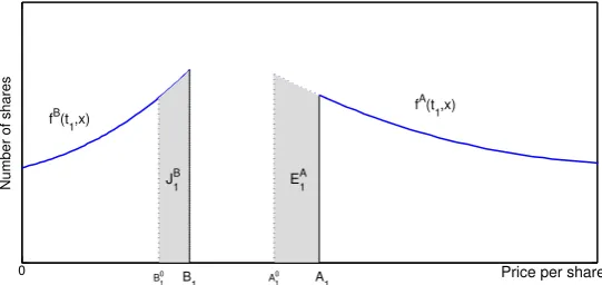
3.1 LOB dynamics with strategy of buyingx0at timet0and then waiting

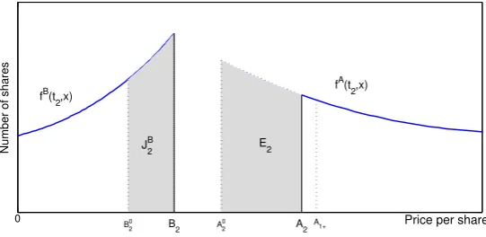
untilt1. . . 53

3.2 Continued LOB dynamics with strategy of buyingx1 at time t1 and

then waiting untilt2. . . 54

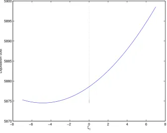
3.3 The change of the liquidation cost against the trade size ξ1 at time

t1. The vertical line isξ1 = 0. . . 66

4.1 The change of the minimal cost _C∗ (the star line) of a cross impact

LOB model against the cross impact resilience rate β. . . 88

4.2 The optimal execution strategies for buying 50 shares on a regular

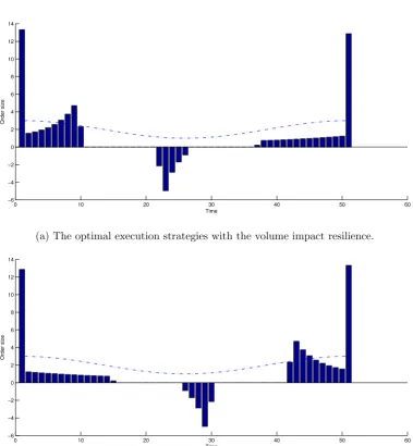
time grid with the volume and price impact resilience. . . 89

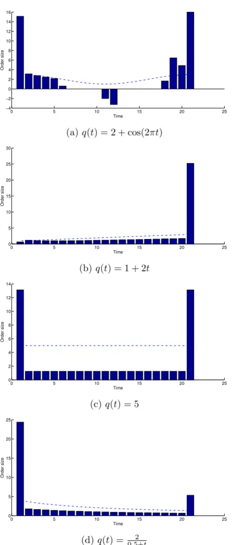
time grid with four diﬀerent depth functions q(t). . . 90

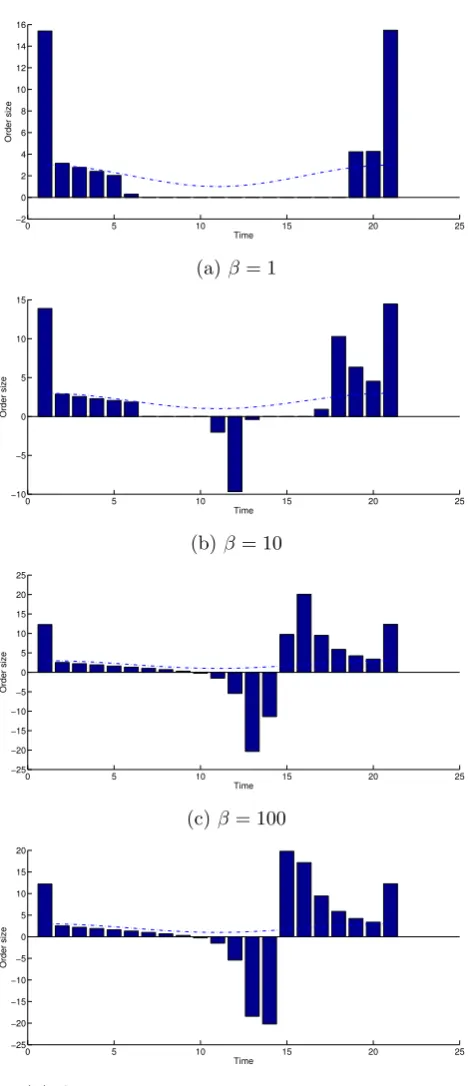
time grid with four values of cross impact resilience rate β when

(10)

time grid with four values of cross impact resilience rate β when

q(t) = ₀_.₅₊2 _t. . . 92

4.6 Optimal execution strategy to buy 50 shares on a regular time grid,

withT = 1, N = 50. The dashed lines are the plot of shape functions. 94

time grid withN = 20 and N = 80. . . 133

time grid withT = 1 and T = 5. . . 133

5.3 The change of the cost function against t2 when t1 = 0.2, q(t) =

q(0)eαt withq(0) = 2, α= 3, ρ= 1,β _{→ ∞} andm= 50/3. . . 141

5.4 The ask side price impact (left) and the bid side price impact (right)

dynamics on time interval [0,1] with t1= 0.2 and t2= 0.4. . . 143

5.8 The change of the cost function against t2 with β → ∞ (left) and

β= 15 (right) when t1. . . 145

dynamics on time interval [0,1] with ρ= 1 andβ = 15. . . 145

5.12 The change of the cost function against t2 when t1 = 0.2, ρ = 1,

(11)

5.13 The phase portrait of the coupled system of ask side price impact

(12)

List of Tables

(13)

Chapter 1

Introduction

In section 1.1, we will briefly review the existing literature about the optimal

trading order execution problem, the concept of limit order book (LOB), market

impact models and the market microstructure underlying these models. Moreover,

we will also provide some brief review on the regularity problem of market impact

model and the resilience eﬀect of the LOB market. Since our research is conducted

on the limit order book structure, some notions about the order book trading will

be introduced in section 1.2. These notions are used throughout this thesis. Then

in section 1.3, we would like to present the motivation of this research. Finally, in

section??, we will give the structure of this thesis and our main contributions.

1.1 Literature review

1.1.1 Optimal trading order execution problem

With or without private information, there are some cases in which a trader

needs to liquidate a large amount of some asset. As proposed in Brunnermeier and

Pedersen [19] some examples are hedge funds with margin calls, traders who uses

(14)

seller who may need to respond to the price increases1_{. Because of the limited}

liquidity in the financial market, trading a large amount of any asset has an impact

on its prices, and usually this price shift is against the trader’s interest. This trading

incurred price shift is called theprice impact.

The basic observation is that the costs of the price impact of a large trade

can be reduced significantly by splitting the large trade into a sequence of smaller

trades. To this end, we adopt the view of Bertsimas and Lo [13] and Gatheral

[33] about the order execution process. They suggested that the trading process

is separated into three layers: The first layer is calledmacro-trader and this layer

decides about the timing of trading and about the order sizes; The second layer

called micro-trader. Given a slice of the order placed by the macro-trader, the

second layer decides whether to place market orders or limit orders. If a limit order

is placed, at which price to trade; The third layer is thesmart order router. Here a

decision is made about which trading venue to send the orders to.

Although it is desirable to have an integrable model for all layers of the

trading process, such a model might be overly complex as suggested in Bertsimas and

Lo [13]. Themarket impact models we consider in this thesis are models developed

for solving the first layer optimal execution problem. We will review the market

impact models in detail in the section 1.1.2. Apart from the market impact models,

there are other first layer related studies focusing on optimal trading times, such as

Kharroubi and Pham [51] and Lehalle et al. [59], or the studies focusing on order

split between transparent and hidden, such as Buti and Rindi [20], Cebiroˇglu and

Horst [22], Esser and M¨onch [29] and Kratz and Sch¨oneborn [55]. The second layer

execution usually involves limit order placement, such as Avellaneda and Stoikov

[10], Bayraktar and Ludkovski [11], Gu´eant and Lehalle [41], Gu´eant et al. [42],

Harris [45], Hollifield et al. [47], Kovaleva and Iori [54]. There is also some research

which combines both the first and the second layer, for example Guibaud and Pham

1_{As stated in Madhavan [62], this is the case that ‘issues of how investors trade are decoupled}

(15)

[43], Guilbaud and Pham [44], Huitema [50], Naujokat and Westray [64]. For the

layer of smart order router, one can refer to Cont and Kukanov [24] and Laruelle

et al. [57] and the references therein.

1.1.2 The market microstructure underlying market impact models

The market microstructure endogenously explain the formation of the price

impact, and the motivation of trading activities, etc. To build a both mathematically

tractable and well rounded market impact model, it is desirable to gain a better

understanding of the endogenous market microstructure that underlies the market

impact models. Some recent books and articles, such as Biais et al. [15], Lehalle

[58], Madhavan [62], O’Hara [66], summarised the market microstructure literature

from the aspects of theoretical, empirical and experimental study.

In a market impact model, the relation between the transacted order volume

and the consequent price shift is described by theprice impact function. The price

impact function is an abstract microstructure description of the interactions between

traders and the liquidity in the market. In other words, it does not model the

dynamics of price impact via interactions of trades at a microscopic level as in a

market microstructure model, but emphasise on a direct relation between a large

order and the price dynamics. As in Alfonsi et al. [5], Almgren and Chriss [9],

Gatheral [32] and Obizhaeva and Wang [65], the asset price in a market impact

model is in the form of

St=S0t + Price impact function

where S0 is an exogenously given process to describe the asset price when it is

unaﬀected by the price impact.

Both the unaﬀected price process and the price impact function are required

to be specified in a market impact model. As suggested in Gatheral and Schied [35]

(16)

first generation market impact models distinguish between two price impact

compo-nents, namely thetemporary impact and permanent impact. Thesecond generation

market impact models is based on the subsequently decay of price impact, which

is called the transient impact. In the rest of this section, we will briefly review the

market microstructure that underline the first and the second generations of market

impact models.

The first generation market impact models and dealer market

Madhavan [62] attributes the cause of temporary and permanent price impact

to three types of costs when one trades in a dealer market. On a dealer market,

liquidity is provided by a specialist who is contractually obliged to always stand

ready to buy at quoted bid and sell at quoted ask. Price is determined via the

specialist’s auction and the trader’s bidding.

The temporary price impact reflects the transitory cost of demanding

liq-uidity, such as order handling fee in Roll [72] and inventory cost in Stoll [81]. The

temporary price impact only aﬀects the individual transaction that has triggered it.

The permanent price impact reflects the specialist’s price update based the

information transmitted to the market by the buy/sell order flows. Thus the

perma-nent price impact is due to the costs of being adversely selected by informed traders

as discussed in Easley and O’Hara [28], Glosten and Milgrom [38], Kyle [56]. The

permanent impact does not only influence the price of the current trade but also

the prices of all subsequent trades.

This kind of market impact models are first introduced in Bertsimas and Lo

[13], Almgren and Chriss [9] and Almgren [8]. The framework of Almgren and Chriss

[9] has now been a basis for practical applications used in the financial industry.

Some variants of the Almgren-Chriss framework are:

1. Adapting the optimal execution strategy for various risk criteria, such as the

(17)

[49] and the expected utility maximisation applied in Schied et al. [79] and

Schied and Sch¨oneborn [77].

2. Introducing the optimal adaptive strategy, for example, Lorenz and Almgren

[61];

3. Applying more general unaﬀected price processes, other than the Bachelier

model, such as the geometric Brownian motion applied in the work of Schied

[76] and Gatheral and Schied [34].

The second generation market impact models and LOB market

On a LOB market, there is no designated liquidity provider. Liquidity is

oﬀered in a self-organised way. In other words, any agent can choose, at any instant

of time, to either provide liquidity or consume liquidity. A satisfactory LOB

mi-crostructure model should be able to include the interactions of diﬀerent traders and

explain how the bid and ask prices are aﬀected by the interactions. Particularly in

this thesis, it is desirable to reflect the same side and opposite side resilience eﬀect

in a LOB model.

We list some survey papers focusing on the market microstructure of the

LOB. They are Bouchaud et al. [18], Gould et al. [40] and Parlour and Seppi [68].

Following the view of Abergel and Jedidi [1] on the classification of LOB

microstruc-ture models, two research methods could be outlined. The first method is a game

theory approach, such as Foucault et al. [30], Goettler and Rajan [39], Parlour [67],

Rosu [74] and Rosu [75]. Among these, the eﬀect of asymmetric information on LOB

trading activities is considered in Bloomfield et al. [16], Goettler and Rajan [39],

Harris [45] and Rosu [75]. In such a trading game, traders are assumed to arrive at

the LOB market randomly and trade strategically by endogenously choosing their

trading decisions as solutions to individual utility maximisation problems. The LOB

dynamics is then the collections of equilibrium strategies of all active traders.

(18)

zero-intelligence models, such as Abergel and Jedidi [1], Cont and Larrard [25], Cont and

Larrard [25], Smith et al. [80] and Toke [82]. Zero-intelligence means the focus of this

approach is more on reproducing the mechanics properties of the order book without

assuming the strategic interactions between agents. The arrivals of diﬀerent order

flows are assumed to be independently and identically distributed point processes.

More empirical studies suggest that price impact is transient, but is not

sep-arated into two parts, namely the permanent price impact and temporary price

impact. In other words, an order creates some immediate price impact that

subse-quently decays over time. Bouchaud et al. [17], Bouchaud et al. [18], Potters and

Bouchaud [70], Weber and Rosenow [85], Wyart et al. [87] are among those

empiri-cal LOB studies which support this transient decay idea. Obizhaeva and Wang [65]

adopted the transient price impact with the same side resilience into the market

impact models. In their research, the LOB is defined via a block shaped and time

independent function. The same side resilience factor was defined via a

determinis-tic exponential function. In recent years, there are some research extended the work

of Obizhaeva and Wang [65]:

1. In Gatheral et al. [37] and Alfonsi et al. [6], the same side resilience factor

follows other deterministic functions.

2. In Alfonsi et al. [4], Alfonsi and Schied [3], Predoiu et al. [71] and Alfonsi

et al. [5], the shape function of the LOB is also defined as a time independent

function but not in block shape.

3. In Alfonsi and Acevdeo [2] and Fruth et al. [31], the LOB shape function is

assumed to be a block shaped function but not independent with time.

4. In Fruth et al. [31] and Weiss [86], the same side resilience factor is considered

to be stochastic.

(19)

1.1.3 Regularity of market impact models

The optimisation problem brings us the issue of regularity of a market

im-pact model. A minimal regularity condition is the existence of admissible optimal

execution strategy. This existence of an optimal solution is guaranteed by the

ab-sence of theprice manipulation strategy (PMS) and thepositivity of liquidation cost

(PLC). Moreover, the resulting optimal strategies should be well-behaved. For

in-stance, we do not want to follow a trading strategy that strongly oscillates between

buy and sell since there is usually additional fees for trading market order. This

oscillation strategy can be excluded by the absence of thetransaction-triggered price

manipulation (TTPM) in a market impact model. The notions of these irregularity

conditions of market impact model will be introduced in section 3.3.

However, we should note that these arbitrage opportunities in market

im-pact models are diﬀerent from the arbitrage in derivative pricing models and are

also distinguished from the arbitrage opportunities generated by asymmetric

infor-mation as discussed in Allen and Gorton [7]. So even a martingale assumption on

the unaﬀected price process will not exclude these irregularities in market impact

models.

Huberman and Stanzl [48] initiate the research on arbitrage opportunity in

market impact models and link this to the arbitrage in derivative pricing framework

via so called quasi-arbitrage. They find that the linearity of the permanent price

impact function is a necessary condition for the absence of the PMS. Their results

are further confirmed in transient models of Gatheral [32] and Gatheral et al. [36].

Alfonsi et al. [6] and Gatheral et al. [37] both research on linear transient LOB model

with general decay factor. They find out a necessary condition on the decay factor for

absence of both PMS and TTPM. Alfonsi and Schied [3] and Kl¨ock [52] represent two

extensions of the linear transient impact model. Alfonsi and Schied [3] generalise

their results with the non-linear price impact function. Kl¨ock [52] introduce the

eﬀect of stochastic linear price impact into market irregularity investigation and

(20)

1.1.4 The resilience of the market impact

In this section, we provide an overview of some theoretical and empirical

studies on the order book resilience. In market impact modelling framework, the

resilience means the price impact induced by a large trade can be reduced if extra

time is given for the market to recover. The resiliency in a LOB is quantified in

three respects:

1. Magnitude, i.e. how much will the best bid or ask price recover.

2. Speed, i.e. how quick will the best or ask price recover.

3. Direction, i.e. same side resilience or opposite side resilience2.

In particular, we will have a discussion on the same side and opposite side resilience

after a trade incurs price impact.

Theoretical studies on the resilience of the market impact

The resilience study in Bouchaud et al. [17] and Bouchaud et al. [18] is

conducted via analysing the diﬀusive behaviour of mid-price (average of the best

bid price and the best ask price) process. They claim that the market observed

mean-reverting mid-price process holds if and only if the price impact decays slowly.

They oﬀer the rational behind price mean-reverting as: the liquidity provider needs

to close their position at a later time without trading at a much higher price. So

the liquidity provider needs to mean-revert their limit order prices after a large

order. The recovery direction is not clarified and their view about the time scale of

resilience is that the mean reversion cannot take place too quickly.

Via a study on high frequency (HF) trader’s optimal market making (i.e.

supplying liquidity with limit orders) strategy, Cartea et al. [21] oﬀer evidence on

opposite resilience in a LOB market on short time scale. The optimal solution

implies that the HF trader should correct the market making strategy in order to

(21)

mitigate the risk of being adverse selected, and exploit the short-term mid-price

deviation via directional strategy. In other words, after a large market buy order,

the HF trader posts further away from the mid-price on the ask side (avoid being

adversely selected) and puts closer to the mid-price on the bid side (exploiting the

short-term deviation by directional strategy). That is to say, HF market maker’s

directional strategy supports the opposite side resiliency of the order book on short

time scale.

Foucault et al. [30] applied a game theory to study continuous-time order

submission problem. To measure the resiliency they use two definitions, namely the

reservation spread and the competitive spread. Reservation spread is the smallest

price improvement by which a limit order trader could make a non-negative profit.

Competitive spread is the patient traders’ reservation spread. Resiliency is then

measured as the probability that the spread reverts to ‘competitive spread’ before

the next transaction. They find out that when traders have the same reservation

spread, the resilience is the fastest and when traders are heterogeneous, the more

the patient traders there are, the faster the price impact decays. There is no clear

results about the resiliency direction.

Empirical studies on resilience of the market impact

Ponzi et al. [69] and T´oth et al. [83] are two empirical studies via event study

based on an order book. They both observe a power lay decay of price impact. In

other words, new limit orders are not placed simply in a way that immediately

reverts the spread back to its original value, but they are sequentially placed close

to the current best price and this leads to a slow decay of the spread. However, the

study of Ponzi et al. [69] does not distinguish the resilience between the same side

and the opposite side recovery. T´oth et al. [83] separately measure the number of

queuing orders on each side of the order book before and after a large market order.

They show for price drop on the bid side the number of queuing limit buy orders

(22)

number of queuing limit sell orders increases and even stays very high for a long time

after the event. That is just the two-side resilience eﬀect which will be explained in

more detail in next section.

Another two important empirical study on order book resilience are: Biais

et al. [14] and Degryse et al. [27]. Biais et al. [14] find new in-spread limit orders

on the ask (bid) side of the market are particularly frequent after large market sell

(market buy) orders. This empirical observation is an evidence of opposite side

resilience. They attribute the co-movement eﬀect to information, in the sense that

part of the resilience in the same side could be mechanical, but the resilience in the

opposite side is believed to be due to the information arising from the shift in the

expected fundamental value. Degryse et al. [27] extend the work of Biais et al. [14]

by studying not only the next incoming limit order after the large market order but

also the sequential orders. They conduct a descriptive event study and they observe

that for small stocks the best ask price jumps up after a large market buy order,

while the best bid price increases as well but without a jump. So does after a large

market sell order. The resilience of two sides of the order book are diﬀerent to the

same large market order..

1.2 LOB and its execution rules

In most of the published literature on LOB, the following terminology has

been adopted. They will be widely used in this thesis too.

Market order and limit order

A limit order is an order to buy or sell some specified quantity of an asset

at a price specified by the trader. It is not executed immediately, instead it enters

the queue of outstanding limit orders. A market order of a given size is an order

that results in an immediate execution at the best available price upon submission.

(23)

explicitly specifying a trading price. Market order is executed against the existing

limit orders. This is the interaction between market and limit orders.

Large order and child order

According to an empirical paper Biais et al. [14], trades are distinguished

by trading direction (buy or sell) and aggressiveness (patience for order execution).

The most aggressive order is placed via a market order to trade a large quantity of

shares which usually demand the execution of more limit orders than that available

at the best price.

In market impact models, a large order corresponds the most aggressive order

in market. In particular, it specifies a large amount of shares which is needed to

be split into smaller orders, so that the adverse price impact incurred by it can be

reduced. This sequential smaller order is called the child order.

Bid side and ask side

A LOB for a single asset is the collection of all active buy and sell limit orders

with the corresponding prices and volumes information. We call the collection of

limit buy orders thebid side of the LOB and the collection of limit sell orders the

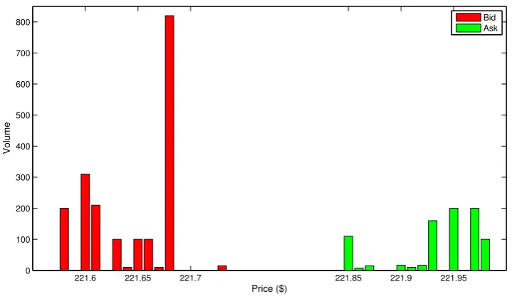
ask side of the LOB. A snapshot of an order book is shown in Figure 1.1.

Order execution rules

Execution of outstanding limit orders by market orders is settled according

to a set of priority rules. Prevailing ones are price-time rule and pro-rata rule.

In this thesis, it is assumed that the LOB follows the price-time priority

rule. Price-time priority LOB markets give priority to orders submitted at more

competitive prices and to displayed orders over hidden orders at the same price level.

(24)

221.6 221.65 221.7 221.85 221.9 221.95 0

100 200 300 400 500 600 700 800

Price ($)

Volume

[image:24.595.147.507.132.342.2]

Bid Ask

Figure 1.1: A LOB Snapshot of AMZN on June 21, 2012.

first-come-first-serve basis. As a result, the price-time priority order execution rules

are:

1. When a market buy order arrives, limit sell orders in the ask side of the

LOB are executed, starting from the orders with the lowest price to the more

expensive ones until the total number of shares ordered is reached.

2. When a market sell order arrives, limit buy orders in the bid side of the LOB

are executed, starting from the most expensive orders to the less expensive

ones until the total number of shares ordered is reached.

Discrete price grids

In a real LOB, orders are placed at a pre-fixed discrete price grids. The grid

step is the smallest interval between two prices and it is called the tick size. The

(25)

LOB dynamics and order flow

The order book evolves over time according to the arrival of new orders. The

price is therefore the result of the interactions between the order book and order

flow. The dynamics of the LOB would be mainly aﬀected by the following four order

flow processes, namely market orders, limit orders placed in the bid-ask spread, limit

orders placed at prices worse than the best price and cancellation of limit orders.

Same side resilience and opposite side resilience

The same side resilience describes the following market situations:

1. After a market buy order, the ask side of the order book will be recovering to

its original status.

2. After a market sell order, the bid side of the order book will be recovering to

Likewise, the opposite side resilience describes the following market

situa-tions:

1. After a market buy order, the bid side of the order book will be recovering to

2. After a market sell order, the ask side of the order book will be recovering to

In terms of order flow, the same side resilience means that:

1. After the arrival of a market buy order, there are new incoming limit sell

orders placed within the current bid-ask spread.

2. After the arrival of a market sell order, there are new incoming limit buy

(26)

1. After the arrival of a market buy order, there are new incoming limit buy

2. After the arrival of a market sell order, there are new incoming limit sell orders

placed within the current bid-ask spread.

Two sides resilience means that, after the arrival of any market order, there are new

incoming limit buy and sell orders placed within the current bid-ask spread.

1.3 Motivations

As demonstrated in the section 1.1.4, empirical evidences of the same side

and opposite side resilience of the market impact are discovered in trading actives.

We believe that these resilience eﬀects are important academically and practically.

But because of the complexity of these features, they are still not well researched. In

Rosu [74], a microstructure LOB model is provided and to the best of our knowledge,

among other LOB models, this model can theoretically replicate the eﬀect of

two-side market impact resilience due to its mathematical tractability.

Diﬀerent from the microstructure LOB model provided by Rosu [74], a

mar-ket impact model based on the LOB is introduced by Obizhaeva and Wang [65]. As

reviewed in the last part of the section 1.1.2, the work of Obizhaeva and Wang [65]

is very popular in recent years and there are various modifications or generalisations

conducted by other academics. However, all these studies did not consider two sides

resilience. Usually, they simplify their models by zero-spread assumption or focusing

on only one-side of the order book.

This thesis fills a gap in literature by providing a mathematically rigourous

proof for the existence of the same side and the opposite side resilience in the

microstructure LOB model of Rosu [74]. Moreover, to the best of our knowledge,

there is no published evidence which examines the eﬀects of the two sides resilience

(27)

considering two sides resilience eﬀects with a non-zero bid-ask spread under the

Obizhaeva and Wang [65] market impact model.

After providing a generalised Obizhaeva and Wang [65] market impact model,

which we call a cross-impact LOB model, research on the optimal execution problem

and the market regularity issues under this model is conducted for two reasons.

Firstly, Kl¨ock [52] and Fruth et al. [31] claimed, but did not prove, that the market

impact models with zero bid-ask spread has weaker regularity conditions than the

models with a non-zero bid-ask spread. So, we would like to verify this argument

in our cross-impact LOB model. Secondly, we want to investigate the eﬀects of two

sides resilience on the first layer optimal execution strategy, which has long been

(28)

Chapter 2

Resilience in LOB

microstructure model

In this chapter, our aim is to show the presence of same side resilience and

opposite side resilience in an order book market. We base our analysis on a game

theoretical model given by Rosu [74]. Compared to other game theoretical models

summarised in Section 1.1.2, there are several reasons to work on the model of

Rosu [74]. First, it allows for a flexible spread of the order book and for explicit

measurement of resiliency with enough mathematical tractability, compared to the

models of Parlour [67], Foucault et al. [30] and Goettler and Rajan [39]. Second, the

direction of the resilience is able to be reflected and modelled in this model, while

it is assumed a fixed one tick size spread in Parlour [67]. Third, the motivation

of trading is exogenous to the model, namely the eﬀect of asymmetric information

is not modelled. Rosu [75] provides an alternative model in which the information

eﬀect is considered. Fourth, it includes the execution time risk of limit orders into

the model formulation, as in Foucault et al. [30].

In Section 2.1 we summarise the model of Rosu [74]. It starts by reviewing

the main characteristics of this continuous time trading game proposed in Rosu [74].

(29)

in the one-side book case, since this case is quite intuitive and admits closed-from

equilibrium strategies. It turns out that the properties of one-side case can be easily

extended to the two-side case.

We present our main results in Section 2.2. In Section 2.2.1 we reinterpret

the same side resilience and opposite side resilience by notions of Rosu [74]’s trading

model. The same side resilience is reflected by the positivity of the diﬀerence between

same side temporary price impact and permanent price impact caused by a same

side market order. The opposite side resilience is measured by the positivity of the

non-execution side permanent price impact. This is an essential step since the price

adjustment in this continuous time trading game is taking place instantaneously,

while the transient resilience is a time-dependent feature of a LOB. Section 2.2.2

deals with the solutions of the Markov equilibrium obtained in the one-side order

book case. We present the solution structure in our Proposition 2.2.2 which is

distinguished from the results of Rosu [74]. In Section 2.2.3, we provide a rigourous

proof of the same side resilience by looking at the asymptotic behaviour of the

price impact functions under the assumption of fast decay arrival rates. We also

construct a counterexample of the same side resilient in Proposition 2.2.4 where the

fast decaying assumption did not hold. Section 2.2.4 reproduce the results in Rosu

[74] about the opposite side resilience in this LOB model.

2.1 The model description

2.1.1 Characteristics of the LOB trading game

The limit order book is of one asset with no dividend. The game is happening

on time interval [0,∞), and trading takes place in continuous time1. The tick size

of price grid is zero, i.e. the prices can take any real value. We take the reason to

trade for all traders to be exogenous to the model. All information about the order

1_{Since there is no universally accepted model of continuous time stochastic game and related}

(30)

book and trader strategy are publicly available. Traders can choose between market

order and limit order. The execution of limit orders is subject to the price-time

priority rule as discussed in the Section 1.2. The limit order can be cancelled or

revised at will with no cost. After order execution, the agents exit the order book

forever. There is no delay in trading, in the sense that submitting or execution

happens instantaneously.

The players form a countable set. They are distinguished by the patience

and trading directions of buy or sell. More precisely, there are four types of traders

considered here: patient buyer, patient seller, impatient buyer, and impatient seller.

Each player’s choice of buy or sell, patience and amount of trading orders are

ex-ogenously given outside of the model and stay the same during the trading game.

For simplicity, it is assumed that the impatient traders only submit market order,

which is automatically executed against existing limit orders. Patient traders choose

strategically between market and limit order and the price to submit if a limit order

is used. The price of a limit sell order, PS, and the price of a limit buy order, PB,

is constrained to lie between [P , P]. Moreover, it is assumed that there is an infinite

supply (demand) at priceP (P) which is provided exogenously. Patient traders

ar-rive with only one unit to trade. Impatient traders can submit up tok-unit market

orders for some constantk_≥1.

The arrivals of traders at the order book are modelled according to

indepen-dent Poisson processes with constant, exogenous intensity rates. Denote the arrival

rates for diﬀerent type of traders as following:

                    

Fori_≤k,µi>0 is the arrival rate of i-unit impatient buyer. Ifi > k,µi= 0;

Fori≤k,λi >0 is the arrival rate ofi-unit impatient seller. If i > k,λi= 0;

µ >0, arrival rate of patient seller;

λ >0, arrival rate of patient buyer.

(31)

wait-ing costs. More specifically, the utility function for market order traders is the

instantaneous best prices at the submitting time, since they do not need to wait for

execution. The expected utility functions for limit order seller and buyer at time

t∈[0,∞) are defined respectively as

f(PS, t) :=Et[PS−r(τ −t)] and

g(PB, t) :=−Et[−PB−r(τ−t)],

whereτ > t is the random execution time andr is the waiting cost discount factor

for patient agents. That is, limit order traders bear the execution time risk. There

are a few things we should note about these utility functions. First,−g represents

the expected utility of a buyer since the higher utility is obtained for a buyer by

lowering the price to pay. The sign ‘−’ was moved to the right hand side so that it

is convenient to maximise bothf and g for buyer and seller at any time. Second,

by assuming a linear relationship between the execution price and the discounted

waiting cost, there is possibility that the utility becomes negative. One could instead

consider an alternative form of utility functions

f(PS, t) :=E�SP e−r(τ−t)�

and

f(PB, t) :=E�PBe−r(τ−t)�.

However, the model is already too complicated to add more complexity from the

utility function. To this end, we can always choose the waiting cost discount factorr

such that the utility is positive. In fact, we will see in the sequel that in equilibrium

the utility has a positive constant lower bound.

The players can respond immediately in this continuous time trading setting.

In other words, the trader will keep the current order as long as the other agents

(32)

timet, this trader will immediately undercut her order price att.

2.1.2 One-side order book game

In this section, we will consider firstly one-side of the order book. Without

loss of generality, we focus on the ask side of a LOB. For the ask side, the best bid

price is the reservation value of the limit order sellers, as they can always submit a

market sell order at the best bid price and exit the trading. So we set the lowest

priceP to be the best bid price for sellers.

For description simplicity, we set Σ := lim

k→∞

�k

i=1µi and introduce the

fol-lowing notations:

m: the number of limit order sellers in the order book;

am(i): the ask price of the ith limit sell order counted from the best ask price, in

an order book withm limit order sellers withi= 1, ..., m;

am: the best ask price for am limit order seller order book.

Firstly, we review the construction of the competitive Markovian equilibrium

in Rosu [74]. At the beginning, the order book is empty, i.e. m= 0. At some timet

patient seller 1 comes and places a limit order at the maximum price levela1 =P.

This is required by the Nash equilibrium since P is the highest price as long as

seller 1 is the only one in the order book. Suppose then a second patient seller 2

arrives. If immediate response is not allowed, seller 2 would secure earlier execution

by placing a limit order ata2 =a1−δ for some very smallδ >0. The limit order of

seller 2 gets executed before that of seller 1 with only infinitesimal price sacrifice, the

expected utility of seller 2 is strictly higher than that of seller 1. However, seller 1 is

allowed to undercut his limit order instantaneously toa1−2δ. So a price war would

follow. As the limit order price gets undercut, the utility for both of them decreases.

Therefore, in equilibrium, seller 2 should submit a limit order ata2< a1 =P such

(33)

The same idea works for m-seller order book as well. In equilibrium, the

sellers have their limit orders placed at diﬀerent prices but get the same expected

utility; otherwise, they would be undercut by each other. The same-utility property

reflects the assumption that the seller with a higher limit order price needs to wait

longer. As a result, we could show that in equilibrium the utility of limit order seller

depends only on the number of active sellers in the bookm. Thereafter, we denote

the seller’s expected utility byfm. Since the arrival of patient sellers is modelled by

exogenously given independent Poisson processes, the state variablemis exogenous

and follows a Markov process. According to the definition of Markov strategy in

Maskin and Tirole [63], the state m utility function fm and the trading strategy

form a Markovian perfect equilibrium.

Apart from determining the price strategies in equilibrium, we also need to

know how limit sell order traders revise their orders when someone in the book

deviates. To this end, Rosu [74] applied the notion of competitive2 equilibrium,

in which a local deviation from one trader can be stopped by any other trader’s

immediate undercutting, assuming that the rest of the equilibrium does not change.

The features of large amount trader and instantaneous response make the choice of

competitive equilibrium natural3.

Then we consider some properties of the utility functionfm, i.e. the boundary

conditions offm. We should note that the state variablemis the only state member

and must be finite. Supposem_{→ ∞}, the expected execution time for the top seller,

i.e. the seller with the highest ask price, would beE[τ]→ ∞. Hence the top seller’s

expected utility isE[am(m)−r(τ−t)]→ −∞. Instead, the top seller could at least

improve her trading by submitting a market order with priceP which gives him the

reservation utility.

2_{An example of non-competitive equilibrium is given in the NASDAQ dealer market study by}

Christie and Schults [23].

3_{By Rosu [73], an Markovian equilibrium is competitive if a restriction of the strategies on time}

interval (t, t+δ) is still a Markov equilibrium. This restriction can be made because of the Markov

(34)

In addition, from the economic point of view, we obtain that the expected

utility functionfm decreases withmand the best ask priceamis decreasing withm

(since more limit order sellers incur longer waiting time). Meanwhile, the minimum

value of a limit sell order should be no less than the reservation valueP. In other

words, when the utility of waiting till execution is less than the utility of submitting

a market sell order at P(recall that P is defined to be the best bid price), some

seller would just cancel their limit orders and place market orders at P. Then

it is reasonable to define a maximum capacity M := max{m : fm ≥ P}4 and a

mixed strategy in which limit order trader randomly switches to a market order

with Poisson(ν). There are four types of mixed strategies that could happen when

there are M sellers. These are introduced in Proposition 12 and Corollary 2 in

Rosu [74]. In particular, the notion of rigid equilibrium is constructed here. Rigid

equilibrium means that if some agents have mixed strategies, mixing is done only

by the agents with the most competitive limit orders (highest bid or lowest ask).

Then, we derive a recursive system of utility functions fm to compute the

equilibrium strategy. For a book of m < M sellers in equilibrium, the market can

go to: statem+ 1 if a new limit order seller arrives with probability _µ_+Σµ , or to state

m−iwithi= 1, ..., kif an i-unit market order buyer arrives with probability µi

µ+Σ,

where Σ =�µi. Apart from this, patient sellers lost utility in a way proportional

to expected waiting time with discount factorr. One obtains the formula

fm =

µ

µ+ Σfm+1+

k

�

i=1 µi

µ+ Σfm−i− r

µ+ Σ.

Furthermore, we construct the individual limit sell order prices am(i) for i =

1, . . . ,min_{m, k_}. With rate µi, an impatient buyer arrives and places an i unit

market order. Theith seller will receivesam(i). The non-executed sellers will have

4_If_f

M < P, some of the sellers could always improve their utility by submitting a market order

directly at priceP and get a better utilityP > fM. This is a contradiction with the optimisation

of each trading strategy. IffM > P, let us consider what happens in stateM + 1. If one agent

acceptedh=P at some time and exited the game, the utility of the other agents would befM > P.

The utility for the agent who acceptshis lower thanfM. So no seller would accepthand everybody

(35)

the same utility which is equal to fm−i with probability µi_Σ. Since all sellers must

have the same expected utility in equilibrium, theith price in am-seller order book

am(i) must be equal to the expectation of all possible utilities, i.e.

am(i) =

�

j≥iµjfm−j

�

j≥iµj

. (2.1.1)

Define by convention thatfi =P fori≤0.5

When the order book reaches its maximum capacityM, the arrival of a new

patient seller does not aﬀect the state of the order book since in equilibrium the new

arrival will immediately place a market order at priceP and exit. With probability

µi

ν+Σ an i-unit market order buyer arrives, the system would go to state M−i. Or

with probability _ν_+Σν the bottom seller, i.e. the seller with the lowest ask price,

switches to a market order atP and exits by the rule of rigid equilibrium. Similarly

one obtains a formula for stateM utility, which is

fM =

ν

ν+ ΣfM−1+

k

�

i=1 µi

ν+ ΣfM−i− r

ν+ Σ.

Theorem 2 in Rosu [74] provides the strategy in equilibrium: ifm= 1, then place a

limit order ata1(1) =P; Ifm= 2, ..., M−1, look at the bottomklevels (or at allm

levels ifm < k), which aream(1), ..., am(k). If any of them is not occupied, occupy

it. Anything aboveam(k) does not matter; if m =M, the strategy is the same as

form = 2, ..., M ₋1, except for the bottom seller at aM(1), who exits (by placing

a market order atP) after the first arrival in a Poisson process with intensityν; If

m > M, then immediately place a market order at P. The equilibrium is unique

in the class of rigid equilibria, in the sense that any other rigid equilibrium leads to

the same evolution of the state variables.

5_{This can be seen by equation (2.1.1) and}_a

1 =P. It is technically required thata1 =a1(1) =

�

j≥1µjfm−j

�

(36)

2.1.3 Two-side order book game

Now we are ready to review the two-side case in Rosu [74], since the derivation

of the opposite-side resilience depends on the knowledge of the best pricesam,n and

bm,n. Similarly as in the one-side case, we will familiarize ourselves with the possible

trading activities, the set of state variables (m, n) wherem is the number of patient

sellers andnthe number of patient buyers in the book, and the recursive system of

utility functionsfm,nandgm,n. Thereafter, if given a solution of the recursive system

off,g, according to Definition 4 in Rosu [74] one can then obtain the formulas for

best pricesam,n andbm,n.

For simplicity in the two-side game, we assume that the impatient traders

can only submit one-unit order, i.e. µi = 0 andλi = 0 if i >1, and will denote by

m: the number of limit order sellers in the order book;

n: the number of limit order buyers in the order book;

am,n: the best ask price in a mlimit sell and nlimit buy order book;

bm,n: the best bid price in am limit sell andn limit buy order book.

For illustration, let us see the trading activities for example at state (1,0).

The market may go to:

(0,0) if either an impatient buyer arrives after time T1 ∼ exp(µ1) and buy with a

market order at pricea1,0 =P, sincea1,0 =P is the highest possible sell price

to achieve for the patient seller in the range [P , P]; or after some random time

T2 ∼ exp(λ) a patient buyer arrives and submits a limit buy order at price

h. The existing patient seller accepts to trade at h if the expected utility

of waiting till next arrival of a new agent is less than h according to the

Proposition 12 in Rosu [74].

(1,1) if after some random timeT2 ∼exp(λ) a patient buyer arrives and submits a

(37)

patient buyer stays and behaves as a monopolist at the bid side by changing

bid price fromh to a lowest buy price atB immediately.

(2,0) if another impatient seller arrives after time T3 ∼exp(λ1).

As in the one-side case, if an order book with m limit order sellers and n

limit order buyers is in equilibrium, all the m sellers must have the same expected

utility denoted byfm,n, and all then buyers must have the same (minus) expected

utility denoted bygm,n. It is defined that the state region Ω as the set of all states

(m, n) where in equilibrium agents wait in expectation for some positive time. The

state variable m, n are finite because of the same reason as stated in the one-side

case.

Thereafter, we can summarize all possible trading activities. For any state

(m, n)_∈Ω, the system can go to the following neighbouring states:

Activity A: leading to (m−1, n), (1) if an impatient buyer arrives, or (2) if a

patient buyer arrives and place a market order to trade with the bottom limit

order seller at the best ask priceam,n, or (3) if a patient seller cancels the limit

order and submits a market order atP when n= 0;

Activity B: leading to (m+ 1, n), if a patient seller arrives and submits a limit

order;

Activity C: leading to (m, n−1), (1) if an impatient seller arrives, or (2) if a

patient seller arrives and place a market order to trade with the top limit

order buyer at the best bid price bm,n, or (3) if a patient buyer cancels the

limit order and places a market order atP whenm= 0;

Activity D: leading to (m, n+ 1), if a patient buyer arrives and submits a limit

order;

Activity E: leading to (m₋1, n₋1), (1) if the existing bottom patient seller

switches to a limit order at a lower than best ask (bid) price h such that

(38)

by placing a market order; (2) if the existing top patient buyer switches to a

limit order at a higher than best bid price h such that h =fm,n =gm,n, and

the existing bottom patient seller immediately accepts it by placing a market

order.

Now we are ready to define the mixed strategies under this two-side case.

First of all, it is observed from Proposition 12 case (1) that it must be fm,n> gm,n

if all traders prefer to wait in the order book. Otherwise, in state (m, n) with

fm,n < gm,n, the patient sellers could improve their utility by placing a limit order

at some price levelh_∈[fm,n, gm,n] and some patient buyer immediately accepts one

of the oﬀers by placing a market order. This is feasible by noting that −gm,n is

the expected utility for buyers. This reflects the fact that as new patient buyers

and sellers arrive, they place limit orders on both sides until it is better oﬀ to trade

immediately rather than wait. In case of state (m, n) with fm,n = gm,n, the order

book is defined to be full and the traders on both sides play a game of attrition. By

Proposition 12 and Corollary 2 in Rosu [74], according to a Poisson process with

intensityνm,n traders on both sides might apply mixed strategies. More specifically,

they are one of the following four cases of mixed strategies: A(3), C(3) and E(1),

E(2). The set of the states (m, n) at which mixed strategies take place is defined as

the boundaryγ of Ω.

In the two-side limit order book, some typical points in Ω can be summarised

as in Figure 2.1, in which the big dots are boundary and small dots are the interior

of the state region. Notations in this figure follow those in Rosu [74]. We should

note that Ω does not have to be that specific shape.

For each point (m, n) in the state region, we can get a coupled system for

fm,n and gm,n and corresponding equations for am,n and bm,n. Recall thatk is the

maximum units that a market order can trade with and r is the waiting discount

factor. For each boundary point (m, n)_∈γ, a corresponding numberνm,n≥0 is the

intensity of a Poisson process with which some traders will have mixed strategies.

(39)

✲ ✻

m n

� � � � � � �

� � � � � �

� � � �

� � �

� �

Type 0 ✲

✻ ✛

Type 2b

✻ ✛

Type 3b ✲

✻ ✛

❄Type 1

✲ ✛

❄ Type 4b ✲

✻

❄

Type 2a ✛

❄ Type 5

✛ ✻

❄ Type 4a ✲

[image:39.595.213.431.119.306.2]

❄ Type 3a

Figure 2.1: Types of points in the state region Ω cited from Rosu [74]. The points

at boundary are types 3a,3b,4a,4b,5. The types 0,1,2a,2b are interior points.

Then define the recursive system associated to (Ω, k, ν) by considering the following

set of equations for each state (m, n)∈Ω .

First, we consider the interior points at which there are no mixed strategies.

If (m, n) is of type 0, as illustrated in Figure 2.1, we have m= 0 andn= 0. Then

we define by convention f0,0 = P and g0,0 = P. If (m, n) is of type 1, there are

four possible trading activities which can aﬀect the state. They are activitiesA(1),

C(1), B and D. One obtains the recursive equations

fm,n=

1

Σ1 [fm+1,nµ+fm,n+1λ+fm−1,nλ1+fm,n−1µ1−r]

and

gm,n =

1

Σ1

[gm+1,nµ+gm,n+1λ+gm−1,nλ1+gm,n−1µ1+r].

If (m, n) is of type 2a, this is the state where there is no existing limit order sellers.

As illustrated in Figure 2.1, we have m = 0. Then set f0,n = P. The arrivals of

(40)

B,Dand C(1). One obtains the formula for g0,n as

g0,n= 1

Σ2

[g1,nµ+g0,n+1λ+g0,n−1λ1+r].

For type 2b, as illustrated in Figure 2.1, we have n= 0. So the recursive equations

under this situation,fm,0 and gm,0, are similar to those for type 2a.

Next, we look at the boundary states when mixed strategies might happen.

If state (m, n) is of type 3a, set by convention f0,n=P. Since the capacity of limit

order buyers reaches its maximum and there is no existing limit order sellers, event

E(2) is not possible butC(3) might happen at priceP. The arrivals of new patient

seller will place a limit order and stay in the book, which implies activity B not

A(1). The arrival of new impatient seller incurs activity C(1). Thus, one get the

formula for limit order sellers’ utility

g0,n = 1

µ+ν0,n+λ1

[g1,nµ+g0,n−1ν0,n+g0,n−1λ1+r].

If (m, n) is of type 4a, existing limit order sellers reach its maximum capacity.

Therefore the limit order sellers will not wait but trade following activityE(1). If a

new patient seller arrives, she will immediately submit a market sell order and trade

with the top limit order buyer atbm,n. This implies that activityC(2) might happen.

If a fnew patient buyer arrives, it is still better to wait than trade immediately for

him. So event D is possible. The trading of impatient buyer and seller will incur

eventA(1) andC(1). One obtains the utility functions

fm,n =

1

Σ1+νm,n

[fm,n−1µ+fm,n+1λ+fm−1,nµ1

+fm,n−1λ1−r+fm−1,n−1νm,n] and

gm,n =

1

Σ1+νm,n

[gm,n−1µ+gm,n+1λ+gm−1,nµ1

(41)

If (m, n) is of type 5, in the case of impatient traders arrival, they trade as normal

with market orders, which are eventsB andD. In the case of patient traders arrival,

the order book is in a state where it is better to trade immediately than wait. So

patient traders will either do E(1), E(2) or do A(2), C(2). Thus, one obtains the

formula

fm,n =

1

Σ1+ 2νm,n

[fm,n−1µ+fm−1,nλ+fm−1,nµ1

+fm,n−1λ1−r+ 2fm−1,n−1νm,n] and

gm,n =

1

Σ1+ 2νm,n[gm,n−1µ+gm−1,nλ+gm−1,nµ1

+gm,n−1λ1+r+ 2gm−1,n−1νm,n].

We can defineam,n and bm,n based on the ideas of the same expected utility

in equilibrium as in the one-side case. More specifically, the one who is getting

executed must have the same expected utility as the other traders in the book on

the same side. They are given by the following formulas:

        

am,n =fm−1,n and bm,n=gm,n−1, if (m, n) is of type 1;

a0,n =P and b0,n =g0,n−1, if (m, n) is of type 2a;

am,0=fm−1,0 and bm,0=P , if (m, n) is of type 2b.

For those points on the boundary, without loss of generality, we will give the

derivation of am,n at state of type 5. There are three situations where the existing

bottom limit order seller gets executed: trade to a market buy order in cases of

A(1), A(2) or do mixed strategy E(1). With probability µ1+λ

µ1+λ+νm,n, the bottom

seller trades to market buy order and receives am,n, while the other limit order

sellers getfm−1,n. With probability _µ₁₊νm,n_λ₊_νm,n, the bottom seller switches to a limit

order at some lower levelh, and the top limit order buyer immediately switches to

(42)

that for both the bottom seller and top buyer not losing utility thanfm,n and gm,n

respectively. So it has to be that h = fm,n = gm,n. All the other sellers now get

utilityfm−1,n−1. The same expected utility for all sellers leads to the relationship

am,n(µ1+λ) +νm,nfm,n =fm−1,n(µ1+λ) +νm,nfm−1,n−1.

Thereafter, we get the formulas

am,n =fm−1,n+ νm,n

λ+µ1

(fm−1,n−1−fm,n) and

bm,n =gm,n−1+ νm,n

λ+µ1(gm−1,n−1−gm,n).

The derivations for other types of boundary points are similar.

Theorem 3 in Rosu [74] gives the existence of a rigid, competitive Markovian

equilibrium in the two-side case. We summarise it here: If (m, n) is in the interior

of set Ω, the bottom seller places a limit sell order atam,n, and the top buyer places

a limit buy order at bm,n. If (m, n) ∈ γ, then the strategy is the same as the one

above, except that with the first arrival in a Poisson process with intensity (νm,n)

the bottom seller changes the limit order from am,n to h = fm,n = gm,n, and the

top buyer immediately accepts it via a market buy order; the top buyer would not

accept any higher limit sell order. If (m, n)∈/ Ω andm, n >0, then the bottom seller

places a limit order at h = fm,n =gm,n and the top buyer immediately accepts it

via a market order. If (m, n)∈/ Ω andn= 0, then the bottom seller places a market

order atP and exists the game.

2.2 Price impact and resilience

We present some of our main contributions in this section, we firstly translate

the definitions of the price impact and the price overshoot in Rosu [74] by notions of

(43)

one-side case, we give a rigourous proof of the theorem 2 in Rosu [74] by introducing the

proposition 2.2.2. Thirdly, we provide a rigourous proof for same side resilience in

the Proposition 2.2.3. Finally, we also provide an counterexample of the conjecture

in Rosu [74], which stated that the same side resilience exists without the restriction

on arrival ratesµi and µ.

2.2.1 Resilience measurement

Recall that the same side resilience is the decay of the price impact on the

same side of the large market order. The opposite side resilience is the decay of the

price impact on the opposite side of the large order.

When ani₋unit market buy order is submitted to the order book ofmlimit

order sellers, this market order clears the sell orders from the lowest one to the

lowestith order. The lowest (i+ 1)th limit sell order immediately becomes the new

best ask order in the order book. This is the immediate price impact incurred by

the large order. Since the agents are fully strategic, they instantly regroup to adjust

to the new state withm−isellers. The second best ask price changes corresponds

to the transit decay of the first price change.

In Rosu’s model [74], these two price changes take place instantaneously,

and are described by the notions of temporary and permanent impact. However,

as stated in Chapter 1, the permanent price impact is observed in the long term

time. To prevent misunderstanding, in this thesis the permanent price impact is

the second price change and the temporary price impact is the first price change

as discussed above. Without loss of generality, we will define the temporary and

permanent price impact on the ask side of the order book. These definitions could

be extended to the bid side in a similar way.

Definition 2.2.1: Consider the limit order book with only patient sellers and

impa-tient buyers who can submit a market order of size at most k-unit for some k >1.

(44)

order starting from the best ask price am(1) for j≤m. Denote byi0:= min{k, m}.

The temporary price impact on the ask side caused by a buy market order of size

i_≤i0 is defined as the diﬀerence

I_mA(i) :=am(i+ 1)−am(1), (2.2.1)

which is the diﬀerence between the i+ 1�st oﬀer am(i+ 1) from the bottom and the

best ask price am(1).

The permanent price impact on the ask side caused by a buy market order of

sizei_≤i0 is given by

P_mA(i) :=am−i(1)−am(1), (2.2.2)

which is the diﬀerence between the best ask price am−i(1) in the state with m−i

sellers and the best ask price am(1)before the market order was submitted.

If use the superscription A for the ask side and B for the bid side, we say

there is the same side resilience if the diﬀerence between same side temporary impact

and permanent impact is positive, i.e. IA

m(i)−PmA(i) > 0 and ImB(i)−PmB(i) > 0. The opposite side resilience is measured by the positivity of the opposite side, or

non-execution side, permanent impact, i.e. PB

m(i) >0 if ImA(i) is non-negative and

P_mA(i)>0 ifI_mB(i) is non-negative.

2.2.2 Solution of the recursive system in the one-side case

In this part, we will discuss the properties of the solution of the recursive

system proposed in the one-side order book case. This is an important step in

proving the same side resilience and opposite side resilience. In general, it is diﬃcult

to get an explicit solution of the coupled recursive system in the two-side case.

Consider the limit order book with only patient sellers and impatient buyers who

Limit order book resilience and cross impact limit order book model

University of Warwick institutional repository: http://go.warwick.ac.uk/wrap

A Thesis Submitted for the Degree of PhD at the University of Warwick

http://go.warwick.ac.uk/wrap/67146

This thesis is made available online and is protected by original copyright.

Please scroll down to view the document itself.

Limit Order Book Resilience and Cross

Impact Limit Order Book Model

Xin Geng

Mathematics

Declaration

Acknowledgements

Abstract

Contents

List of Figures

List of Tables

Chapter 1

Introduction

1.1

Literature review

1.2

LOB and its execution rules

1.3

Motivations

Chapter 2

Resilience in LOB

microstructure model

2.1

The model description

2.2

Price impact and resilience