Bosonic loop soups and their occupation fields

(1)

A Thesis Submitted for the Degree of PhD at the University of Warwick

Permanent WRAP URL:

http://wrap.warwick.ac.uk/81891

Copyright and reuse:

This thesis is made available online and is protected by original copyright.

Please scroll down to view the document itself.

Please refer to the repository record for this item for information to help you to cite it.

Our policy information is available from the repository home page.

(2)

Bosonic Loop Soups and Their Occupation

Fields

by

Owen Daniel

Thesis

Submitted for the degree of

Doctor of Philosophy

Mathematics Institute

The University of Warwick

September 2015

M A E

G NS

I T A T MOLEM

U N

(3)

Acknowledgements

First and foremost I would like to thank my supervisor Stefan Adams for his sup-port of my work, his enthusiasm and knowledge. Thank you also to David Brydges for generously sharing his time and thoughts with regards to my project, in addi-tion I would like to thank him and the rest of the mathematics department at the University of British Columbia for organising my multiple visits to Vancouver. I am also grateful for the support and advice of many members of sta↵ at the Warwick Mathematics Institute. I thank Xue-Mei for her blend of wisdom and humour, Nikos for his words of encouragement, and Carole for her dedication to all of us graduate students.

I have been fortunate enough to spend the last four years in the company of many good friends. I am particularly indebted to my friends in Vancouver: thank you for making me feel like a local during what could have been three rather lonesome months... and for enduring the numerous raccoon and beaver spotting expeditions. In my previous MSc thesis I thanked Simon Bignold for driving me home in the snow; this time around I would like to acknowledge his excellent taxi services, provided at 3am one December morning. Without him I would not have been able to take my bike on holiday. I would also like to mention my lunch time sparring partner Ray: the final few months of the PhD have not been the same without my bastion of morality to quarrel with over a punnet of tomatoes. Thanks go to Sergios, in part for his mathematical thoughts, but primarily for his company as a rather arduous training partner on cold and sunny days alike. Also thanks to Tejay, Ryder and Fausto for making this journey possible.

(6)

Declarations

The work in this thesis was conducted by the author during the period October 2012 - September 2015 at the University of Warwick, in collaboration with Dr Stefan Adams. Elements of the introduction were previously used in my Masters theses [Dan11, Dan12]. Where we make use of work not our own, or rework established arguments, we write (for instance): “we follow [Szn12], p.13”.

(7)

Abstract

(8)

List of Notation

Mathematics

[N] The set of integers 1,2, . . . , N.

R+ Positive real numbers.

R Negative real numbers.

H Negative half plane. Spec(A) Spectrum ofA.

@ Multi-subset.

# Cardinality of a discrete set. Re,Im Real and imaginary part.

SN Symmetric group on [N]. Probability

1

_{A} Indicator variable of an eventA.

(d)

= Equality in distribution.

(d)

! Convergence in distribution. a Dirac -measure ata.

M1 Space of probability measures on

a measure space. Statistical Mechanics

Inverse temperature.

h Chemical potential.

Z⇤( , N) Canonical partition function .

⌅⇤( , h) Grand canonical partition

function.

⇢c( ) Critical density.

˜ 1-particle reduced density ma-trix.

Graph Theory

(⇤, w,) Weighted graph. Rate vector.

P (Sub)-stochastic transition ma-trix.

P,E Law and expectation of a random walk.

lT

x, lx Local time atx.

m⇤ Spectral measure.

Loop Models

( ,G) Measure space of loops.

µh Markov loop measure.

µB

,h Bosonic loop measure.

P,E Law and expectation of the Markov loop soup.

PB_,_EB _{Law and expectation of the} Bosonic loop soup.

L Occupation field of a Poisson loop soup.

L Mean occupation.

n= (n(j)_)j

1 Cycle distribution.

⌦=RZd

Space of fields onZd_. T,TN Continous and discrete torus.

(9)

Introduction

Statistical mechanics can be summarised as the study of macroscopic models via a microscopic description; that is, we define a model locally (on the micro-scale) and study global (or macroscopic) changes as we vary some model parameters. To motivate this description we turn to perhaps the best known model of statistical mechanics, the Ising model. This is a model for magnetism, where the polarity of any particular site in a material is assumed to be influenced by nearby sites. In the presence of a strong external magnetic field the polarity of the sites align and the material is considered to be magnetized, moreover there is long-range correlation between sites. As the strength of the external field reduces to zero, intuition suggests that this long-range correlation should also vanish to 0. This, however, is not always the case: depending on the model temperature the material can retain a magnetic force even in the absence of an external field, seen by the continued presence of long-range correlations. This is an example of a phase transition, where for one long-range of the parameters we see typical behaviour whilst for another range we see other behaviour entirely (in this case above the critical temperature there is no residual magnetism, whilst below it there is). Defining and proving the existence of phase transitions is of central importance to the study of statistical mechanics.

In the instance of the Ising model the search for a phase transition was first under-taken by Ising [Isi25] who showed that in the 1-dimensional model no such phase transition occurs. It would take the best part of two decades before Onsager [Ons44] provided the first proof that the Ising model in 2-dimensions does undergo a phase transition, and provided an exact solution for the critical temperature for the near-est neighbour model on the square lattice. Onsager’s work is seen by many to be the starting point of the rigorous mathematical study of phase transitions, and to this day the Ising model remains one of the most studied models of statistical mechanics. At the same time as Ising was working on his eponymous model1, a di↵erent type of phase transition was being proposed by physicists Satyendra Nath Bose and Albert Einstein. They considered a gas of particles distributed in a box, where each particle is considered to be at a certain energy level. Einstein [Ein24] defined a model in which there was no particle interaction, and observed that at moderate temperatures

1_{That the model takes Ising’s name is somewhat contentious since the model was first proposed}

(10)

only a microscopic proportion of the atoms were designated to any given energy state; however, given a low enough temperature a macroscopic proportion occupied the lowest of the energy states, the ground state. Einstein remarked: “A separation is e↵ected; one part condenses, the rest remains a ‘saturated ideal gas’.” Unlike the Ising model, where the physical phase transition was known to be exhibited in real magnets well before the mathematical phase transition was proven to occur, prior to Einstein’s observation nobody had considered that such a condensation phenomenon could occur, and for some time little attention was paid to the problem. It was only after London [Lon38] observed that a similar transition occurs in liquid helium that Einstein’s suggestion was given its due attention. Even then the occurence of this transition, which had now become known as the Bose–Einstein condensation phenomenon, remained a purely theoretical construct. It was not until 1995 that this would change. With the advent of new cooling technology two independent teams demonstrated the existence of the Bose–Einstein condensate: the group of Eric Cornell and Carl Wieman condensed a vapor of rubidium 87 atoms [CW02], and shortly after Wolfgang Ketterle’s team condensed a gas of sodium-23 atoms. The breakthroughs of these two groups lead to all three physicists being awarded the 2001 Nobel Prize for Physics dedicated to “the achievement of Bose–Einstein condensation in dilute gases of alkali atoms, and for early fundamental studies of the properties of the condensates”, [Nob01].

I

Probabilistic Approaches to the Bose Gas

In the following section we give an overview of the mathematical study of the Bose gas, in particular highlighting several probabilistic approaches. We start our journey by introducing the classical model for the Bose gas, before deriving the Feynman– Kac formula, which is at the heart of the probabilistic analysis.

The Bose Gas As a Quantum Mechanical Model

The following section is adapted from our previous work, [Dan11, Dan12]. Before entering into the quantum world we recall some classical mechanics. The classical canonical ensemble is described as a collection ofN 1 particles in a box⇤⇢Rd_, |⇤| < 1, d 1. The state of the particles is an element of the phase space

⇤ = (⇤⇥Rd)N of pairs (x, p) where x 2 ⇤N correspond to particle positions,

and p 2RdN _{describe the momenta. The energy of a configuration (}_{x, p}₎ ₂

⇤ is

described by a Hamiltonian

HN(x, p)..=

N

X

i=1

p2

i 2m+

X

1i<jN

(11)

where m is the mass of a particle, and the potential V : R+ ! Rdescribes how

pairs of particles interact. The Boltzmann weight exp( HN(x, p)) describes the mass associated to the configuration (x, p), and we define the canonical partition function to be the average of these weights

Z⇤( , N)..= 1

N!

Z

⇤

exp HN(x, p) dxdp. (0.2)

We note that the unexpected factorial term arises as a resolution of the Gibbs paradox, and is justified by the heuristic assumption that we cannot distinguish between particles [Ada06]; this is better justified in quantum mechanics, where bosons are known to be indistinguishable.

In quantum mechanics, the Heisenberg uncertainty principle dictates that it is not possible to simultaneously measure the position and momentum of a particle; re-sultingly it no longer makes sense to consider particle configurations as elements of the phase space ⇤. Instead, the state of a system is described by a wave function

(x), a complex valued function such that| (x)|2_{describes a distribution of particle}

locations in⇤. The wave function plays the role of a distribution for the particles: in the case of a single particle without spin, this simply means the probability that the particle is in a measurable setA⇢⇤is given to beR_A| (x)|2_d_x_{. The wave function}

itself is defined to be a solution to the time-independent Schr¨odinger equation

E (x) =HN (x),

where E is the separation constant describing the energy of . The Hamiltonian

HN is given by a Schr¨odinger operator acting onL2(⇤N)

HN (x)..= ~

2

2m

N

X

i=1 (bc)

i (x) +

X

1i<jN

V(|xi xj|) (x), 2L2 ⇤N ,

(0.3) where~⇡1.05⇥10 34 is Planck’s constant, and (bc)_i is the Laplacian associated to particle iunder some boundary conditions ‘bc’, which henceforth we assume to be periodic.

The definition of HN is analogous to (0.1), where we replace the momenta with momentum operatorspi7! i~rpi. For interacting bosons the Hamiltonian, HN, acts on the space of symmetric wave functions (a consequence of bosons having in-teger spins): that is we only consider those wave functions that are equivalent under permutation of the particle indices. The eigenvalues of the operator HN describe the possible energy states that the system can occupy, so the natural analogue of (0.2) is the quantum canonical partition function

Z⇤( , N)..=

Tr

L2

+(⇤N) ⇣

exp HN

⌘

(12)

where L2+(⇤N)⇢ L2(⇤N) is the sub-Hilbert space of symmetric L2-functions, and

Tr

denotes the trace of an operator. In working with the canonical ensemble we assert that the total number of particles is fixed, and given byN 1; alternatively we may be interested in allowing the particle number to fluctuate around a mean particle numberhNi. To achieve this we introduce a chemical potential2h2Rand give a wave function 2L2+(⇤n) the weighting exp( (Hn hn)) =.. (⇤n). These

weights are used to define the density matrix operator ⇤= 1n=1 (n)

⇤ , a Boltzmann

distribution on the Fock space of symmetric wave functions, obtained by taking the direct sum ofn-particle spaces, 1n=1L2+(⇤n). The partition function is then defined

by summing over alln 1 as well as all symmetric wave functions

⌅⇤( , h)..=

1

X

n=0

TrL2 +(⇤n)

(n) ⇤

= 1

X

n=0

TrL2 +(⇤n)

⇣

exp (Hn hn)

⌘

=X n 0

Z⇤( , n)e hn. (0.5)

The resulting model is known as the grand-canonical ensemble. A classical analy-sis of the Bose gas now proceeds, see eg. [ZUK77], by analysing thermodynamic functions defined in terms of the partition functions Z⇤( , N) and ⌅⇤( , h). For

instance, from equation (0.5) we infer the mean particle number is given by

hNi= 1@hlog⌅⇤( , h). (0.6)

In the case of the ideal gas, Einstein [Ein24] derived an expression for the grand canonical partition function factorised as

⌅⇤( , h) =

Y

i 0

⇣

1 exp ("i h)

⌘ 1

, (0.7)

which is defined forh <"0, where 0<"0<"1<· · · describe the energy levels that

the particles can occupy, and are the eigenvalues of the Laplace operator (under prescribed boundary conditions). In dimension d= 3, combining (0.7) with (0.6) and taking the thermodynamic limit|⇤|! 1the particle density is seen to satisfy

⇢( , h) ..₌ _lim

|⇤|!1 hNi

|⇤| =

Z

R3

1

e (21m|x|2 h) 1

dx,

2_{The standard notation for chemical potential is}_µ_{, however we reserve this letter for the loop}

(13)

and for allh <0 we have

⇢( , h)< ✓

2⇡ ~2 m

◆ 3 2 ⇣

✓

3 2

◆

=.._⇢_{c( )}_, _(0.8)

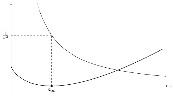
where ⇣(s) ..= P_j ₁j s _{denotes the Riemann-zeta function. This suggests that} the gas cannot achieve densities above a fixed critical density ⇢c( ). Seemingly a paradox, we can explain away this bound by considering separately the density of particles in the lowest energy state. Taking the thermodynamic limit in such a way that hNi/|⇤| = ⇢ > 0, so that h = h⇤ is now a sequence of chemical potentials

chosen to preserve this equality, then for ⇢ > ⇢c( ) we can write ⇢ = ⇢c( ) +⇢0,

where

⇢0= lim

|⇤|!1 1 |⇤|

1

exp( ("0 h)) 1,

which is the density of the ground state. We say that Bose–Einstein condensation (BEC) occurs when⇢0>0, and refer to this as the condensate density.

The derivation above follows the classic approach of Einstein, which is valid for describing the phase transition of an ideal gas. For interacting gasses, however, the energy levels no longer factorise as single-particle energies, and Einstein’s definition no longer has a meaning. A definition of BEC for interacting gases was first provided by Penrose and Onsager [PO56], who studied the 1-particle reduced density matrix. Just as the partition function was defined as the trace of the density matrix ⇤, the

1-particle reduced density matrix is given by the partial trace after integrating out all but one of the particles

˜⇤..=

1

X

n=0

nTrL2

+(⇤n 1) (n)

⇤ . (0.9)

Following [LSSY05], for suitably nice potentialsV at ‘zero’ temperature, i.e. =1, forx, x0₂_R3

˜⇤(x, x0) =N

Z

⇤N 1 0(x, y1, . . . , yN) 0(x

0_{, y}

1, . . . , yN)dy2· · ·dyN, (0.10)

where 0 is the ground state wave function, which minimizes R HN( ). Taking the thermodynamic limit, such thatN/|⇤|!⇢, Penrose and Onsager said that the reduced density matrix has o↵-diagonal long-range order (ODLRO) if the largest eigenvalue of ˜⇤is of the orderNas|⇤|! 1. It can be shown, [PS08] pp.396-7, that

(14)

Moreover, in the case of the ideal gas, this limit agrees with the condensate fraction

lim

|x x0_|!1_|⇤lim|!1˜⇤(x, x 0_{) =}_⇢

0.

The above motivates the common definition that BEC is said to occur in an inter-acting gas, if and only if the 1-particle reduced density matrix exhibits ODLRO. Proving the existence of ODLRO remains a challenge, and has only been achieved in a handful of cases. Notably, [LS02] provides the only rigorous proof of BEC in the continuum for a class of trap potentials, whilst [DLS78, KLS88] prove BEC for a lattice gas at half filling, that is the density of the gas is equal to half the number of lattice sites.

To this point we have described ‘classical’ quantum mechanics: whilst the language of probability is used, at this level we need little probabilistic machinery. This changes in the next section where we provide a probabilistic formula for the partition function of the Bose gas.

Feynman–Kac Formulae

Again we follow the description in [Dan12]. Feynman-Kac formulae were introduced by Feynman [Fey48, Fey53] as a tool to make rigorous his abstract path integral. In the latter of these papers, Feynman derived a formula for the partition function of the Bose gas as an integral over a collection of particle trajectories, where these trajectories are distributed according to interacting Brownian bridges.

Working in the canonical ensemble, Feynman–Kac formulae allow us to derive stochastic representations for kernels of exponential operators. Given the opera-tor exp( tHN), we wish to find a functionKt(x, y) such that

exp⇣ tHN

⌘

f(x) =

Z

⇤NKt(x, y)f(y)dy, f 2L

2 _⇤N _. _(0.11)

To simplify notation we writeH ..₌_H₀₊_V _{in place of} _H_N_{. In the simple case of}

the ideal gas,H=H0= 1₂ and in the infinite volume limit, it is well known that

the kernelKt(x, y) =pt(x, y) satisfying (0.11) is the heat-kernel

pt(x, y).._{= (2}_⇡t₎ d2exp

✓

|x y|2

2t ◆

.

On realising that this is the transition kernel of a d-dimensional Brownian mo-tion, the relationship between Hamiltonian operators and stochastic processes is less mystical. Feynman–Kac type formulae extend for interacting gases,V 6⌘0. A prototypical result is

(15)

and smooth

exp( tH)f(x) =Ex



exp⇣

Z t

0

V(Bs)ds

⌘

f(Bt) , g2L2(Rd). (0.12)

where Ex is the expectation with respect to the Wiener measure Px of a Brownian motion started at x2Rd_,_B

0=x.

A proof is given in [Dan12], whilst an in depth treatment of Feynman–Kac formulae under weaker assumptions is given in [LHB11]. The Feynman–Kac formula for the partition function of a Bose gas is then obtained by applying (0.12) inside the trace (0.4). In the following we letSN denote the symmetric group on [N]..={1, . . . , N}, ie. the set of permutations ⇡: [N] ![N], and write Px,yt [·] = Px[·, Bt = y] for the non-normalised Brownian bridge measure fromx toy over time horizon t >0. Whilst we assumed below (0.3) that the box has periodic boundary conditions, with suitable changes to the definition of Px the following holds for free and Dirichlet boundary conditions as well.

Theorem 0.2(Feynman–Kac Representation of the Bose Gas). LetHN =H0+V,

be the Hamiltonian of a Bose gas where V decays sufficiently fast. The partition function has the representation

Z⇤( , N) =

1

N!

X

⇡2SN

Z

⇤ dx1· · ·

Z

⇤

dxN⇥

N

O

i=1

P_xi,_⇡₍_xi₎

"

exp

✓ _X

1i<jN

Z

0

V(|B_s(i) B(_sj)|)ds

◆#

(0.13) See [Fey53] for the classical reference, or [Gin71] for a rigorous account. Feynman recognised (0.13) as the partition function of a probabilistic model of random per-mutations⇡2SN, whose law we denoteP⇤,N, and conjectured that the occurrence of BEC is signaled by the existence of macroscopic cycles in the random permutation model (i.e. those which grow with the volume|⇤|).

One approach to studying critical phenomena is through the analysis of thermody-namic functions such as the canonical specific free energy or the grand canonical pressure, defined respectively as

f⇢( )..= lim

|⇤|!1 1

|⇤|logZ⇤( , N),

p( , µ).._{= lim}

|⇤|!1 1

(16)

a phase transition. No explicit formula can be derived for the free energy at a fixed particle density and temperature, but from using (0.13) Adams, Collevecchio and K¨onig [ACK11] derive a variational formula for f⇢( ) under general requirements

on the potential V. The variational problem is posed over a space of probability measures which describe marked Poisson point processes on Rd, where the marks are looped trajectories corresponding to the loops over which we integrate in the Feynman–Kac representation. In this description, BEC is recognised via a loss of probability mass in the minimiser of the variational problem, with the interpretation that such a probability distribution puts some mass on infinite cycles.

Feynman’s notion of infinite cycles, or cycle percolation, was made rigorous in a series of papers by Süt˝o [Süt93, Süt02], who took as an order parameter the length

⇠1 of the cycle containing the element 1 2 [N]. Writing P⇤,N for the probability measure on SN induced by (0.13), he showed that in the thermodynamic limit

N/|⇤|!⇢

X

j 1

lim

|⇤|!1P⇤,N[⇠1=j]1,

with strict inequality when⇢>⇢c( ), given in (0.8). The interpretation here is that there is a loss of probability mass, i.e. with non-zero probability the cycle size⇠1 is

infinite. In the second of the two papers this argument is strengthened to say that infinite cycles occur if and only if there is BEC; moreover it is claimed that the proof also holds for the mean-field gas, described by the Hamiltonian HN =H0+ _|_⇤a_|N2

for some constanta >0.

These papers show that in the ideal gas, presence of macroscopic cycles is equivalent to BEC and hence equivalent to ODLRO. However, to make the cycle order param-eter valid for interacting gases a direct relationship to ODLRO must be derived. Letting⇢(n) denote the density of particles belonging to cycles of lengthn,

⇢(n).._{= lim}

|⇤|!1 1 |⇤|nE⇤,N

⇥

#{cyclesc2⇡st. |c|=n}⇤,

Ueltschi [Uel06a, Uel06b] considers the problem of finding a sequence of correlation functionscn(x) and c₁(x) such that

lim

|⇤|!1˜⇤(x, y) =

X

n 1

cn(x y)⇢(n) +c(x y)⇢(1),

where ˜⇤ is the reduced density matrix introduced in (0.10) and one would hope

(at least it is commonly assumed) that⇢(1) =⇢0 is the condensate fraction. This

equality can be shown to hold in finite volume (i.e. before taking the ⇤ limit) for interacting gases, and the coefficientscn,⇤(x y) are given as expectations of single

(17)

fast decaying potentials, Ueltschi demonstrates that this can be carried through to the thermodynamic limit. On the other hand, he provides heuristic arguments suggesting that in a crystalline phase then one can simultaneously have⇢0= 0 and ⇢(1)>0.

Rather than working directly with the permutations which arise from the Feynman– Kac formula, we can work instead with partitions. To a permutation ⇡ 2 SN we associate an integer partition = (⇡), where = ( i)i 1 and i is the number of cycles of lengthiin⇡. We associate to each partition its empirical shape measure, the rescaled Young tableaux Q (k) =N 1P_{j k} j, which describes a probability measure on N. In [Ada08, Dan11] a large deviations analysis is undertaken for the shape measures in the thermodynamic limit|⇤|! 1, and a variational problem is derived. As in [ACK11], BEC is seen through the solution to this variational problem being a sub-probability measure. Whilst the analysis of shape measures forP⇤,N was novel to [Ada08], Vershik [Ver96] had previously performed a similar analysis for the partitions that arise from the momentum space description of the ideal Bose gas, that is the sequences (ni)i 0, wherenidenotes the number of particles in energy state"i. Vershik demonstrates that in the thermodynamic limit the Young tableaux of the typical partition converges to a smooth curve, and identified an exact expression for the limit shape of the ‘mean’ scaled tableaux. A similar analysis is possible in the grand-canonical ensemble, with [Lew86, vdBLP88] considering the mean-field and hard core models from the momentum space description, and [BCMP05] analysing the mean-field model from the loop (Feynman–Kac) perspective.

If we consider instead the box⇤to be a subset ofZd_{, we can derive the lattice} ana-logue of the partition function (0.13), where the probability measuresPx no longer denote Wiener measure, but rather the distribution of a continuous time simple ran-dom walk. T´oth [T´ot93] considers the lattice gas with a discrete approximation to the Lennard–Jones potential, and shows that the grand canonical partition function ⌅⇤( , h) is in fact equivalent to the partition function of the spin-1/2 Heisenberg

ferromagnet. The specific choice of potential allows for a series of manipulations which rewrite the partition function as an expectation with respect to a new ran-dom permutation model: the ranran-dom stirring, or interchange, process. This is a model of a time evolving random permutation, (⇡t)t 0, where ⇡t:⇤ ! ⇤. Each edge in the graph ⇤is equipped with a unit rate Poisson process, and if at time t

the edge (x, y)2⇤‘rings’, then we update⇡t+= (x, y) ⇡t. The partition function

can then be equated to

⌅⇤( , h) =E

2 4Y

n 1

(1 +e hn)l (n)

3 5,

(18)

Bose condensate can be related to macroscopic cycles, but moreover the equivalence to the spin-1/2 model means that infinite cycles also correspond to spontaneous symmetry breaking, and the Mermin–Wagner theorem [MW66]. A detailed survey of the random stirring process is the content of [Dan12].

In the next section we describe the Markov loop soup: a Poisson point process on a space of lattice loops, which will be the starting point for our own analysis of the Bose gas. We have already mentioned that [ACK11] considered the Bose gas as a marked Poisson point process onRd_{, where the marks are Brownian loops. A point process} approach was also taken by Rafler [Raf09], for the ideal gas in Rd. Rafler studies the Martin–Dynkin boundary of the point process: heuristically, the collection of all other point processes which locally resemble the one of interest. In the grand canonical ensemble, it is shown that this set contains only a single process, and says there is no phase transition. In the canonical and microcanonical ensembles, Rafler proves that the Martin–Dynkin boundary is a convex (non-singleton) set of mixed Poisson processes, and says a phase transition occurs. Rafler also considers geometric aspects of the ‘typical’ loop: such as the location of the barrycentre, and percolation questions. In some respects this has the closest similarity to our own work, where we will study the geometry of the Poisson point process via its associated occupation field, and relate the thermodynamic functions of the grand canonical Bose gas with correlations in this field.

II

A Survey of Markov Loop Soups

Just as the probabilistic models described above have a physical derivation, the Markov loop soup also owes its conception to the physics community, where it arises via a functional integral description of a lattice model.

In [Sym66, Sym69], Symanzik provided a heuristic description of '4-quantum field theory in terms of a gas of interacting Brownian loops. On considering lattice field theories in place of Symanzik’s continuum model, Brydges, Fr¨ohlich and Spencer [BFS82] were able to make rigorous the connection between the two models. A concise version of this equivalence can be described for the Gaussian case.

Let P be the transition matrix of a symmetric random walk, X = (Xt)t 0, on a

lattice box⇤⇢Zd_,_d _{1, and consider the Gaussian field described by}

PG_(d_'_{) =}_Z 1

⇤ e h',(I P)'id',

(19)

random walk

Cov('x,'y) = (I P)xy1 = Ex

Z ₁

0

1

_{Xt=y}dt =..Gxy, (0.15)

which is immediate fromGxy =P_n ₁Pxyn, Corollary 1.5. Symanzik’s formula pro-vides a deeper understanding of the link between Gaussian fields and random walks, notably relating the partition functionZ⇤of the Gaussian field to a sum over families

of random loops.

Theorem 0.3 (Symanzik’s Formula). The partition functionZ⇤ of the lawPG can

be expressed as

Z⇤=

X

n 0

1

n!

X

x2⇤

Z ₁

0

1

tPx[Xt=x]dt

!n

(0.16)

See [BFS82]. This formula holds in the greater generality of the partition function of a'4-theory, and we return to this in Section 3.3.1 where we discuss an interpretation for the Bose gas. Inspired by the work of Symanzik and Brydges et al., Dynkin [Dyn83] provided an extension of (0.15) for correlations for the square of a Gaussian field. Defining the local time at ‘infinite time’ of a random walk X = (Xt)t 0 to

be the random variable lx = R₀1

1

_{Xs=x}dt, then under the measure Pxy[·] =

R₁

0 Px[·, Xt=y], Dynkin’s theorem says.

Theorem 0.4 (Dynkin’s Isomorphism). For any bounded measurableF:R⇤!R

Exy⌦EG 

F ✓

lx+1

2'

2

x

◆

=EG 

'x'yF

✓

1 2'

2

x

◆ .

See [Szn12], pp.35-6. An extension to complex Gaussian measures was given by Brydges, [Bry92]. Symanzik’s work for Euclidean quantum fields, and Feynman’s description of the Bose gas are both examples of the functional integral approach to statistical mechanics. Other important examples are Aizenman’s random walk description of the Ising model [Aiz82], and the more recent work of Brydges and Slade (along with an ensemble of collaborators) regarding the functional integral description of the self avoiding random walk, for a survey see [BIS09].

Independently of the relevance to statistical mechanics, ensembles of loops have been the focus of recent work in probability. Letting tdenote the collection of continuous time loops on a graph ⇤: i.e. c`adl`ag paths : [0, t]!⇤ with (0) = (t), Le Jan defined a measureµ⇤on the space =[t>0 t by

µ⇤(G)..=

X

x2⇤

Z ₁

0

1

tPx[G, Xt=x]dt, (0.17)

(20)

comprehensive analysis of theMarkov loop soup: the family (P↵)↵>0of Poisson point

processes on the set described by the intensity measures ↵µ⇤. A configuration S⇢ (where we abuse notation and write ‘⇢’ althoughSmay in fact be a multiset under the law P↵) defines a random fieldL= (Lx)x2⇤ called the occupation field,

where

Lx=Lx(S)..₌X

2S

Z _{| |}

0

1

_{ (s)=x}ds, x2S,

with| | the length of the loop (i.e. the uniquet >0 for which 2 t). Amongst many results regarding the properties of L, Le Jan provides an interpretation to Symanzik’s formula and Dynkin’s isomorphism via the loop soup.

Theorem 0.5 (Le Jan’s Isomorphism). Let G = (Gxy)x,y2⇤ be the Green’s

func-tion associated with the random walk P, and PG _{the law of the associated centred} Gaussian field. Then

⇣

(1 2'

2

x)x2⇤, PG

⌘ _(d)

= ⇣(Lx)_x2⇤, P↵=1 2 ⌘

.

That is, the occupation field of the Markov loop soup at intensity ↵= 1₂ is equal in distribution and the square of a Gaussian field.

See [Szn12], pp.90–1. Whilst the essence of this theorem was already present in the work of Symanzik and Brydges et al., their work does not recognise the right hand side of (0.16) as the normalising constant of a Poisson point process.

It would be amiss at this point not to mention that prior Le Jan’s work, Lawler and Werner had already sparked interest in loop soups. In [LW04] they consider the loop measure3_{(0.17) but with}_Px _{now the distribution of a Brownian motion in}_C_,

which they relate to the Schramm–Leowner evolution (SLE) processes. Later papers of Sheffield and Werner [SW12] and Qian and Werner [QW15] relate the Brownian loop soup to the conformal loop ensembles (CLE), a non-Poissonian collection of mutually and self avoiding random loops in C: these arise as the outer boundaries of clusters in the Brownian loop soup.

Another variant on the loop soup is to consider the discrete time random walk loop soup. An n-loop is a finite sequence z = (z(i))n_i₌₀ withz(i)2⇤, and z(0) =z(n). A discrete loop measure, µD_{, is defined on the collection of all discrete loops in} _⇤ via

µD(z)..₌ 1

nPz(0)z(1)· · ·Pz(n 1)z(n)Pz(n)z(0), 3

(21)

with P a symmetric transition matrix on ⇤; basic properties of this measure are outlined in [LL10]. Lawler and Trujillo Ferreras [LTF07] proved that the Brownian loop soup can be derived as the scaling limit of a discrete time random walk loop soup onZ2_{, whilst Lawler and Perlman [LP14] define the occupation field of discrete}

loops, from which they derive an alternative proof of Theorem 0.5. This proof is adapted in [Cam15] to provide an isomorphism theorem between a Gaussian free field (not the square of the field!) and the loop occupation field where the sign of the occupation fieldLx is changed according to an Ising type interaction.

Another random field associated with the discrete (and for that matter the contin-uous) loop soup is the covering fieldC= (Ce)e2⇤2{0,1}⇤, which is now indexed by

the edges of the graph. For a configuration of discrete loopsS we set

Ce=

8 < :

1 if9z2S st. e2z, 0 else.

That is, the edge e is open, Ce = 1, if and only if there is a loop which crosses it. When ⇤ = Zd, d 1, as for Bernoulli bond percolation, we can define the probability ✓(↵) that under the measure P↵ the cluster of Ce which contains the

origin has infinitely many edges. Le Jan and Lemaire [LeJL13] prove that ✓ is increasing in ↵ > 0, and via a simple coupling with bond percolation provide a lower bound on the critical intensity ↵c ..= inf{↵ > 0 : ✓(↵) > 0}. Chang and Sapozhnikov [CS14] proved that for d = 1,2, ↵c = 0, whilst for d 3 the phase transition is non-trivial: ↵c > 0, and using a coupling to the Gaussian free field Lupu [Lup14] proved that in fact↵c> 12.

III

Summary of Contents and Structure

In the preceding sections we saw how models for random loops have arisen in two distinct contexts: the probabilistic analysis of the Bose gas, and the study of Gaus-sian fields and isomorphism theorems. Introducing a Bosonic loop measure, our analysis aims to concurrently develop the literature of the Bose gas, and loop soups. We approach these topics from two directions:

How do functionals of the Bosonic occupation field relate to the thermody-namic properties of the ideal gas? Moreover, can we characterise BEC in terms of behaviour of the occupation field?

To what extent can we carry through the analysis of the occupation field under

µ⇤to the Bosonic loop measure? In particular, does the Bosonic loop measure

(22)

The loop measure we consider is given by

µB

,h,⇤(G)..=

X

j 1

X

x2⇤

e hj

j P

j xx[G].

This di↵ers from the measureµ in two aspects. The most immediate di↵erence is that rather than allowing loops of all durations t > 0, we restrict to those loops whose duration is exactly an integer multiple of > 0. The second distinction is the addition of the term e hj_{, and we will look to study the behaviour of the loop} model as we vary h0. This is in contrast to Le Jan, who considers varying the intensity with the factor↵which is independent of the loop lengths.

Letting =[j 1 j denote the space of all loops, we will see that

exp µB

,h,⇤( ) =⌅⇤( , h),

where⌅is now the grand canonical partition function of an ideal lattice Bose gas. In-terpreting the partition function on the right hand side as the normalisation constant of a probability measure, we recognise this as none other than the normalisation of a Poisson variable with intensityµB

,h,⇤( ). Moreover, lettingS denote the Poisson

point process induced byµB

,h,⇤, we have

P

2 4X

2S

| |= N 3 5= e

hN_Z

⇤( , N)

⌅⇤( , h) ,

which should be compared to (0.5). The above formulae, which we prove in Sec-tion 1.2 and SecSec-tion 2.2 respectively, give the interpretaSec-tion of the loop soup as a poissonization of the canonical ensembles of the Bose gas, which is exactly to say that it describes the grand canonical ensemble.

Thesis Outline

In Chapter 1 we formally introduce the Bosonic loop measure, and its related loop soup and occupation field. In this section we also clarify our definition of graphs and their spectra, and detail the sense in which we will consider thermodynamic limits in this thesis.

We start our analysis of the Bosonic occupation field in Chapter 2 where we consider the mean occupation on the graph, and prove that in the limit this converges to a degenerate distribution. In turn this is related to the density of the ideal Bose gas, and we provide a definition for BEC of an ideal Bose gas on a graph.

(23)

this does not agree with that of a Gaussian process. Introducing a di↵erent space-time loop measure we show that this measure does have a description in terms of complex Gaussian fields. Further we see that the space-time occupation field provides an interpretation to the 1-particle reduced density matrix of the ideal gas. Having established several results for the ideal gas, in Chapter 4 we consider possible Hamiltonians defined on the occupation field, in particular focusing on two mean-field models. We present a large deviations analysis for the mean-mean-field models, focused on deriving expressions for the critical density.

Finally, Chapter 5 gives an overview of further topics for consideration, and provide some closing remarks.

(24)

Chapter 1

Definitions and Preliminary

Results

We commence by introducing some basic terminology and definitions. In the first section we describe graphs and their associated Markov processes, we introduce the local time and Green’s function of a process, and define the sense in which we will take thermodynamic limits of graphs. In the second section, we define formally both the Markov and Bosonic loop measures, their associated Poisson processes, and occupation fields.

1.1 Random Walks on Graphs, and Their Limits

Throughout this thesis when we refer to a graph we will mean not only the graph structure (i.e. edge and vertex sets), but also to a random walk defined on the structure. As a consequence, we define a graph to be a triple (⇤, w,), with ⇤ a finite set, w:⇤⇥⇤ ! R+ a weight function, and : ⇤ ! R+ thekilling vector,

where we useR+ to denote the positive reals. The set⇤corresponds to the vertices

of the graph, whilst for pairsx, y 2⇤ withwxy ..=w(x, y)> 0, we say there is an edge fromxtoy. The weights themselves, together with the vector, determine a family of Markov processes, as described in the coming section. To simplify notation, henceforth we will simply write ⇤to denote the triple⇤= (⇤, w,).

1.1.1 Weighted Graphs and Their Markov Generators

A graph induces a family of Markov processes whose jump distributions are de-termined by the functions w,. To facilitate the definition we enlarge the vertex set to ⇤⇤ = ⇤[{Ü}, where the additional vertex Ü is called the cemetery state. The discrete time Markov chain (Z⇤

(25)

P⇤= (Pxy⇤)x,y2⇤⇤ defined forx, y6=Üto be

Pxy⇤ =

wxy

x , P ⇤ xÜ= x

x, P ⇤

Üy= 0, PÜÜ⇤ = 1,

where x..=x+Py2⇤wxyforx6=Ü, and we set Ü= 0. We refer to : ⇤!R+as

therate vector. In turn, P⇤ is used to define a continuous time Markov process on ⇤⇤with unit exponential jump rates. Denoted (X_t⇤)t 0, the process is determined

by its generator (P⇤ _I_{), with} _I _the _|_⇤⇤_|_⇥_|_⇤⇤_| _{identity matrix. We also define} (X⇤t)t 0 with variable exponential jump rates, which leaves site x2⇤⇤ at rate x:

it is determined by the generatorQ⇤= (P⇤ I). In the case that6⌘0, all three processes above will almost surely visit the siteÜ, after which we say that they are killed.

We work throughout with the induced sub-stochastic processes on ⇤, and refer to these asrandom walks. We define the law and expectation of the processesZ, X,X

conditioned to start fromx2⇤byPx,Ex, and writingP, Qfor the cofactors ofP⇤

andQ⇤_{obtained by deleting the row and column corresponding to}_Ü_{, we have}

Px⇥Zn=y

⇤

= Pn _xy, Px⇥Xt=y

⇤

= et(P I) _xy, Px⇥Xt=y

⇤

= etQ _xy.

We stress that these are not true probability measures, in that if  6⌘ 0, then summing overy2⇤the expressions may total less than 1. We briefly describe the standard coupling of the walks X,Xto Z. Given a path Z = (Zn)n 1 distributed

according toPx, defineJ0= 0, andJn⇠Exp(1) i.i.d. exponential variables,n 1. Then the path

Yt=Zn, forJntJn+1

is equal in distribution to X under Px. If instead I0 = 0 and In ⇠ Exp( Zn) are independent and exponentially distributed according to the rate of the current state, the resulting pathYthas the distribution ofXunderPx. Throughout we will assume that graphs are loop free, wxx = 0 for all x 2 ⇤, and irreducible: for all

x, y2⇤there is ann 0 such thatPn xy>0.

1.1.2 Random Walk Local Time and the Green’s Function

Forx2⇤we define thelocal time atxof the walkXto be the random variable

lT_x⇣X⌘..₌

Z T

0

(26)

We define the local time ofX similarly, and replacing the integral with a sum, the local time of Z. Similarly we define the local time ‘at infinity’ by

lx

⇣

X⌘=

Z ₁

0

1

_{_Xs₌_x_}ds,

where as before we can interchangeX for either ofX or Z; this variable exists as an extended real number, and satisfies.

Proposition 1.1. Suppose  6⌘ 0, then for x, y 2 ⇤, ly is Px-a.s. finite, and Ex[ly]<1. Conversely, if ⌘0, then Px-a.s. ly=1.

Proof. The proof is classical, and for brevity we prove it only in the casewxy,x>0 for allx, y2⇤; see [LPW09] Lemma 1.13 pp.11-2 for a more detailed proof (though not in the context of local times). In light of the standard coupling it suffices to prove the proposition only in the case of the discrete walk Z, so thatly= #{n 0 : Zn= y}. Moreover, we couple Z with the walkZ⇤ on the space ⇤[{Ü}, and definingT = inf{n 0 : Zn⇤=Ü}, then

Ex

2 4X

y2⇤

ly

3

5=Ex[T 1].

Let".._{= infy}_P⇤

yÜ>0, which is strictly positive due to our assumptionx>0 for all

x2⇤. In particular, for allk 0, Px[Zk+16=Ü|Zk6=Ü](1 "). Then

Ex[T] =X n 0

Px[T > n]

=X n 0

Px[Z₁⇤, . . . , Z_n⇤6=Ü]

X

n 0

(1 ")n

=" 1

HenceEx[ly]PyE[ly]" 1<1.

In the case  ⌘ 0, let Ty ..= inf{n 0 :Zn = y}, then the same proof as above asserts thatEx[Ty]<1, and in particularPx[Ty<1] = 1. Consequently, not only does Znalmost surely visit y, it visits infinitely often, and hence Ex[ly] =1. Henceforth we say that the graph⇤is recurrent if⌘0, else we say it is transient. The Green’s function associated to a walkX is the matrix of expected local times at infinity

Gxy X ..=Ex

h

ly

⇣

(27)

which exists as an extended real number. DefiningGxy(X), Gxy(Z) analogously, if the graph is recurrent then

Gxy X =Gxy X =Gxy Z =1.

The following proposition allows us to extend this equality to the transient case. In the following we use (d)= to denote equality in distribution.

Proposition 1.2. For x, y2⇤, under the lawPx

ly

⇣

X⌘ (d)= _y1ly(X).

Proof. It suffices to show that the two variables have the same cumulative distribu-tion funcdistribu-tion: PxhlTy

⇣

X⌘ti=Px⇥ 1lTy(X)t

⇤

,t2R. Let N (respectivelyN) denote the total number of visits thatX (resp. X) makes toyin timeT. From the standard couplingN (d)= N, so

PxhlTy(X)t

i

= 1

X

n=0

PxhlTy(X)t N =n

i

PxhN=ni

= 1

X

n=0

PxhlTy(X)t N =n

i

Px⇥N=n⇤,

so it suffices to show: Px⇥lT

y X t N=n

⇤

=Px⇥ 1

y lyT(X)t N =n

⇤

,n 0. But this follows since on the eventN=N =n, the coupling gives

lT_y⇣X⌘ =

n

X

k=1

Ik = y1

n

X

k=1

Jk = y1lTy(X),

whereIk⇠Exp( y) andJk⇠Exp(1) are all i.i.d. and we used the scaling relation for exponential variables: Exp( y) = 1

y Exp(1).

Since equality in distribution implies that the expectations agree, it follows that

Gxy X = y1Gxy X <1. (1.2)

Moreover, sinceE[Exp(1)] = 1, then

Gxy(X) =Gxy(Z).

1.1.3 Graph Spectra and Spectral Convergence

In this section we provide several basic facts about the spectra of the matrices

(28)

Chapter 2. For a square matrix,A, we denote Spec(A) for its spectrum, i.e. the set of eigenvalues ofA.

Theorem 1.3. The spectrum ofP satisfies

Spec(P)⇢{z2C: |z|1}.

Furthermore,Spec(P)⇢{z2C: |z|<1}if and only if 6⌘0.

Proof. Since⇤is irreducible,P satisfies the conditions of the Perron–Frobenius the-orem, [HJ13] p.534. Defining thespectral radius to be⇢= max{|⌘|:⌘2Spec(P)}, there is a positive vectorvx 0 for which⇢is a corresponding eigenvalue: P v=⇢v, and

0min x

X

y

Pxy⇢max

x

X

y

Pxy1.

If⌘0, thenP_yPxy= 1 for allx2⇤, and so 1 is an eigenvalue, and⇢= 1. Now suppose  6⌘ 0, and that there is a positive vector v such that P v = v; in particular since⇤ is loop free we havevx = Py=6 xPxyvy, for any x2⇤. Choosing

z such thatvz is maximal

vz=

X

y6=z

Pzyvyvz

X

y6=z

Pzy vz,

which is a contradiction unless both inequalities are in fact equalities. But since v

is positive,P_y₆₌_zPzyvy=vzPy6=zPzy holds only ifv is a constant,v⌘c >0. But then for anyx2⇤

c=vx=c

X

y

Pxy,

so thatP is stochastic, which contradicts6⌘0. We say that a random walk isreversible if it satisfies

xPxy= yPyx, x, y2⇤.

Corollary 1.4. IfP is reversible, then the eigenvalues ofP are real, andSpec(P)⇢ [ 1,1]. If in addition 6⌘0, thenSpec(P)⇢( 1,1).

Proof. In light of the previous theorem it suffices to prove thatP has real eigenval-ues. Defining the inner-product

hu, vi ..=X x

(29)

we note thatP is self-adjoint for this inner product

hu, P vi =X

x xux

X

y

Pxyvy

!

=X y

y

X

x

Pyxux

!

vy=hP u, vi .

It follows immediately thatP has real eigenvalues.

As a consequence we also obtain the following representation of the Green’s function of the random walk.

Corollary 1.5. If 6⌘0, then the Green’s function is given by

G X =G Z = (I P) 1.

Proof. Working with the discrete walk we note

Gxy = E

"₁ X

n=0

1

_{Zn=y}

#

= 1

X

n=0

P[Zn=y] = 1

X

n=0

P_xyn.

From Theorem 1.3 the spectral radius ofP is strictly less than 1, and so the matrix power series above converges to (I P) 1_{by Proposition B.20.}

Turning to the generator of a continuous time process, we observe that it is no longer possible to find a uniform bound on the spectrum. We denote H ..₌ _{_z ₂

C: Re(z)0}.

Theorem 1.6. Let ⇤= maxx₂⇤ x. The spectrum ofQsatisfies

Spec(Q)⇢{z2C: |z+ ⇤|| ⇤|}⇢H.

Further, if 6⌘0thenQis non-singular, andRe(⌘)<0, for all ⌘2Spec(Q). Proof. The first part is an application of the Gerˇsgorin circle theorem, which gives that

Spec(Q)⇢ [ x2⇤

n

z2C: |z+ x| xPy2⇤Pxy

o ,

see [HJ13] pp.388-9. SinceP is (sub)-stochastic,P_yPxy1, and

⇢ [

x2⇤

{z2C: |z+ x|| x|},

which in turn is a subset of the largest disc centred at ⇤.

(30)

x 2⇤ such that |Qxx| > P_y₂_⇤_\{_x_}|Qxy|. We have already assumed thatP (and henceQ) is irreducible, and choosingx2⇤such thatx6= 0

Qxx= x> x

X

y2⇤\{x}

Pxy =

X

y2⇤\{x}

Qxy.

As we will see in Chapter 2, several statistics of loop occupation fields are determined entirely by the spectrum of the graph. Consequently in taking graph limits it will often suffice only to study the limit of the spectra; in the following we provide the notion of convergence which will be used in later chapters.

Definition 1.7. The (empirical) spectral measure of a finite graph ⇤ is defined as the measure m⇤ onH equipped with the Borel -algebra

m⇤(dx)..= 1

|⇤|

X

⌘

⌘(dx),

where the sum runs over the eigenvalues⌘2Spec(Q), and a denotes the Dirac (or degenerate) distribution with atom at a2R.

Note that integration against the spectral measure is no more than a summation

Z

Hf(x)m⇤(dx) = 1 |⇤|

X

⌘

Z

Hf(x) ⌘(x)dx= 1 |⇤|

X

⌘

f(⌘). (1.3)

A sequence of probability measures (mn)n 1onCis said to convergein distribution

(orweakly) to a measurem₁ if given any bounded continuous functionf:C!R

lim n!1

Z

f(x)mn(dx) =

Z

f(x)m1(dx).

In this case, we writemn

(d)

!m₁. Noting that f(x)⌘1 is a bounded continuous function on C, then

m₁(C) =

Z

C1m1(du) = limn!1

Z

C1mn(du) = 1

so that any weak limit of a sequence of probability measures is itself a probability measure. Our notion of graph convergence will be through convergence in distribu-tion of the associated spectral measures.

Definition 1.8. Let ⇤n = (⇤n, wn,n)1n=1 be a sequence of graphs, and write mn=m⇤n for the spectral measures. We say that the sequence (⇤n)n 1 is a (spec-trally) convergent graph sequence if there exists a measurem₁ to which the spectral measures converge in distribution,mn

(d) !m₁.

(31)

Given a bounded Lebesgue measurable domain D ⇢ Rd _{with Lebesgue measure} |D|= 1, we say that a measurable function ⇤:D!His a distribution for⇤ifm⇤

is obtained as the pushforward measure of Lebesuge measure under ⇤

m⇤(B) = ⇤1(B), B✓H measurable.

We recall that the change of variables formula for pushforward measures allows us to write integrals against m⇤as

Z

Hf(y)m⇤(dy) =

Z

D

f ⇤ (x)dx, (1.4)

where f: H ! R is measurable, and the integral on the right hand side is with respect to Lebesgue measure. The following proposition enables us to confirm con-vergence of the spectral measures by studying associated distribution functions. Proposition 1.9. Let (⇤n) be a graph sequence, and n: D ! H a sequence of distribution functions on the same domainD⇢Rd_{. If there exists}

1:D!Hsuch that n ! 1 pointwise almost everywhere, then the graph sequence ⇤n converges, and the limit measure m₁ is given by the pushforward of ₁

m₁(B)..₌_| 1

1(B)|, B✓H measurable.

Proof. Almost everywhere pointwise convergence of the sequence ( n)n 1 implies

that for any continuous boundedf:H!Rthe compositionf n!f 1 almost everywhere. Boundedness of f ensures that f n is uniformly bounded, that is there is an M such that (f n)(x)  M for all x 2 D and n 1. Moreover, boundedness of the domainDensures

Z

D

(f n)(x)dxM Z

D

1dx=M|D|,

from which the claim follows via the dominated convergence theorem.

For a graph⇤with spectrum Spec(Q) = (⌘j)|_j⇤₌₁| , the simplest choice of distribution function is ⇤: (0,1]!H defined to be

⇤(u) =⌘d|⇤|ue.

We refer to this as thecanonical distribution function, and for most cases it suffices to study only this function. The greater generality in which we defined distribution functions will however be useful when proving convergence for lattice boxes⇤⇢Zd_,

(32)

Complete Graph

ForN 2, we define the complete graph onN vertices byKN = ([N], w,), where for allx, y2[N]

wxy=x= 1

N.

Subsequently the continuous time walkXis the simple random walk with unit jump rate and which is killed according to a geometric random variable with mean N. The eigenvalues ofQare

⌘1=· · ·=⌘N 1= (1 + 1

N),⌘N =

1

N.

The sequence (KN)N 2is spectrally convergent, and has limit measurem1 = 1.

Lattice Boxes

ForN 1 define the lattice box⇤N = [ N, N]d\Zd_{, for} _d _{1. We will consider} two di↵erent random walks on⇤N. The first is defined by the weight function

w(dir)

xy =

8 < :

1

2d if|x y|= 1, 0 else.

and killing vector(dir)

x = 1 Py2⇤Nwxy. This definesX, the continuous time simple random walk killed on exiting the box⇤N. We say that ⇤(dir)

N = (⇤N, w(dir),(dir)) is the lattice box withDirichlet boundary conditions. Alternatively we can define the weighting

w(per)

xy =

8 < :

1

2d if91idst. xi= yi=±N, andxj=yj, j6=i, 0 else.

with (per) _⌘ _{0, for which}_X _{is the continuous time simple random walk on the} _d

-torus, and we call⇤(per)

N = (⇤N, w(per),(per)) the lattice box withperiodic boundary conditions. In the case of ⇤(per)

N , the spectrum is

Spec(Q(per)

) =

(

1

d

X

i=1

cos

✓

2⇡ ji

2N+ 1

◆

1 : j= (ji)di=12{1, . . . ,2N+ 1}d

(33)

The sequence⇤(_Nper)converges in distribution, and the limit measure m1 is defined via its distribution function ₁: [0,1)d![ 2,0]

(per)

1 (u) = 1

d

X

i=1

cos(2⇡ui) 1.

Rather than defining the spectrum of⇤(dir)

N directly, a comparison argument yields convergence of the sequence⇤(dir)

N , and

(dir)

1 = (1per).

1.2 Loop Measures, Soups, and Their Occupation Fields

Givent >0, a c`adl`ag functionp: [0, t]!⇤with finitely many points of discontinuity

0 = t0 < t1 < · · · < tn < t is said to be a path on ⇤ if the sequence of vertices

xj=p(tj) are such thatw(xj, xj+1)>0 forj = 0, . . . n 1. Let Dt denote the set of all paths of duration t, and D =[t>0Dt the set of all paths. Given p 2D, we denote|p|for its duration: the uniquet such thatp2Dt. A path whose start and end points agree is called aloop, we denote

t..={ 2Dt: (0) = (t)}

for the set of length t > 0 loops, and = [t>0 t for the set of all loops. A path with no discontinuities is by default a loop, and we call this apoint loop.

Following [Szn12] pp.35-6, we construct a -algebra onD(respectively, ) as follows. We define a bijection : D ! D1⇥(0,1), where p 7! (˜p, t) with t = |p|, and

˜

p(s) =p(st). We endowD1⇥(0,1) with the product -algebra A⇥B, whereB

is the Borel -algebra on (0,1), and A is the -algebra generated by the family of sets As,x = {p 2D1:p(s) = x}, with s 2[0,1], x 2⇤. We observe thatA is a

natural choice as it is none other than the Borel -algebra induced by the Skorokhod topology onD1, see [Bil99] pp.134–5. Finally, using the projection we define

D= 1(B) : B2A⇥B ,

which is a -algebra onD. In the same way we defineG, a -algebra on .

1.2.1 The Measures

µ

and

µ

B

As before, let P denote the law of a random walk on ⇤. For t > 0, we define a measure on paths from xtoy by

(34)

We call this the (normalised) random walk bridge measure, where the term non-normalised stems from the fact that this is not a probability measure: Ptxy[D] = Px⇥Xt=y⇤1. We define two families of measures on , theMarkovloop measures

µh,⇤(G)..=

X

x2⇤

Z ₁

0

eht

t P

t

xx[G]dt, G2G. (1.5)

and theBosonic loop measures

µB

,h,⇤(G)..=

X

x2⇤

X

j 1

e hj

j P

j

xx[G], G2G. (1.6)

The parameter h <0 is called the chemical potential, whilst > 0 is theinverse temperature. We note thatµh,⇤depends only onh, since adding the relevant terms

in > 0 act only as a change of variables in the definition. Henceforth we freely denoteµ, µB _{for the Markov and Bosonic loop measures respectively, including the} various subscripts only when we wish to highlight the dependence on the graph structure, or values of andh. We remark that in the case h= 0, the measure

µ0 is exactly the loop measure studied by Le Jan [LeJ10, LeJ11], and many of the

properties which he studies can be generalised forµh, h <0: one of these will be the isomorphism theorem, which we discuss in Chapter 3.

We briefly comment that our convention di↵ers from that used elsewhere in the literature. As remarked in the introduction, in particular the footnote on page xviii, for most authors a loop is defined as a conjugacy class of /⇠ where ⇠ is the equivalence relation which equates all loops which can be obtained from one another by a time shift (i.e. by forgetting their root); the loop measure µh is constant on conjugacy classes, and so determines a measure on the space /⇠. Since the random variables we consider will not be e↵ected by whether or not our loops are rooted, we will not make use of this equivalence relation, and keep the convention that a loop is endowed with its root, (0).

Lemma 1.10. Assume6⌘0. Fix >0, h0, then (i) µis a -finite measure.

(ii) µB _{is finite with}

µB_{( ) =} _Tr⇣_log⇣_I _e (Q+hI)⌘⌘_<₁_.

If ⌘0, then the above hold if and only if h <0.

Proof. For a proof that µ0 is -finite, see [Szn12], p.63; from the definition, for

(35)

For (ii), we have

µB( ) =X x2⇤

X

j 1

e hj

j Px

h

X j=x

i

=X x2⇤

X

j 1

e hj

j ⇣

e jQ⌘

xx

=X x2⇤

X

j 1

1

j ⇣

e (Q+hI)⌘j

xx.

Appealing to Proposition B.22, the series overj 1 converges if the spectral radius of exp( (Q+hI)) is less than 1. Letting Spec(Q) ={⌘j}|j⇤=1| , we require

max j |e

(⌘j+h)_|_{= max} j e

(Re(⌘j)+h)_<₁_,

where Re denotes the real part of a complex number, and we relied on the fact that forz 2C, |exp(z)|= exp(Re(z)). But from Theorem 1.6, Re(⌘j)0 holds for all

j = 1, . . . ,|⇤|, and so the inequality above holds whenever h < 0. On the other

hand, if6⌘0, then the same theorem for the spectrum asserts that Re(⌘j)<0, so that the inequality holds forh= 0.

On recalling that Tr(log(I A)) = log det(I A), justified below Proposition B.22, the formula above gives

exp µB_{( ) =} |⇤|

Y

j=1

⇣

1 e (⌘j+h)⌘ 1_,

where as above we denote ⌘j for the eigenvalues of Q. On comparing this with (0.7) we see that this is none other than Einstein’s formula for the grand canonical partition function of the ideal gas. In the following we give a direct argument of this fact, which does not rely on the spectral representation.

Theorem 1.11. For any >0and h <0

exp µB

( ) =⌅⇤( , h).

Proof. To simplify notation in the following we writez= exp( h), which is known as thefugacity, and writePj=P_x₂_⇤Px⇥X j=x⇤, given these notational simplifica-tions, the total mass of the loop measure becomesµB_{( ) =} P

j 1z

j

jPj. Expanding the exponential power series

exp µB_{( ) =} X m 0

1

m!

0 @X

j 1

zj

j P

j

1 A

m

(36)

each power inmcan further be expanded using the multinomial theorem for power series = X m 0 1 m! X

P_kj₌_m

✓ m k ◆ Y j 1 ✓

zj_Pj

j ◆kj

,

where the sum is over sequencesk= (kj)j 1withPjkj=m, and m_k =m!/Qjkj! is the infinite multinomial coefficient. Canceling the factorial terms, we see that the sum depends onmonly through the sequencesk, so we write

= X P_kj< 1 Y j 1 1

kj!

✓

zj_Pj

j ◆kj

,

where the sum now runs over all terminating sequencesk= (kj)j 1. We factor this

as a summation over integer partitions: i.e. fixing n 0, consider those sequences

ksuch thatP_jjkj=nwith the interpretation that there arekj blocks of lengthj. Now

=X n 0

X

P

jkj=n

Y

j 1

1

kj!

✓

zjPj

j ◆kj =X n 0 1 n! X P

jkj=n

Y

j 1

n!

kj!jkjz

jkj_Pkj j .

Recognising the combinatorial factor n!/(kj!jkj) as the number of permutations

⇡ 2Sn with exactly kj cycles of length j, we can instead sum over permutations. Denotingcfor a cycle in a permutation⇡, andnc for the length of the cycle

=X n 0 1 n! X ⇡2Sn Y c2⇡

zncPnc

=X n 0

zn

n!

X

⇡2Sn

Y

c2⇡

Pnc. (1.7)

Working in the opposite direction, we note that for a permutation ⇡ 2 Sn with cycles c= (c(1), . . . , c(nc))

X

x1,...,xn2⇤

n

Y

i=1

PxihX =x⇡(i)

i

= X

x1,...,xn2⇤ Y

c2⇡

nc

Y

i=1

Pxc(i) h

X =xc(i+1)

i

, (1.8)

with the conventionc(nc+1) =c(1). The second sum depends only onxc(1), . . . , xc(nc)

and so we can factorise the sum as

=Y c2⇡

X

x1,...,xnc

nc

Y

i=1

Px_c₍_i₎hX =xc(i+1)

(37)

and the Chapman–Kolmogorov equation gives

=Y c2⇡

X

x

PxhX nc=x

i

=Y c2⇡

Pnc.

Substituting (1.8) into (1.7) we obtain

exp(µB_{( )) =}X n 0

zn

n!

X

⇡2Sn

X

x1,...,xn2⇤

n

Y

i=1

PxihX =x⇡(i)

i

=X n 0

znZ⇤( , n),

whereZ⇤( , n) is recognised as the graph analogue of the canonical partition

func-tion (0.13), and the result follows from (0.5).

1.2.2 The Poisson Loop Soup

We start by providing a formal definition of the Poisson point process for loop measures as a random measure, for which we follow [Kal01] pp.225-6, after which we give a more user friendly description.

A counting measure on ( ,G) is a measure taking integer values, ⇠:G ! N, and we denote N ..₌ _N₍ _,_{G) for the set of all} _{-finite counting measures on (} _,_G).

For G2 G, we define the evaluation map ⇡G: N ! N by⇡G(⇠) = ⇠(G), and let F ..= (⇡G: G2G) be the smallest -algebra for which the evaluation maps are measurable. Thus, we have defined a measure space (N,F) of counting measures. A point process is any probability measurePon (N,F). Given a measurable function

F:N !R, we denote the expectation with respect toPby

E[F]..=

Z

N

F(⇠)P[d⇠].

We consider point processes as the law of a random measure⇠: that is, rather than considering events{⇡_G1(C)}, we write the equivalent {⇠(G)2C}. We state with-out proof the following uniqueness criteria for point processes [Kal01], Lemma 12.1 pp.225-6.

Lemma 1.12. A point process is uniquely determined by its finite dimensional dis-tributions. That is the point processes ⇠ with law P, and⌘ with lawePare equal in distribution, ⇠ (d)= ⌘ if and only if for all n 1,G1, . . . , Gn2G

⇠(G1), . . . ,⇠(Gn)

(d)

= ⌘(G1), . . . ,⌘(Gn) .

(38)

⌫ is the lawPon (N,F) with the defining properties Poisson property. ForG2G andn 0

P[⇠(G) =n] =e ⌫(G)⌫(G)

n

n! .

Independent increments. For pairwise disjoing sets G1, . . . , Gk 2 G, the variables⇠(G1), . . .⇠(Gk) are pairwise independent underP.

Any ⇠ 2 N can be associated with a countable (or finite, if ⇠ is finite) collection

S=S⇠⇢ ⇥N, where ( , n )2S if and only if ⇠( ) =n . The collection of pairs

S can in turn be identified with a multiset of loops, with the loop occurring with multiplicity n , and abusing notation we denote S for this multiset. When S is a multiset with elements in we writeS@ .

In this form we see thatP, the Poisson point process with intensity⌫, is none other than a law over random multisets S @ . The Poisson property, defined above, becomes

P[#(S\G) =n] =e ⌫(G)⌫(G)

n

n! , G2G, n 0,

whilst the independence property reads: forG, H 2GifG\H =?, then#(S\G) is independent of #(S\H), underP.

The Poisson point process with intensityµwill henceforth be denoted byP, respec-tively that of the measureµB _{will be}_PB_{. The corresponding expectations are}_E_and

EB_{; as before, when we wish to stress the dependence on the parameters}_⇤_{, , h}_{, we} add the relevant subscripts. We colloquially refer to the lawP as theMarkov loop soup, andPB _{as the}_{Bosonic loop soup.}

1.2.3 Occupation Times and the Occupation Field

Finally we come to describe the occupation field of the loop soup, which is analogous to the local field (lx)x₂⇤ associated with a random walk. For x 2⇤we define the

functional Lx: !R+ by

Lx( )..=

Z _{| |}

0 x

(s) ds,

with x:R!Rthe Kronecker delta function taking the value 1 at x, and 0 else-where. We refer toLx( ) as the occupation time of atx2⇤, and define the field

L: !R⇤

(39)

Proof. It suffices to proveG-measurability ofLx for allx2⇤. Recalling the defini-tion ofG on page 10, define ˜Lx: 1⇥(0,1)!R+by

˜

Lx(˜, t)..₌_t

Z 1

0 x

˜(s) ds,

so thatLx( ) = ˜Lx( ( )), from which measurability of Lx is equivalent to that of ˜

Lx. Moreover, since the identity mapt7!tis measurable inB(R), and a product of measurable functions is measurable, it suffices to show the restrictionLx: 1!R+

is measurable. But in general ifv:⇤!R, then 7!R₀1v (s) dsisA-measurable (where we have used the fact that since ⇤is finite v is necessarily measurable and bounded, and so the integral exists), [Bil99] pp.246–9.

ForS @ we writeL(S)..₌P