warwick.ac.uk/lib-publications
Original citation:
Armstrong, David J., Kirk, J., Lam, K. W. F., McCormac, J. J., Walker, S. R., Brown, D. J. A.,
Osborn, H. P., Pollacco, Don and Spake, J.. (2015) K2 variable catalogue : variable stars and
eclipsing binaries in K2 campaigns 1 and 0. Astronomy & Astrophysics, 579 . A19.
Permanent WRAP URL:
http://wrap.warwick.ac.uk/78504
Copyright and reuse:
The Warwick Research Archive Portal (WRAP) makes this work by researchers of the
University of Warwick available open access under the following conditions. Copyright ©
and all moral rights to the version of the paper presented here belong to the individual
author(s) and/or other copyright owners. To the extent reasonable and practicable the
material made available in WRAP has been checked for eligibility before being made
available.
Copies of full items can be used for personal research or study, educational, or not-for-profit
purposes without prior permission or charge. Provided that the authors, title and full
bibliographic details are credited, a hyperlink and/or URL is given for the original metadata
page and the content is not changed in any way.
Publisher’s statement:
Reproduced with permission from Astronomy & Astrophysics, © ESO
A note on versions:
The version presented here may differ from the published version or, version of record, if
you wish to cite this item you are advised to consult the publisher’s version. Please see the
‘permanent WRAP URL’ above for details on accessing the published version and note that
access may require a subscription.
DOI:10.1051/0004-6361/201525889 c
ESO 2015
Astrophysics
&
K2 Variable Catalogue: Variable stars and eclipsing binaries
in K2 campaigns 1 and 0
?
D. J. Armstrong, J. Kirk, K. W. F. Lam, J. McCormac, S. R. Walker, D. J. A. Brown,
H. P. Osborn, D. L. Pollacco, and J. Spake
Department of Physics, University of Warwick, Gibbet Hill Road, Coventry, CV4 7AL, UK e-mail:[email protected]
Received 13 February 2015/Accepted 11 May 2015
ABSTRACT
Aims.We have created a catalogue of variable stars found from a search of the publicly available K2 mission data from Campaigns 1 and 0. This catalogue provides the identifiers of 8395 variable stars, including 199 candidate eclipsing binaries with periods up to 60 d and 3871 periodic or quasi-periodic objects, with periods up to 20 d for Campaign 1 and 15 d for Campaign 0.
Methods.Lightcurves are extracted and detrended from the available data. These are searched using a combination of algorithmic and human classification, leading to a classifier for each object as an eclipsing binary, sinusoidal periodic, quasi periodic, or aperiodic variable. The source of the variability is not identified, but could arise in the non-eclipsing binary cases from pulsation or stellar activity. Each object is cross-matched against variable star related guest observer proposals to the K2 mission, which specifies the variable type in some cases. The detrended lightcurves are also compared to lightcurves currently publicly available.
Results.The resulting catalogue gives the ID, type, period, semi-amplitude, and range of the variation seen. We also make available the detrended lightcurves for each object.
Key words.stars: variables: general – catalogs – stars: general – binaries: eclipsing
1. Introduction
The K2 mission (Howell et al. 2014) is the survey now being conducted with the repurposedKeplerspace telescope, and be-came fully operational in June 2014. It will survey a series of fields near the ecliptic, returning continuous high-precision data over an 80 day period for each field. Despite the reaction wheel losses that ended the Keplerprime mission, K2 has been esti-mated to be capable of 80ppm precision forV =12 stars, close to the sensitivity of the primary mission. All data will be public, although at the time of writing only campaigns 0 and 1 have been released, in September and December 2014. As the mission pro-gresses, much more data should become available. Targets are provided by the Ecliptic Plane Input Catalogue (EPIC) which is hosted at the Mikulski Archive for Space Telescopes (MAST) along with the available data products. Approximately 7500 ob-jects were observed during Campaign 0 and ∼22 000 during Campaign 1, mostly in “long-cadence” (a cadence of∼30 min). A few (13 and 56 respectively) were also observed in “short-cadence” (∼1 min). All identification processes in this catalogue were performed on the long cadence dataset. A number of ob-jects located near (the specific distance varies, but is of order a few tens of arcseconds) these EPIC targets were also observed
?
The catalogue is available at
http://deneb.astro.warwick.ac.uk/phrlbj/k2varcat/and at the CDS via anonymous ftp to
cdsarc.u-strasbg.fr (130.79.128.5) or via
http://cdsarc.u-strasbg.fr/viz-bin/qcat?J/A+A/579/A19
but are not in the EPIC catalogue. These were not used in making this catalogue.
The K2 mission will be of great use to a wide range of as-tronomical research areas. Although the originalKepler space telescope was primarily aimed at the detection and study of ex-oplanets, its high precision lightcurves were used for studies with astroseismology (e.g.Chaplin et al. 2013), stellar rotation (e.g.Reinhold et al. 2013) and eclipsing binaries (e.g.Prsa et al. 2011), to name just a few. Already the K2 mission has been used to identify new candidate eclipsing binaries (Conroy et al. 2014), and produced new interesting planetary systems (Crossfield et al. 2015;Vanderburg et al. 2015). The utility ofKeplerextended to the study of variable stars, with a number of studies en masse and individually of different kinds of variable (e.g.McQuillan et al. 2012;Holdsworth et al. 2014;Stello et al. 2014; Banyai et al. 2013). Catalogues were made available using a variety of techniques (Debosscher et al. 2011;Uytterhoeven et al. 2011). Recently such catalogues have begun appearing for the K2 mis-sion, including a recent cross match with the TESS target cat-alogue (Stassun et al. 2014). There are also studies ongoing of variable stars within the K2 fields of view, such as that of Nardiello et al. (2015), where variable stars within two open clusters were identified by ground based photometry.
After the Campaign 0 data became available a preliminary version of this catalogue was made available (Armstrong et al. 2014), identifying and classifying stars showing variability in the K2 observations. Here we formally release that catalogue, as well as including the Campaign 1 data and adding eclipsing binaries from both campaigns.
A&A 579, A19 (2015)
2. Data preparation
2.1. Data source and extraction
Our lightcurves were obtained from the MAST archive of K2 data (Campaign 1: data release 1, Campaign 0: data re-lease 2). These are at present only available as Target Pixel Files, giving the pixel time series of a variably sized window surround-ing the proposed target. At this stage we used only the long cadence observations (bearing in mind that each short cadence target also has data in long cadence). We also limit ourselves to objects classified by MAST as “STARS” or “EXTENDED SOURCES”, ignoring observations otherwise classified (these include clusters, comets, and other targets). Work on variability within K2 clusters has recently been carried out by Nardiello et al. (2015). For each entry in the EPIC catalogue which we considered, one lightcurve was produced. This means that other objects near the planned targets, which were observed by K2 but not explicitly in the EPIC catalogue, were not con-sidered here. The data were cut to exclude regions at the start of each campaign due to course point and safe mode events. For Campaign 0, data before 1940.5 (BJD-2 454 833, as found in the MAST data) were removed, leaving a baseline of∼32 days. For Campaign 1, data before 1978.5 (BJD-2 454 833) were removed leaving∼79 days. The removed points were not reincluded at a later stage.
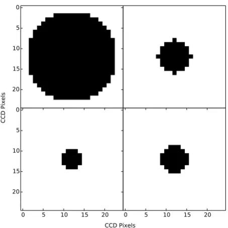
We developed a program to allow more flexible extraction according to the needs of K2 (as in for example Aigrain et al. 2015, although our extraction is more simple). The WCS infor-mation contained within the target pixel files was utilised to find the central pixel of the target (we found the WCS information to generally be accurate to within 1 pixel). An aperture was then set depending on the brightness of the target. We found through trial and error that apertures of radius 3, 4, 5 and 12 pixels, for targets withKeplermagnitude>16,<=16,<=13,<=10 respec-tively, produced good results while minimising the chance of blending with other targets in the window (see Fig.1for exam-ple apertures, within which each pixel is given full weighting). The aperture was recentred to the brightest pixel within its ini-tial position derived from the WCS coordinates (using the me-dian brightness of each pixel measured over the whole dataset). Apertures for objects withKeplermagnitudes<=10 were made particularly large due to the bleeding effect which can occur for these targets, and which covers large numbers of pixels. We lim-ited ourselves to 4 aperture sizes to allow easy recreation of the aperture when checking data without looking into the detail of the files. The relation of target magnitude to apparent size on the CCD is also not trivial, and can vary even for objects of the same magnitude. Hence a smaller number of fixed (larger) apertures avoid systematic issues that may be introduced by as-suming a tight magnitude-aperture size relation and for exam-ple letting the aperture size vary smoothly with magnitude. It is possible to recreate the used apertures by using the new header card “AP_RAD” provided in the data files (see Table 1). This is the squared aperture radius, and a pixel is within the aper-ture if (Xpixel−Xcentre)2+(Ypixel−Ycentre)2<AP_RAD, whereX andY are pixel coordinates in each axis. Once a raw lightcurve was available, background subtraction was performed using a background value determined by the median value of pixels out-side the aperture at each timestamp. Although a simple method, we found that this was generally robust. The use of the median avoids significant bias by other sources except in a small number of cases, especially as we do not consider cluster observations. The error on the background determination was found from the median of the absolute deviation from their median of the out
0
5
10
15
20
0 5 10 15 20
0
5
10
15
20
0 5 10 15 20
CCD Pixels
[image:3.595.319.546.72.299.2]CCD Pixels
Fig. 1.Example apertures for (clockwise from top left)Kepler magni-tude<=10,<=13,<=16,>16.
of aperture pixels, known as the “Median Absolute Deviation”. This was then added in quadrature along with the pixel errors inside the aperture to produce the extracted flux errors.
At∼2016 (BJD-2 454 833) during the Campaign 1 data, the spacecraft pointing changed significantly, resulting in movement of targets by over a pixel in some cases. As such we recalcu-lated the aperture centres after this time, using the same aperture shape.
2.2. Data detrending
The main source of systematic noise in K2 data is pointing drift, as has been pointed out previously (Vanderburg & Johnson 2014). This has been claimed to be from either pixel-to-pixel flat fielding errors or a combination of aperture losses and source crowding. We independently designed and implemented a method similar to that proposed by Vanderburg & Johnson (2014) in order to detrend our lightcurves, which removes all noise correlated with the pointing drift regardless of its source.
The row and column centroid positions were calculated for each timestamp. This was done through the relation
φx= nx
P x=0
x ny
P y=0
z(x, y) !
nx
P x=0
ny
P y=0
z(x, y)
(1)
wherez(x, y) is the flux at the pixel in rowxand columny,nxis the total number of pixels in each row,ny the total number of pixels in each column, andφx the resulting row centroid. The column centroid is calculated by changing each x to a y and vice versa.
At this stage points near a thruster firing event were cut, de-tected as those to either side of times where the point-to-point centroid shift was greater than 3 times the median point-to-point shift across the dataset. The centroid positions were then used to create a 2D surface of raw flux against position of the cen-troid on the CCD. An example such surface is shown in Fig.2. If the pointing drift had no impact on the flux, this surface should
0.15 0.10 0.05 0.00 0.05 0.10 0.15
Col Centroid (pix)
0.6 0.4 0.2 0.0 0.2 0.4 0.6
Row Centroid (pix) 0.20
0.15 0.10 0.05 0.00 0.05 0.10
Col Centroid (pix) 139000
139150 139300 139450 139600 139750 139900
[image:4.595.51.279.70.245.2]Flux on CCD (counts)
Fig. 2.Surface of raw flux against CCD position for EPIC201552917. The flux is split at 2016 (BJD-2 454 833), with the first segmentabove
and the second segmentbelow. Centroids have been offset to their re-spective means.
show no correlation. Instead, in the majority of cases a strong trend was seen. This trend was identified through binning the data into 10 evenly spaced bins in row and 10 in column, mak-ing 100 individual bins in total. The median flux in each bin was then taken and interpolated between linearly using the SciPy griddata function1(Jones et al. 2001), creating a smooth surface
mapping the variation caused by the observed centroid shifts. We used SciPy as it provides a versatile analysis tool for scientific work in Python. Bins containing fewer than 3 points were cut and not used for interpolation. The resulting surface was divided out, decorrelating the flux from spacecraft pointing and provid-ing a lightcurve in flux relative to unity. The griddata function can ignore some points if they have values inconsistent with the surface formed by the majority of input points; seeBarber et al. (1996) for a full description of the full algorithm, which forms the basis of griddata when used linearly and is more complex than can be concisely explained here. The surface at such points was defaulted to the nearest valid bin value. The correlation of an example lightcurve with centroid position is shown in Fig.3, both before and after detrending. In addition, outliers were re-moved by cutting data points where the centroid position was greater than 5 times the median distance from the median cen-troid position across the dataset. In all these situations medians rather than means and standard deviations were used in order to avoid the effects of large outliers. Example lightcurves, pre and post detrend, are shown in Figs. 4 and5. We note that in Campaign 1 in particular, some systematic noise remains after detrending, likely arising from instrumental effects as seen in the originalKeplerdata. Some such variation can be seen in the detrended lightcurve of Fig.4. Such variations can be seen in the Eigen lightcurves ofForeman-Mackey et al.(2015). The specific origin of the variations in K2 is at present poorly understood. We have not attempted to remove this variation in this work, as it does not correlate with the pointing drift.
At the same time as the previously mentioned pointing shift at∼2016 (BJD-2 454 833), the characteristics of the thruster fir-ing and associated spacecraft motion also changed. We do not know the underlying reason for this and so do not provide fur-ther detail. However, we adjusted for this effect by detrending the Campaign 1 lightcurves before and after the split separately.
1 http://www.scipy.org/, v0.15.
0.999 1.000 1.001 1.002 1.003 1.004
Detrended Flux (Relative Flux)
0.6 0.4 0.2 0.0 0.2 0.4 0.6
Flux Centroid (pix) 138800
139000 139200 139400 139600 139800 140000
Extracted Flux (Counts)
Fig. 3.Correlation of flux to CCD centroid position for the extracted
(bottom) and detrended (top) lightcurves of EPIC201552917. Row
cen-troid is shown in blue, column cencen-troid in red.
0.999 1.000 1.001 1.002 1.003 1.004
Relative Flux
1980 1990 2000 2010 2020 2030 2040 2050 2060 BJD - 2454833
139000 139200 139400 139600 139800 140000
[image:4.595.317.545.77.242.2]Raw Counts
Fig. 4. Extracted (bottom) and detrended (top) lightcurves for EPIC201552917, showing some systematic noise. The dashed line in-dicates the time where detrending was split.
This provided significantly improved lightcurves over results tried without a split, but has the disadvantage that long period variability can be removed. There was no need to perform such a split in Campaign 0, which contained no such characteris-tic change. We found that the above method worked well in most cases, but it has the weakness that intrinsic stellar vari-ability which occurs on a similar timescale to the dataset can be removed, if the spacecraft drift spuriously correlates with it. Detrending the Campaign 1 data in two segments means that this applies to variability on a shorter timescale, of order 35 days rather than the full dataset length of 79 days. We also note that large amplitude variability which dominates over the pointing noise can also be reduced in amplitude, should it correlate with the drift. The catalogue web pages show both extracted and de-trended flux, which will make such a reduction or blurring of a real signal evident if it has occurred.
[image:4.595.317.542.298.462.2]A&A 579, A19 (2015)
0.995 1.000 1.005 1.010
Relative Flux
1980 1990 2000 2010 2020 2030 2040 2050 2060 BJD - 2454833
108500 109000 109500 110000 110500 111000
[image:5.595.52.277.74.240.2]Raw Counts
Fig. 5. Extracted (bottom) and detrended (top) lightcurves for EPIC201809540, showing quasi periodic variability. The dashed line indicates the time where detrending was split.
2.3. Performance
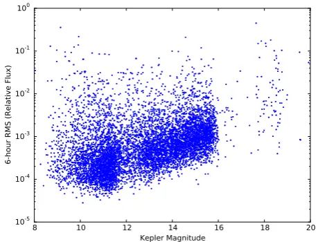
Having applied this detrending method to our set of K2 lightcurves we were in a position to test it’s overall perfor-mance as compared to the other methods available for K2 data (e.g. Aigrain et al. 2015; Vanderburg & Johnson 2014). For this purpose we have created a root median square (rms) plot, shown in Fig.6. This shows the 6-h performance of all detrended lightcurves from Campaign 0. We limited this test to Campaign 0 as the other available detrending methods for K2 data had only released up to at most Campaign 0 at the time of writing. Magnitudes are Kepler magnitudes and were taken from the “KEPMAG” header found within each data file. Rms values
were calculated as rms =hmedian(x−median(x))2i
1 2
, where xrepresents the array of 6-h binned flux values.
The plot shows a number of interesting characteristics. In particular is the slight turn up at the bright end, which is a result of the bleeding that can occur for brighter targets. In these cases it is likely that some flux was lost from the aper-ture. The distribution of magnitudes seen is largely a result of which proposed targets were selected for download from the spacecraft. In overall terms, the median 6-h rms value for our Campaign 0 detrended lightcurves was 5.39×10⁻⁴, with a “best” rms of 2.81×10⁻⁵. We downloaded the public Campaign 0 data fromVanderburg & Johnson(2014) to compare this result. The comparison was limited to lightcurves found in both sets of lightcurves (7691 in total). We cut points marked as being within thruster firing events, but otherwise leave the lightcurves as they are presented. Although this means that the comparison is not on precisely the same data points, it is instead between the lightcurves generated and published in both cases. As such it is a comparison of the lightcurves available, not the specific method. The median 6-h rms value for theVanderburg & Johnson(2014) lightcurves was 7.46×10⁻⁴, with a “best” rms of 3.52×10⁻⁵, implying that our method is performing comparatively. We are aware of one other published method for K2 data detrending, that ofAigrain et al.(2015). While Campaign 0 data were not avail-able for this method at the time of writing, the above rms values are comparable with the results shown by that method for the K2 Engineering dataset.
There are significant methodological differences between these and all other K2 detrending methods, for example in the aperture sizes and shapes used and methods of lightcurve extrac-tion as well as the detrending itself. As such, we explicitly do not
8 10 12 14 16 18 20
Kepler Magnitude 10-5
10-4
10-3
10-2
10-1
100
[image:5.595.316.546.75.250.2]6-hour RMS (Relative Flux)
Fig. 6.Root median square plot of all (i.e. variable and non-variable) Campaign 0 detrended lightcurves binned into 6-h bins. A small random noise on the magnitudes has been added for clarity.
claim that our method is better or worse than any other, merely performing comparably. Claiming improved performance would require significantly more work, and is largely irrelevant while the detrending methods are undergoing refinement, which is likely to happen for the duration of the K2 mission. The purpose of our method is to allow the rapid production of this catalogue so that it can be used reasonably soon after each data release.
2.4. Lightcurve file description
The detrended lightcurve data provided with this catalogue is presented in FITS format (Pence et al. 2010). We take the origi-nally available target pixel files from the MAST archive, and add to these several additional data columns and headers. These are detailed in Tables1and2. This allows all of the initial informa-tion provided by the K2 team to be preserved through the pro-cess. A description of the original files can be found at MAST.
3. Catalogue
The catalogue is presented in Table3, and the full version can be found online2. The fields in the table are described in Sect.3.2.
3.1. Variable detection and classification
Once the detrended lightcurve for each object was available, we proceeded to search for variability. If the amplitude of the lightcurve (i.e. half the full range) was less than 3 times the me-dian noise level the object was automatically discarded. For the remaining lightcurves a weighted, floating mean Lomb-Scargle (hereafter LS) periodogram (Lomb 1976;Scargle 1982) with an oversampling factor of 4 was created, following the method of Press & Rybicki(1989). Periods between 0.241 and 0.258 days were removed to avoid the 6-h thruster firing timescale. These limits were determined through experimentation. Each peri-odogram, alongside the detrended and extracted lightcurves, was then classified by eye, and a period selected if appropriate. It is possible that in some cases classified variability in the catalogue is in fact due to systematic instrumental noise, although this was avoided when possible (for example, if many lightcurves shared the same variation). This problem is most apparent for longer
2 http://deneb.astro.warwick.ac.uk/phrlbj/k2varcat/
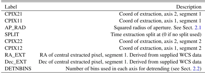
Table 1.Additional FITS headers in primary extension.
Label Description
CPIX21 Coord of extraction, axis 2, segment 1 CPIX11 Coord of extraction, axis 1, segment 1 AP_RAD Squared radius of aperture. See Sect.2.1 SPLIT Time extraction split at (0 if no split used) CPIX22 Coord of extraction, axis 2, segment 2 CPIX12 Coord of extraction, axis 1, segment 2 RA_EXT RA of central extracted pixel, segment 1. Derived from supplied WCS data Dec_EXT Dec of central extracted pixel, segment 1. Derived from supplied WCS data DETNBINS Number of bins used in each axis for detrending (see Sect.2.2)
Table 2.Additional data columns (in file extension 1).
Label Unit Description
APTFLUX Counts Extracted lightcurve
APTFLUX_ERR Counts Extracted lightcurve error APTFLUX_BKG Counts Calculated background APTFLUX_BKG_ERR Counts Calculated background error DETFLUX Relative Flux Detrended lightcurve DETFLUX_ERR Relative Flux Detrended lightcurve error CENT_ROW Pixel coordinates CCD Row Centroid CENT_COL Pixel coordinates CCD Column Centroid
Table 3.Catalogue.
EPIC ID Type Range Period Amplitude Proposal information
% d %
: : : : : :
201858862 AP 1.47 0.000000 0.00
201859140 QP 69.11 0.483664 4.19 1018 (RR Lyrae) 201859398 P 4.08 2.656481 1.02
201859496 AP 6.37 0.000000 0.00 1025 (AGN) 201859551 QP 3.67 9.374306 1.27
: : : : : :
Notes.When online, clicking on an object ID will show detailed plots, as well as allow download of it’s detrended lightcurve. An extract from the table is shown. The full table is available at the CDS.
period variation (greater than 20 days), and appears to be more common in Campaign 1 than Campaign 0.
After classification, period refinement was performed on ob-jects marked as eclipsing binary (EB), periodic (P) or quasi pe-riodic (QP). For P or QP lightcurves the LS periodogram was rerun with a higher oversampling factor of 20, over a range within ±10% of the previously marked period. The most sig-nificant peak within this range is then given as the catalogue period. For EBs a Phase Dispersion Minimisation periodogram was created (Stellingwerf 1978; Schwarzenberg-Czerny 1997), as these perform better on non-sinusoidal signals than do LS pe-riodograms. This was run with a frequency resolution of 10−5 (10−4for objects with periods below 1 d for efficiency reasons) over the same narrow range using 100 bins, and the most signif-icant peak taken, in order to refine the only approximate LS pe-riod for the EB systems.
We imposed a limit of 15 days on the periods of objects within Campaign 0, due to the 32 day data baseline. For objects in Campaign 1, a limit of 20 days was imposed. The baseline for Campaign 1 (79 days) could allow longer periods, but due to
the detrending method used, and specifically the splitting of the data into separate halves for detrending, signals on longer peri-ods would not be robust. This does not apply to eclipses how-ever, and as such no period limit was imposed on EB systems. Some EBs are classified without a period. In these cases either the period was too long to provide multiple eclipses, or for some other reason the period was uncertain. These generally represent the longest period objects in the catalogue, and so should be of special interest.
A&A 579, A19 (2015)
Lightcurves are presented after extraction using data release 2 and the WCS information, with the implied reduced chance of blending. Classification was not repeated due to the significant time involved in performing it.
3.2. Fields
1. EPIC ID
ID of target from the EPIC catalogue. Spans 201122454– 210282474.
2. Type
Lightcurves were classified by eye as eclipsing binary (EB), periodic (P), quasi-periodic (QP), or aperiodic (AP). Periodic classification implies a sinusoidal variation of constant pe-riod and amplitude. Quasi-pepe-riodic objects have amplitude or period variations, or a lightcurve non-sinusoidal in shape. Aperiodic objects showed no periodicity (though an object may also be classified as AP if it had no dominant peri-odicity). In many cases these objects may be periodic but with periods greater than 15 days for Campaign 0 or 20 days for Campaign 1, a limit imposed due to the data baseline (and the split used when detrending Campaign 1 data). Users should be aware that objects which should be classified as P can be misclassified as QP due to noise, and more rarely vice versa.
3. Range
The lightcurves were binned into 10 point wide bins and the median of each bin found. The range given is the maximum bin less the minimum, in flux units relative to the overall data median. In some cases outliers or remnant noise can af-fect this calculation, leading to ranges larger than are shown. Spans 0.03−429.85%.
4. Period
The most significant peak from a Lomb-Scargle peri-odogram, for objects classified as P or QP. For eclips-ing binaries the peak was found useclips-ing Phase-Dispersion Minimisation (see Sect.3.1). Where possible the true period rather than an alias is given, even if the aliases were more sig-nificant. Zero for AP objects. No periods larger than 15 days for Campaign 0 and 20 days for Campaign 1 are shown to avoid spurious detections due to the data baseline. For the same reason, while we report periods up to these limits those within ∼5 days of them should be treated with some cau-tion. However, EB objects have no period limits imposed. Spans 0−59.889024 days.
5. Amplitude
The semi-amplitude of the lightcurve at the stated period, for objects classified P or QP. This was calculated through phase-folding the lightcurve, binning it into 40 evenly spaced bins, then taking the median of each bin. The semi-amplitude represents half of the maximum minus minimum bin value, in flux units relative to the overall data median. Short period objects will show reduced amplitude due to the cadence of the observations. For EB objects the number of bins was increased to 300, to improve detection of narrow eclipses. The resulting eclipse depth is then given directly (i.e. not
halved as is the case for other objects). Zero for AP objects. Spans 0−96.78%.
6. Proposal information
Guest Observer proposals relating to the object. Only vari-able star related proposals are shown. If possible, the specific variable types which each proposal is related to are given in brackets.
4. Conclusion
We have presented a catalogue of variable stars and eclipsing binaries from K2 Campaigns 1 and 0. This catalogue will be updated with each K2 data release, which we hope will provide a valuable resource for users interested in these objects. Detrended lightcurves for catalogue objects are also available, and compare favourably to already available detrending methods. We hope to make available detrended lightcurves for objects not found in the catalogue at a future date.
Acknowledgements. We thank the anonymous referee for a detailed review of the manuscript. The data presented in this paper were obtained from the Mikulski Archive for Space Telescopes (MAST). STScI is operated by the Association of Universities for Research in Astronomy, Inc., under NASA contract
NAS5-26555. Support for MAST for non-HST data is provided by the NASA Office of
Space Science via grant NNX13AC07G and by other grants and contracts. The authors would like to thank Thomas Marsh for use of his periodogram generating Python code.
References
Aigrain, S., Hodgkin, S. T., Irwin, M. J., Lewis, J. R., & Roberts, S. J. 2015,
MNRAS, 447, 2880
Armstrong, D. J., Osborn, H. P., Brown, D. J. A., et al. 2014, ArXiv e-prints [arXiv:1411.6830]
Banyai, E., Kiss, L. L., Bedding, T. R., et al. 2013,MNRAS, 436, 1576
Barber, C. B., Dobkin, D. P., & Huhdanpaa, H. 1996,ACM transactions on
math-ematical software, 22, 469
Chaplin, W. J., Basu, S., Huber, D., et al. 2013,ApJS, 210, 1
Conroy, K. E., Prsa, A., Stassun, K. G., et al. 2014,PASP, 126, 914
Crossfield, I. J. M., Petigura, E., Schlieder, J., et al. 2015,ApJ, 804, 10
Debosscher, J., Blomme, J., Aerts, C., & De Ridder, J. 2011,A&A, 529, A89
Foreman-Mackey, D., Montet, B. T., Hogg, D. W., et al. 2015, ApJ, submitted [arXiv:1502.04715]
Holdsworth, D. L., Smalley, B., Kurtz, D. W., et al. 2014,MNRAS, 443, 2049
Howell, S. B., Sobeck, C., Haas, M., et al. 2014,PASP, 126, 398
Jones, E., Oliphant, T., Peterson, P., et al. 2001, SciPy: Open source scientific tools for Python, online; accessed 2015-04-14
Lomb, N. R. 1976,Astrophys. Space Sci., 39, 447
McQuillan, A., Aigrain, S., & Roberts, S. 2012,A&A, 539, A137
Nardiello, D., Bedin, L. R., Nascimbeni, V., et al. 2015,MNRAS, 447, 3536
Pence, W. D., Chiappetti, L., Page, C. G., Shaw, R. A., & Stobie, E. 2010,A&A, 524, A42
Press, W. H., & Rybicki, G. B. 1989,ApJ, 338, 277
Prsa, A., Batalha, N., Slawson, R. W., et al. 2011,AJ, 141, 83
Reinhold, T., Reiners, A., & Basri, G. 2013,A&A, 560, A4
Scargle, J. D. 1982,ApJ, 263, 835
Schwarzenberg-Czerny, A. 1997,ApJ, 489, 941
Stassun, K. G., Pepper, J. A., Paegert, M., De Lee, N., & Sanchis-Ojeda, R. 2014,
ArXiv e-prints [arXiv:1410.6379]
Stellingwerf, R. F. 1978,ApJ, 224, 953
Stello, D., Compton, D. L., Bedding, T. R., et al. 2014,ApJ, 788, L10
Uytterhoeven, K., Moya, A., Grigahcène, A., et al. 2011,A&A, 534, A125
Vanderburg, A., & Johnson, J. A. 2014,PASP, 126, 948
Vanderburg, A., Montet, B. T., Johnson, J. A., et al. 2015,ApJ, 800, 59