A Thesis Submitted for the Degree of PhD at the University of Warwick
Permanent WRAP URL:
http://wrap.warwick.ac.uk/89770
Copyright and reuse:
This thesis is made available online and is protected by original copyright. Please scroll down to view the document itself.
Please refer to the repository record for this item for information to help you to cite it. Our policy information is available from the repository home page.
Modelling and Optimization of Remote Laser Welding Galvanized
Steels Using Statistical Methodologies
by
Yanglin Shi
Supervisor: Professor Stuart Barnes
Abstract
This thesis is written under the circumstance of “Remote Laser Welding (RLW) System for Eco & Resilient Automotive Factories” project, of which goals are to configure, integrate, test and validate application of RLW system in automotive assembly line. The goal of this study is to identify the RLW process window and optimal parameters setting for four different material stack-ups in the configuration of lap joint.
One-Factor-at-A-Time method is used to determine the process window in which sound welds, free from visible defects such as spatter, cut-through, burn-through and insufficient weld, are produced. One step further, sound welds are transversely cross-sectioned and geometric profiles (top concavity, interface width, penetration and bottom concavity) are measured and compared to industrial standards. Eventually, it is determined that within power [3, 4] kW, speed [2.5,5.5] m/min, gap [0.15, 0.30] mm, welds fulfilling visual and non-visual requirements could be produced for stack-up of DX56D+Z 1.00 mm plus DX54D+Z 1.00 mm.
Paired mean hypothesis test between stack-up of 0.75 mm DX56D+Z plus 1.00 mm DX54D+Z and stack-up of 0.75 mm DX56D+Z plus 1.80 mm DX56D+Z is performed with the objective of testing whether lower thickness is a significant factor affecting the process. The results reveal insignificance. The process modelling is therefore simplified to focus on the stack-up with greatest lower thickness. Thanks to this result, it significantly reduces the total experimental work.
My gratitude also goes to Professor Kevin Neailey, Professor Stuart Barnes and Jennifer Kirkwood. Many thanks to Professor Stuart and Kevin for giving good advice. Great thanks to Jennifer Kirkwood for assisting me in every process of getting experimental work done and thesis written.
My sincere thanks also go to Mr David Moseley, Mr David Williams and Mr David Cooper. All of them, the kindest and most professional individuals I have ever met, helped me through the process of writing this thesis. Gratitude also goes to colleagues Abhishek Das, Dr Pasquale Franciosa and Selim Yilmazer. Should there not be their support, this thesis could never have been finally finished. In addition, great thanks to Gabriele Gattere who was an exchange student from University of Polimi Milano in Italy with good knowledge on laser welding and Andrés Ortiz Arroyave who worked on this project for his Master’s degree before me. Without any of them, I could not have finished this thesis.
Contents
Abstract ... i
Acknowledgement ... ii
Contents ... iii
Abbreviation ... v
List of Figures ... vi
List of Tables ... xviii
1. Introduction ... 1
2. Research background ... 7
2.1 RLW system ... 7
2.1.1 Laser source ... 8
2.1.2 COMAU Smart Laser ... 11
2.1.2.1Robotic system and scanning head ... 11
2.1.2.2Controlling system ... 12
2.2 WMG TSB project ... 13
2.3 Industrial weld quality definition ... 14
3. Literature review ... 26
3.1 Principle of Laser ... 26
3.2 Evolution of laser application in automotive industry ... 27
3.3 Working principles of RLW... 28
3.4 Conduction-limited vs Keyhole wleding ... 30
3.5 Zinc degassing solutions ... 32
3.6 Process modelling and optimization ... 35
4. Methodologies ... 51
4.1 Problem-solving roadmap ... 51
4.2 Identification of process factors ... 54
4.3 Methodology for process window identification ... 56
4.4 Paired mean test ... 59
6.2.2 Analysis and discussion of the results ... 116
6.3 Process modelling campaign-RSM ... 118
6.3.1 Objectives and experimental design... 118
6.3.2 Development of mathematical models ... 122
6.4 Optimization results for four stack-ups ... 128
6.4.1 Optimization formulation for stack-up 0.75 mm-1.80 mm ... 128
6.4.2 Optimization formulation for stack-up 0.75 mm-1.00 mm ... 133
6.4.3 Optimization formulation for stack-up 0.75 mm-0.70 mm ... 137
7. Conclusions and discussion ... 142
7.1 Conclusions ... 142
7.2 Discussion ... 143
Abbreviation
Abbreviation Full name
BIW Body-in-White
OEM Original Equipment Manufacturer
PLW Proximity Laser Welding
RLW Remote Laser Welding
RSW Resistance Spot Welding
SU Stack-up
TSB Technology Strategy Board
HAZ Heat Affected Zone
WMG Warwick Manufacturing Group
IPG IPG Photonics Corporate
COMAU
COnsorzio MAcchine Utensili, Italian company, part of Fiat Group
ABSL Application BoxSmart Laser
Figure 2. 1 WMG RFLW system (Source: COMAU) ... 8
Figure 2. 2 IPG YLR-4000 laser source with 8 modules inside ... 10
Figure 2. 3 A module of IPG YLR-4000 laser (Source : IPG) ... 11
Figure 2. 4 Robotic arm and scanning head (Source: COMAU) ... 12
Figure 2. 5 Control box of the RLW system (Source : COMAU) ... 13
Figure 2. 6 Correlation between four characteristics and Ford KPIs ... 16
Figure 2. 7 Partial penetration mode of laser welding ... 17
Figure 2. 8 Full penetration mode of laser welding ... 17
Figure 2. 9 Length (Source: Ford Standards) ... 18
Figure 2. 13 Spatter (from Arroyave, A.O., 2012) ... 22
Figure 2. 14 Cut-through ... 23
Figure 2. 15 Burn-through ... 24
Figure 2. 16 Weld discontinuity (from Arroyave, A.O., 2012) ... 24
Figure 3. 1 Basic components of a laser construction, from (Steen and Mazumder, 2010) ... 27
Figure 3. 2 Laser application development for automotive industry, from (Mori et al., 2010) ... 28
Figure 3. 3 An example of RLW system (adapted from (Kang et al., 2011)).... 29
Figure 3. 4 Plasma shielding at high laser power [0.5, 6] kW; speed= 2m/min, mild steel, from Grupp et al., 2003 ... 30
Figure 3. 5 Conduction welding mode, from (Steen and Mazumder, 2010) ... 31
Figure 3. 6 Keyhole welding mode, from (Steen and Mazumder, 2010)... 31
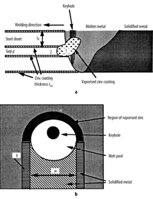
Figure 3. 7 Schematic picture of laser welding zinc-coated steel with a small
gap between the sheets for exhausting of the high-pressure zinc vapour: a.
Figure 4. 2 All the needed to be considered process parameters for a laser
welding systems, adapted from (Steen and Mazumder, 2010) ... 54
Figure 4. 3 Process to identify the process window ... 58
Figure 4. 4 Three factor three level Box-Behnken Design ... 60
Figure 5. 1 RLW system in Warwick Manufacturing Centre ... 68
Figure 5. 2 Laser beam quality measurement ... 68
Figure 5. 3 Internal designed fixture for the study ... 69
Figure 5. 4 Dimensions of a sample ... 75
Figure 5. 5 Shims in yellow used in this study to create the gap ... 76
Figure 5. 9 Sample Preparation System Buehler Pheonix 4000 ... 78
Figure 5. 10 Optical microscope Leica DM 4000 M ... 78
Figure 5. 11 Example of sample cross section. ... 79
Figure 5. 12 Measured variables: top concavity, penetration, interface width and
gap ... 80
Figure 5. 13 Measured variable: bottom concavity (applicable case) ... 80
Figure 5. 14 Measurement of penetration ... 81
Figure 5. 15 Cross-section of five pieces under optical microscope: speed=3.00
m/min; power= 4.00 kW; gap=0.20 mm ... 82
Figure 5. 16 Mean and variation value of top concavity: speed=3.00 m/min;
power= 4.00 kW; gap=0.20 mm ... 83
Figure 5. 17 Mean and variation value of interface width: speed=3.00 m/min;
power= 4.00 kW; gap=0.20 mm ... 84
Figure 5. 18 Mean and variation value of penetration: speed=3.00 m/min;
power= 4.00 kW; gap=0.20 mm ... 84
Figure 6. 6 Schematic figure of welding behaviour when power=3.00 kW ... 95
Figure 6. 7 Schematic figure of welding behaviour when power=2.00 kW ... 97
Figure 6. 8 Overlapped region in yellow at power=2.00 kW, 3.00 kW, and 4.00
kW. With right choice of combination of gap and speed, sound weld joints
could be produced. ... 98
Figure 6. 9 (a) Process parameters : Power =2.00 kW, Speed=4.00 m/mim,
Gap=0.20 mm ; Geometric dimensions: Top concavity =305.01 ૄܕ,
Interface width= 1048.04 ૄܕ , Penetration= 186.26 ૄܕ ,Bottom
concavity=0; Status=NOK (insufficient penetration) ... 99
Figure 6. 10(b) Process parameters: Power=2.50 kW, Speed=4.00 m/min,
Gap=0.20 mm ; Geometric dimensions: Top concavity=358.56 ૄܕ,
Interface width= 1549.99 ૄܕ; Penetration= 644.94 ૄܕ. Status=Pending
(considering standard deviation of top concavity, could not be decided) 100
Figure 6. 12 (d) Process parameters : Power=3.50 kW, Speed=4.00 m/min,
Gap=0.20 mm; Geometric dimensions: Top concavity =242.14 ૄܕ,
Interface width=1559.96 ૄܕǡ Penetration=984.88 ૄܕ; Status=OK ... 100
Figure 6. 13 (e) Process parameters: Power=4.00 kW, Speed=4.00 m/min,
Gap=0.2 mm (e); Geometric dimensions: Top concavity=162.98 ૄܕ,
Interface width=1424.03 ૄܕ, Penetration=954.61 ૄܕ full penetration,
Bottom concavity= 172.29 ૄܕ; Status= OK ... 100
Figure 6. 14 Scattering plot of bead profile geometric dimensions: Gap=0.20
mm, Speed=4.0 m/min, Power= [2.0, 4.0] kW. ... 102
Figure 6. 15 Regression analysis of bead profile geometric dimensions:
Gap=0.20 mm, Speed=4.0 m/min, Power= [2.0, 4.0] kW. ... 103
Figure 6. 16 (1) Power=4.00 kW, Speed=2.50 m/min, Gap=0.20 mm; Top
concavity=277.07 ૄܕ, Interface width= 1478.53 ૄܕ, Penetration =670.56
ૄܕ, Bottom concavity=279.43 ૄܕ. Status=OK ... 106
Figure 6. 17 (2) Power=4.00 Kw, Speed=3.00 m/min, Gap=0.20 mm; Top
Penetration=782.32 ૄܕ, Bottom concavity=172.29 ૄܕ. Status=OK .... 106
Figure 6. 20 (5) Process parameters: Power=4.00 kW, Speed=4.50 m/min,
Gap=0.2 mm; Top concavity=missing, Interface width=1258.25 ૄܕ ,
Penetration=849.92ૄܕ, Bottom concavity=112.92 ૄܕ. Status= OK ( Top
concavity information missing)... 107
Figure 6. 21 (6) Process parameters: Power=4.00 kW, Speed=5.00 m/min,
Gap=0.20 mm; Top concavity= 246.80 ૄܕ, Interface width= 1443.65 ૄܕ,
Penetration= 533.20 ૄܕ, Bottom concavity=0. Status=OK ... 107
Figure 6. 22 (7) Process parameters: Power=4.00 kW, Speed=5.50 m/min,
Gap=0.20 mm; Top concavity=286.38 ૄܕ, Interface width=1541.36 ૄܕ,
Penetration=449.30ૄܕ, Bottom concavity=0; Staust=OK ... 107
Figure 6. 23 (8) Process parameters: Power=4.00 kW, Speed=6.00 m/min,
Figure 6. 24 (9) Process parameters: Power=4.00 kW, Speed=6.50 m/min,
Gap=0.20 mm; Top concavity=305.01 ૄܕ, Interface width= 1275.91 ૄܕ,
Penetration=318.98 ૄܕ, Bottom concavity= 0; Status=NOK (dangerous
top concavity and penetration considering standard deviation) ... 108
Figure 6. 25 (10) Process parameters: Power=4.00 kW, Speed=7.00 m/min,
Gap=0.20 mm; Top concavity= 251.46 ૄܕ, Interface width= 1115. 26 ૄܕ,
Penetration= 211.87 ૄܕ, Bottom concavity= 0; Status=NOK (insufficient
penetration) ... 108
Figure 6. 26 (11) Process parameters: Power=4.00 kW, Speed=7.50 m/min,
Gap=0.20 mm; Top concavity= 423.75 ૄܕ, Interface width=1196.74 ૄܕ,
Penetration= 179.34 ૄܕ, Bottom concavity=0; Status=NOK (Excessive
top concavity, insufficient penetration)... 108
Figure 6. 27 (12) Process parameter: Power=4.00 kW, Speed=8.00 m/min,
Gap=0.20 mm; Top concavity= 260.77 ૄܕ, Interface width= 905. 70 ૄܕ,
Penetration= 60.54 ૄܕ, Bottom concavity= 0; Status= NOK (insufficient
penetration) ... 108
Figure 6. 28 Scattering plot of bead profile geometric dimensions: Gap=0.20
mm, Power=4 kw, Speed= [2.5, 8] m/min ... 111
(Spatter, cut-though) ... 113
Figure 6. 33 Power=4.00 kW; Speed= 4.00 m/min; Gap=0.15 mm, Status=OK
... 113
Figure 6. 34 Power=4.00 kW; Speed= 4.00 m/min; Gap=0.20 mm, Status=OK
... 114
Figure 6. 35 Power=4.00 kW; Speed= 4.00 m/min; Gap=0.25 mm, Status=OK
... 114
Figure 6. 36 Power=4.00 kW; Speed= 4.00 m/min; Gap=0.30 mm, Status=OK
... 114
Figure 6. 37 Power=4.00 kW; Speed= 4.00 m/min; Gap=0.35 mm, Status
Figure 6. 40 3D graph to show the model of top concavity, gap at 0.20 mm .. 124
Figure 6. 41 Contour graph to show the model of top concavity, gap at 0.20 mm
... 124
Figure 6. 42 3D graph to show the model of penetration, Gap at 0.20 mm ... 126
Figure 6. 43 Contour graph to show the model of penetration, Gap at 0.20 mm
... 126
Figure 6. 44 Optimum of desirability of stack-up 0.75 mm-1.80 mm ... 132
Figure 6. 45 Optimum of penetration on plane of power and speed for stack-up
0.75 mm-1.80 mm ... 132
Figure 6. 46 Overlay Plot of Optimum setting gap at 0.15mm for stack-up 0.75
mm-1.80 mm ... 132
Figure 6. 47 Optimum of desirability of stack-up 0.75 mm-1.00 mm ... 136
Figure 6. 48 Optimum of penetration on plane of power and speed for stack-up
0.75 mm-1.00 mm ... 136
Figure 6. 49 Overlay Plot of Optimum setting gap at 0.18 mm for stack-up 0.75
Figure 7. 2 Cross-section 2 of trial 1 ... 146
Figure 7. 3 Cross-section 3 of trial 1 ... 146
Figure 7. 4 Cross-section 4 of trial 1 ... 146
Figure 7. 5 Cross-section 5 of trial 1 ... 147
Figure 7. 6 The mean value and standard deviation of top surface concavity 147 Figure 7. 7 The mean value and standard deviation of interface width ... 147
Figure 7. 8 The mean value and standard deviation of Penetration ... 147
Figure 7. 9 The mean value and standard deviation of bottom surface concavity ... 148
Table 2. 2 Operating range of every axis of the robot (Source : COMAU,
Appendix C) ... 12
Table 2. 3 Permissible material thickness combinations for DX54 (Source: TSB
report) ... 14
Table 3. 1 Comparison among the common modelling/optimizing techniques for
laser welding (adapted fromBenyounis and Olabi (2008)) ... 43
Table 3. 2 Summary of all the mentioned studies of modelling and optimizing
for laser welding ... 45
Table 3. 3 Summary of detailed information of the studies for modelling and
optimizing of laser welding ... 46
Table 5. 2 Chemical composition of DX56D+Z, DX54D+Z, DX52D+Z and
DX53D+Z. ... 70
Table 5. 3 Permissible deviation of DX56D+Z, DX54D+Z, DX52D+Z and DX53D+Z ... 71
Table 5. 4 Mechanical properties of DX56D+Z ... 72
Table 5. 5 Mechanical properties of DX54D+Z ... 72
Table 5. 6 Mechanical properties of DX52D+Z ... 73
Table 5. 7 Mechanical properties of DX53D+Z ... 74
Table 5. 8 Mean and variation value of measured variables: speed=3.00 m/min; power= 4.00 kW; gap=0.20 mm ... 83
Table 5. 9 Specification of the metallographic treatment for weld joints ... 85
Table 6. 1 Experimental design for process window identification: ... 92
Table 6. 2 Experimental design for process window identification: ... 94
Table 6. 3 Experimental design for process window identification: ... 96
Table 6. 10 Factors and experimental design levels ... 118
Table 6. 11 Three factor Box-Behenken Design with 3 centre points and the
experimental results ... 120
Table 6. 12 Fit analysis for top concavity modelling ... 122
Table 6. 13 ANOVA table for Top concavity ... 123
Table 6. 14 Fit analysis for interface width modelling ... 124
Table 6. 15 ANOVA analysis for interface width... 125
Table 6. 16 Fit analysis for penetration ... 125
Table 6. 17 ANOVA analysis for penetration ... 125
which right quality weld joints without defects according to industrial standards
could be produced. Secondly, within the identified process window, the optimal
condition under which with least power and fastest speed, meanwhile the right
quality of weld joints is achieved is to be investigated and concluded.
Figure1. 1 Lap joint configuration (from Ford Welding Standards, Appendix F)
Table1. 1 Four different stack-ups for door of interest
Upper
Upper
Lower
SU3 DX56D+Z 0.75 mm DX54D+Z 1.00 mm
SU4 DX56D+Z 0.75 mm DX53D+Z 0.70 mm
The reasons why galvanized steel and RLW have been gaining continuous attention
in automotive industry are investigated. In automotive industry, durability
improvement and fuel consumption reduction have been the main pursuits these
years. The corrosion resistance of material contributes to the improvement of
durability, and weight reduction helps to decrease fuel consumption (Zhao et al.,
2012,Mei et al., 2009, Chen et al., 2012). Galvanized steel, in possess of the merit of
better corrosion resistance than mere alloy steel without coating, has been
increasingly used as BIW panels. Meanwhile, RLW technique, due to its
characteristics of non-contact and smaller weld area, enables those panels to be
designed with smaller flanges, consequently it even reduces the overall weight of the
BIW.
In BIW assembly line, different joining processes have been used to join metallic
components, iron-carbon alloys with various shapes and geometries. The joints shall
have sufficient tensile strength, stiffness and be free from defects such as cracks and
spatters for the sake of surface aesthetics. Meanwhile, considering manufacturing
engineering and plant management, the joining processes are required to deliver high
shorter cycle time. It also has many other advantages e.g. deep penetration, high
speed, small heat affected zone (HAZ), fine welding bead quality, low heat input,
fibre beam delivery and no direct contact (Zhao et al., 2012, Mei et al., 2009, Chen et
al., 2012). However, PLW is much more expensive than RSW and has the risks of
collision and contamination of the scanner.
With the development of disk and fibre laser, RLW has emerged as another
alternative. By the application of long focal lenses, RLW welding scanner can be set
at a distance of more than 1 m away from the workpiece instead of standing off at a
distance in the order of magnitude of centimetres. This merit helps to eliminate the
risk of collision and contamination. In addition, by tilting two galvanometric mirrors
in the laser welding scanner, the laser beam could cover a wide working area at high
speed (Grupp et al., 2003, Kang et al., 2011). Benefit from it, the repositioning time
of RLW is significantly shortened, limiting to several milliseconds compared to
several seconds of RSW and PLW. Despite all the advantages, some difficulties still
studied widely in academia, and different solutions have been proposed. One
direction focuses on pre-treatment of the welding surfaces by either adding additional
elements (Baardsen, 1975) or removing zinc-coating (Pennington, 1987) to eliminate
the vaporization phenomenon, which seems to lack the feasibility of industrial
application. Another direction focuses on adjusted laser beam such as dual focus
beam (Banas and Doyle, 1987) , oscillated laser beam (Stol and Martukanitz, 2004) ,
fast frequency modulation of laser power (Schmidt et al., 2008) and etc. The other
direction concentrates on creating a gap between the two metal sheets for the zinc to
degas. (Rito et al., 1988) suggested to create the gap by loose contact or inserting
spacers. (Petrick, 1990) used pre-stamped projection technique to create V-shape
tabs in the lower part which acts as the required gap. (Colombo et al., 2012) believed
that dimplings that are protrusions from the lower sheet, created by laser, had an
advantage over others as it shows the industrial feasibility of mass production.
In this study, the chosen solution is to create a gap using shims as illustrated in
Figure 1. 2. In order to increase the consistency and reduce the variation of the gap, a
specifically designed fixture is used and will be introduced in detail in Chapter
5-Experimental Set-up. One-Factor-at-a-Time method is applied to figure out the
process window, and then Response Surface Methodology (RSM) is used to establish
the correlation models between process parameters and weld-joint geometric
Figure 1. 2 Shims in yellow to create the gap between two coupons
When it comes to establishing correlation models between process parameters and
process outputs and the optimal process parameters, a great number of studies have
been carried out in literature. Different methodologies such as RSM (Benyounis et al.,
2005a, Benyounis et al., 2005b, Manonmani et al., 2007, Rizzi et al., 2011, Khan et
al., 2011, Zhao et al., 2012, Padmanaban and Balasubramanian, 2010), Artificial
Neural Network Method (Vitek et al., 1998, Jeng et al., 2000), Taguchi methodology
(Sathiya et al., 2011, Lee et al., 2006, Pan et al., 2005, Anawa and Olabi, 2008, Olabi
and Anawa, 2006) and etc. were applied. In this study, thanks to RSM’s advantages
over other methods in this context, it is chosen as the methodology for correlation
modelling and optimization.
consumption and deliver weld joints with “right” quality. Thanks to the proposed
problem-solving roadmap in Chapter 4-Methodology, this study accomplishes the
goals by conducting experiments on one material stack-up and the correlation models
could be shared among four stack-ups. It helps reduce tedious repeats of
experimentation.
In the end, it is concluded that within power [3, 4] kW, speed [2.5,5.5] m/min, gap
[0.15, 0.30] mm, weld joints fulfilling visual and non-visual requirements could be
soundly produced for stack-up of DX56D+Z 1.00 mm plus DX54D+Z 1.00 mm. For
stack-up of 0.75 mm DX56D+Z plus 1.8 mm DX 54D+Z , the optimal results are
speed at 3.30 m/min, power at 3.80 kW, and gap at 0.15 mm; For stack-up of 0.75
mm DX56D+Z sheet plus 1.00 mm DX52D+Z or 1.00 mm DX 54D+Z, optimal
results are: speed at 3.86 m/min, power at 3.19 kW, and gap at 0.18 mm; For
stack-up 0.75 mm DX56D+Z plus 0.70 mm DX53D+Z, optimal results are: speed at 4.65
been carried out in Warwick Manufacturing Group (WMG) with the objective of
defining RLW process engineering guidelines. These two projects utilize the same
RLW system located in Warwick manufacturing centre, University of Warwick. The
system integrates an IPG 4 kW laser source and a COMAU Smartlaser. Thanks to the
results shared from TSB, tremendous useful information is ready to use.
In this chapter, the architecture of RLW and major conclusions of TSB project
relevant to this study are introduced. Afterwards, automotive weld quality definition
of lap-joint welds is presented.
2.1
RLW system
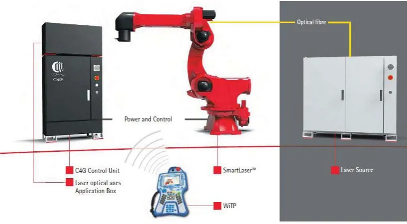
The RLW system, integrating an IPG 4 kW laser source and a COMAU Smartlaser
in a cell is illustrated in Figure 2. 1. The laser source is a 4 kW high brightness fibre
laser and COMAU Smartlaser is an industrial robot with a 4-axis robotic arm
in the weld pool. An additional air-knife is used to blow away the melted material
[image:31.595.115.524.185.410.2]particles and prevent the optics from contamination.
Figure 2. 1 WMG RLW system (Source: COMAU)
2.1.1 Laser source
The Ytterbium Fibre Laser (YLR-4000) from IPG Photonics could emit 4 kW power
at maximum. The power is supplied by 8 modules. Within each module, an array of
pump diodes launch electromagnetic radiation at 960 nm into the delivery fibre,
which transmits the 960 nm radiation into another section of the same fibre in which
Table 2. 1 Technical specification of IPG YLR-4000
IPG YLR-4000 (Yetterbium Fibre
Laser)
Laser wavelength 1070 nm
Available laser power 4 kW
Operating mode Continuous wave
Number of power module 8
Feed fibre diameter 200μm
M2
Source (at output of delivery fibre) =21.4
Cooling mode Water
Note: M2, known as beam quality factor, represents the degree of variation of a beam
from an ideal Gaussian beam. It reflects how well a collimated laser beam can be
[image:33.595.169.470.258.645.2]focused to a small spot, or how well a divergent laser source can be collimated.
Figure 2. 3 A module of IPG YLR-4000 laser (Source : IPG)
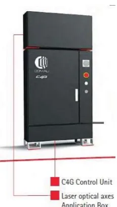
2.1.2 COMAU Smart Laser
2.1.2.1 Robotic system and scanning head
COMAU Smartlaser integrates a classical NH1 (COMAU’s internal code) 4-axis
robot (called anthropomorphic arm, Arm 2, in Figure 2. 4) with an optical arm
(called focusing and addressing arm, Arm 1, in Figure 2. 4) that is used to direct the
laser beam to the workpiece in high dynamics. The focusing of the laser beam could
be achieved at a range of distance between 750 mm and 1100 mm through adjusting
lens positions in arm 2. This adjusting mechanism is realized through utilizing an
electronic cam controlled by 3 motorized axes. Thanks to this solution, the focusing
axis has low inertia and can move at the speed of 4 m/s at maximum and the
acceleration could be as high as 8 times of gravitational acceleration (8g). After the
Figure 2. 4 Robotic arm and scanning head (Source: COMAU)
Table 2. 2 Operating range of every axis of the robot (Source : COMAU, Appendix C)
The magnification ratio of the optical chain is 3. Therefore, with the feed fibre
diameter of 200 μm, the laser beam waist diameter is 600 μm.
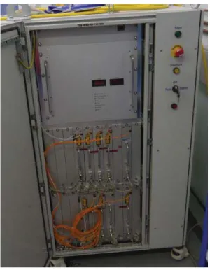
2.1.2.2 Controlling system
The controlling system has two separate modules. C4G is a typical COMAU control
Antropomorphic
Arm
Figure 2. 5 Control box of the RLW system (Source : COMAU)
2.2
WMG TSB project
In TSB project, useful guidelines for applying RLW technique to volume
manufacturing have been concluded through thousands of experiments and tests. In
this section, the guidelines regarding welding zinc-coated steels, which are closely
relevant to this study, are highlighted. The TSB report is attached as Appendix D in
this thesis.
Guideline 3: Any combination of the following grades of steel can be readily and
acceptably welded: DC04, DC05, DX54, DX55, HSLA, BH (up to 260), XF (up to
350), DP (up to 600), boron steels (up to 1200), 304, EN8 EN16, EN30.
Guideline 4: For DX54, the thickness combinations in green, shown in Table 2. 3,
are able to produce good weld joints in term of lap shear strength.
Table 2. 3 Permissible material thickness combinations for DX54 (Source: TSB report)
Guideline 5: Material stack combinations where one or both materials are coated
with zinc are readily weldable if a suitable interface gap is maintained, and the
optimum value of the gap is 0.18 mm.
Guideline 6: The allowed incident angle of the laser beam to workpieces surface is
30 degrees from perpendicular.
2.3
Industrial weld quality definition
According to (Juran et al., 1999), fitness for intended use to customer’s satisfaction is
0.7 1 1.5 1.7 2 2 (boron) 3
0.7 4.6 5.1 5.8 5.8 6
1 5.1 7.4 7.7 6.2
1.5 7.8 11.4
1.7 5.5 12.7
2 5.8 8.2 17.8
2 (boron) 6 9.4
3 17.2
Material Capability: DX54: Expected Lap shear strength
Top
within its entire life cycle. The appearance of the weld is an important contributor for
perceived quality and homogeneous welds not only reduce the risk of corrosion but
also give an impression of premium quality and high technology to the customers.
Strength, reliability and durability need to be tested. The tests could either be
destructive or non-destructive. Appearance could be subjectively evaluated.
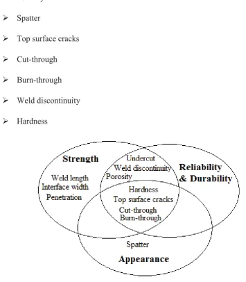
In Ford internal standards (Appendix F), the above mentioned characteristics could
be inferred from macro evaluation or metallographic assessment of weld bead, which
means there are correlations (in Figure 2. 6 ) between those characteristics and the
KPIs defined in the Ford standards. The defined KPIs are:
¾ Weld length
¾ Interface width
¾ Porosity
¾ Spatter
¾ Top surface cracks
¾ Cut-through
¾ Burn-through
¾ Weld discontinuity
[image:39.595.110.466.82.489.2]¾ Hardness
Figure 2. 6 Correlation between four characteristics and Ford KPIs
As illustrated in Figure 2. 6, Weld length, interface width and penetration are
considered to be only relevant to strength. Spatter affects the appearance. Top
concavity and bottom concavity are thought to influence both strength and
appearance of the weld. Undercut, weld discontinuity and porosity influence strength,
Figure 2. 8 Full penetration mode of laser welding
Length
The weld length is a main factor determining the strength. In Ford Standard (see in
Appendix E), d1 is defined as the design length and d2 is defined as the weld length
as illustrated in Figure 2. 9. The weld length is considered as the effective length. In
TSB project, it has been concluded that only if the weld length (d1) shall be longer
than 25 mm, the property of welded joints could replace a resistance spot welded
joint. Therefore, the limit of length is:
Figure 2. 9 Length (Source: Ford Standards)
Interface width
The horizontal distance in weld interface as illustrated in Figure 2. 7 is the most
relevant characteristic for strength. In Ford standard, the minimum value of it is
considered as a linear function of the thinner sheet and in this study the function is:
ͲǤͻ ൈ
Penetration
Penetration is another key parameter characterizing strength. In several works,
penetration has been investigated as the main factor, for example (Benyounis et al.,
2005a). As illustrated in Figure 2. 7 and Figure 2. 8, penetration could be partial and
complete of the lower thickness thanks to the amount of energy input. In some
studies, the penetration is measured from the upper sheet surface. Instead, in Ford
standard and ANSI/AWS standards, it is measured as the depth of welded area in the
the weld corrosion resistance. Therefore the maximum of it is limited to:
ͲǤʹ ሺͲǤ͵ ൈ ሻ
Figure 2. 10 Root convexity (from Arroyave, A.O., 2012)
Top surface concavity
Top surface concavity is a pit that extends from the surface of the upper sheet as
Bottom surface concavity
Bottom surface concavity is the depth of the pit from the lower surface of the lower
sheet as shown in Figure 2. 8. Basically it is caused by excessive melting of the weld
pool material so that the tension force of the surface cannot hold the vapour and
some of it drops. In addition, vaporization of the weld pool might cause such
depression. In literature no limit of such defect has been defined, however it is found,
in TSB project, presentation of such defect damages strength and appearance of the
weld. The length is limited to:
ͲǤͷ ൈ
Undercut
The definition of undercut (U) is a slot of mission material between the HAZ and the
melted material in Figure 2. 11. This defect has a great effect on reliability and
fatigue behaviour of the weld due to the fact that small radius of such defect
concentrates stresses and leads to failures under repetitive cycles of load. To avoid
such failures, the total length of undercut should be:
Figure 2. 11 Undercut
Porosity
Porosity is generated by the entrapment of gas in the welded material during the
solidification phase illustrated in Figure 2. 12. The entrapped pores not only
deteriorate the strength but also affect the fatigue life of the components. Such pores
are impossible to be visually observed and cross-section could theoretically help to
Figure 2. 12 Porosity (from Arroyave, A.0., 2012)
Spatter
Spatters are small metal particles projected from the weld pool in Figure 2. 13. This
phenomenon is generally caused by the pore generation. The occurring of it badly
deteriorates the appearance of the weld. The limit of such defects is depended on the
required surface finish level.
Figure 2. 13 Spatter (from Arroyave, A.O., 2012)
Cut-through is the absence of upper material in the weld joint as shown in Figure 2.
14. This defect affects the mechanical resistance and fatigue life of the weld joint.
The limit of it is:
െ ͲǤʹ ൈ
Figure 2. 14 Cut-through
Figure 2. 15 Burn-through
Weld discontinuity
Weld discontinuity means a part of the weld is not welded. It might happen due to
sudden stop of energy supply during the welding process. It affects the strength of
the weld joint due to insufficiency of weld length. The limit of it is:
ͶͲͲ
3.
Literature review
In order to establish sufficient knowledge and achieve the goals of this study, a
substantial literature review has been made. The history of “Laser” and development
of laser application in automotive industry was briefly reviewed and summarized.
Concerning the process of welding galvanized steel with RLW, how a RLW system
is integrated is reviewed to understand the working principles of such a system. The
major issues related with welding galvanized steel by laser and solutions are
carefully reviewed, and feasible solutions are found and integrated into the
methodology roadmap in Chapter 4 to solve the problem.
3.1
Principle of Laser
“Laser”, firstly proposed by Schawlow and Townes in 1958, is an acronym for Light
Amplification by Stimulated Emission of Radiation. The basic components of laser
construction include active media (serves as a means to amplify light), pumping
source to excite the active media and optical resonator to provide optical feedback.
The configuration of them is illustratively shown in Figure 3. 1. There are several
different lasers with different laser construction. They are carbon dioxide (CO2),
carbon monoxide (CO), neodymium-doped yttrium aluminium garnet (YAG; Nd:
YAG), neodymium glass (Nd: glass), yttdoped YAG (Yb: YAG),
erbium-doped YAG (Er: YAG), excimer (KrF, ArF, XeCl), diode and fibre lasers. Every
Figure 3. 1 Basic components of a laser construction, from (Steen and Mazumder, 2010)
3.2
Evolution of laser application in automotive industry
After laser came into being, it has been widely used in automotive industry. Figure 3.
2 gives a chronological record of laser application in automotive industry. It could be
seen that laser was initially used in welding tailored blank butt and roof panel in
proximity. PLW, operated closely to the workpiece due to its short focal length and
beam quality (Higuchi, 2010), added the risk of scanner collision and contamination.
RLW with stand-off more than 1 meter, came into being around 2006. It not only
reduced the risk of collision and contamination but also significantly improved
flexibility and productivity. This is why RLW is considered as a promising
emerging technology, though more studies should be carried out to maturate the
Figure 3. 2 Laser application development for automotive industry, from (Mori et al., 2010)
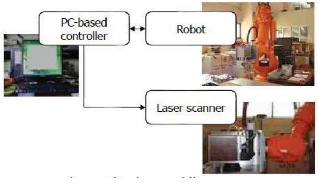
3.3
Working principles of RLW
RLW system normally integrates a commercial robotic arm, a 3D scanner, control
system and laser source. Figure 3. 3 illustrates a robot and a scanner that are
controlled by a PC-based controller. RLW can significantly reduce positioning time
by application of 3D scanner, which helps to increase the productivity of the system.
In addition, thanks to the long focal length and application of 3D scanner, RLW
system extends the stand-off distance from the workpiece and enables welding
evolved from merely two dimensions operation to three dimensions operation and
becomes able to weld more complicated parts in space than merely simple parts such
Figure 3. 3 An example of RLW system (adapted from (Kang et al., 2011))
Compared to conventional PLW, RLW is restricted to deliver process media like
gases or metal fillers to the welding interaction zone (Grupp et al., 2003). Shielding
gas could only be supplied independent of laser beam. One possibility is to integrate
the gas supply nozzles into the clamping devices. With numerous welding stitches,
the expenditure of this solution increases significantly. As shielding gases are usually
very expensive, compressed air is often alternatively chosen to eliminate the effects
of plasma (Grupp et al., 2003). (Grupp et al., 2003) also concluded when the system
power is under 3kW, conrresponding to power density of 1.5 * 106 W/cm2, the weld
depth (penetration) is not affected by the shielding gas. Figure 3. 4 summarizes the
above mentioned phenomenon. When power density is over 1.5 * 106 W/cm2, helium
Figure 3. 4 Plasma shielding at high laser power [0.5, 6] kW; speed= 2m/min, mild steel, from Grupp et al., 2003
3.4
Conduction-limited vs Keyhole wleding
There are mainly two types of welding mechanism: conduction-limited welding
(Figure 3. 5) and keyhole welding (Figure 3. 6). The former occurs when the power
density is insufficient to boil the material in the weld pool. The latter provides
sufficient energy per unit length to create vaporization in the weld pool and in
consequence a stable hole occurs. The keyhole behaves like an optical black body in
which the radiation enters and it is subjected to multiple reflections, as a result high
Figure 3. 5 Conduction welding mode, from (Steen and Mazumder, 2010)
3.5
Zinc degassing solutions
In the occasion of laser welding galvanized steel, as described previously, due to the
characteristic that the boiling temperature of zinc (906 °C) is much lower than the
melting temperature of steel (1530 °C), zinc has already turned into vapour while
steel is being heated up. There is high risk of expulsion of the weld metal (spatter)
and considerable surface porosity and entrapped porosity in the weld joint if the gap
is insufficient for the zinc vapour to exhaust (Zhao et al., 2012, Sinha et al., 2013,
Bley et al., 2007, Chen et al., 2009, Fabbro et al., 2006, Schmidt et al., 2008,
Yih-fong, 2006). Another problem induced by this zinc coating described by (Chen et al.,
2009) is that Zinc gives rise to strongly ionized plasma and it affects the absorption
and scattering of incident radiation and prevents the beam propagation through it,
which results in penetration reduction, as well as seam discontinuity and seam
narrowing.
A great many studies have discussed this problem and proposed solutions. U.S.
Patent 3969604 proposed a way of adding additional elements to the surface which
form a compound with the vaporized zinc (Baardsen, 1975). U.S. Patent 4642446
recommended to remove the zinc coating in the welding area and to replace it with a
metal with higher boiling point like nickel (Pennington, 1987). U.S. Patent 4691093
used a dual focus beam to elongate the keyhole (Banas and Doyle, 1987). U.S. Patent
6740845 used oscillated laser beam along or transverse the weld seam (Stol and
In summary, the solutions could be mainly classified into three directions. One
direction focused on creating clearance, another one focused on adjusting laser beam,
and the other one concentrated on changing the property of zinc.
Auto industry’s favourite solution is the creation of a gap between the to-be-welded
sheets. Nowadays, in automotive industry, usually shims (difficult to control the
consistency) or dimples (more realistic and under further investigation) are used to
obtain an appropriate gap. (Steen and Mazumder, 2010) claimed the calculation of
the gap size by physical and mathematical deduction. Equation 3. 1 is the theoretical
conclusion. Figure 3. 7 is the schematic picture of laser welding zinc-coated steel
with a small gap between the sheets for exhausting of the high-pressure zinc vapour.
The conclusion of this study is that when the gap is less than 40% of upper thickness,
it is possible to produce sound weld free from defects such as spatters and pitting.
g: part –to-part gap
t: upper sheet thickness
k: a constant related to material properties
V: welding speed
B: a constant related to material properties, for galvanized mild steel B=1
β: coefficient of thermal expansion
[image:57.595.177.486.274.676.2]Figure 3. 8 Operational diagram for the welding of zinc-coated mild steel with a gap for zinc vapour exhaust (excerpted from Steen and Mazumder (2010))
In this study, the direction of creating an appropriate gap is chosen to avoid zinc
vaporization. A fixture is specially designed to control the accuracy and consistency
the gap to ensure the research quality.
3.6
Process modelling and optimization
(Benyounis and Olabi, 2008) wrote a comprehensive reference guide about
Design of experiments (DoE), evolutionary algorithms and computational network
are widely used to develop mathematical relationship between the welding process
input parameters and the output variables of the weld joint in order to determine the
welding input parameters that lead to the desired weld quality (Benyounis and Olabi,
2008).
A comprehensive literature review of application of these methods in laser welding
will be classified according to methodologies used to develop aforementioned
correlations, i.e. Response Surface Methodology (RSM), Artificial Neural Network
(ANN), Taguchi methods and other techniques.
RSM
(Benyounis et al., 2005b) has constructed empirical models using response surface
methodology to predict heat input, penetration, welded zone width and heat affected
zone width under differing laser power, welding speed and focal point position. A
continuous 1.5 kW CO2 laser was used to butt weld medium carbon steel.
Box-Behnken design with full replicates was favoured as the experimental designing
strategy. This investigation came to the conclusions that Box-Ben design worked
well and the models developed could predict well which was demonstrated by
confirmation experiments. Furthermore, welding speed has a negative effect on all
the responses, whereas the laser power has positive effect. With the focused point
thick AISI 304 stainless steel plate. Central Composite Design (CCD) was chosen to
identify the trials. Beam power, welding speed and beam angle were related to depth
of penetration, bead width and area of penetration. This investigation shows CCD is
an easy tool to be used to analyse the process parameters on response. Beam power
has a positive effect on all the response variables however beam angle and welding
speed vice versa. Furthermore, it is also found there is small variation in weld width,
which enlightens that weld width is not much affected by the input variables.
(Padmanaban and Balasubramanian, 2010) studied the influence of laser power,
welding speed and focal position on the tensile strength of AZ31B magnesium alloy
after being welded by a CO2 laser in butt welding configuration. Thirty-three central
composite face centred design with full replicates was selected. The results indicate
the welding speed has the greatest influence on the tensile strength, followed by laser
power and focal position. In addition, maximum tensile strength is obtained under
The regression models could be a valuable starting point to develop a closed loop
control of the responses within process window. Laser power was found to be the
most influential variable. When the power is increased or welding speed is lowered,
the penetration and melted area increase, on the contrary, the plasma temperature
goes the opposite direction.
(Khan et al., 2011) related welding parameters (i.e. laser power, welding speed and
focal position ) to each of the weld characteristics (i.e. weld width, weld penetration
depth, resistance length and shearing force) of a lap joint configuration of martensitic
AISI 440FSe and AISI 416 stainless steels. The laser used is a CW 1.5 kW Nd:YAG.
Full factorial design was applied in this study. Numerical and graphical methods are
both applied to optimize the process based on the models obtained by RSM. Laser
power and welding speed are concluded to be the most important factors affecting
the weld bead geometry as well as shearing force. Fibre diameter has little effect on
weld bead profile and shearing force. However, its interactions with others affect a
great deal. Graphical optimization results were claimed to be quicker search of
optimum. Strong and efficient weld joints could be obtained using the parameters
from numerical optimization algorithm.
(Zhao et al., 2012) worked on rather thin-gauge galvanized steel with thickness of
0.4 mm in a lap joint configuration. They studies the effects laser power, speed, gap
and defocus could bring to the weld width, weld penetration and concavity of the
and total area) in the configuration of pulsed Nd:YAG laser welding of Al-alloy 5754.
Neural network was chosen as the modelling methodology. The controllable
parameters were travel speed, average power, pulse energy and pulse duration. They
developed a routine to convert the shape parameters into a predicted weld profile
which was based on the actual experimental weld profile data. This approach to
predicting weld pool shapes allows for an instantaneous prediction of weld pool
shape and therefore offers advantages in application where real-time predictions are
needed and computationally intensive predictions are too slow.
(Jeng et al., 2000) have used both back propagation (BP) and learning vector
quantization (LVQ) networks to relate work piece thickness, welding gap, power,
speed and focal position to weld width, undercut and weld distortion in a butt joint
configuration. Both these two techniques were proved to be successful in making
predictions. The models are quite useful in selecting suitable welding parameters and
Taguchi method
(Pan et al., 2005) studies the effect of Nd:YAG laser welding parameters (shielding
gas type, laser energy, conveying speed, laser focus, pulse frequency and pulse shape)
on the ultimate tensile strength of butt-welded thin plates of magnesium alloy using
Taguchi method. The analytical results indicate that the pulse shape and the energy
of the laser contributed the most. Accordingly, the optimal combination of welding
parameters for this process is Argon as the shielding gas, a 360 W laser, a work piece
speed of 25 mm/s, a laser focus distance of 0.0 mm, a pulse frequency of 160 Hz, and
a type 3 pulse shape. The ultimate tension stress was at maximum an overlap of the
welding zone of approximately 75%.
The purpose of the study by (Lee et al., 2006) is to optimize Nd:YAG laser welding
parameters to seal an iodine-125 radioisotope seed into a titanium capsule. The
accurate control of the melted length of the tube end was affected by the laser
welding parameters (nozzle type, rotating speed, tilt angle, focal position, pumping
voltage, pulse frequency, and pulse width). After being analysed and optimized by
Taguchi and regression analysis method, it was found that the laser pulse width and
focal position among the welding parameters had the greatest effects on the melted
length. Optimal welding conditions were obtained through this study, and
confirmation experiments validated this result very well.
stainless steel) dissimilar lap welding joints under CO2 laser welding using analysis
of variation (ANOVA) and signal-to-noise ratio method. Laser power, welding speed,
and focused position were considered as the main factors of the process. 3 factors, 5
levels L-25 orthogonal array was used as the strategy of designed experiments. Joint
strength was determined using the notched-tensile strength method. Conclusions
were made as following: laser power is the main factor affecting the process; the
speed also has a strong negative effect on the response; however, focus position had
no obvious effect on the tensile strength. The welding joints have better mechanical
properties compared to the base metals. Furthermore, the models can predict
adequately within the factors domain and optimal working conditions were obtained
and confirmed through confirmation tests.
(Sathiya et al., 2011) have studied the correlation between input variables (i.e.
shielding gases (argon, helium and nitrogen), beam power, travelling speed and focus
position) and tensile strength and bead profiles (bead width and depth of penetration)
variables simultaneously. Both analyses are proved to be accurate techniques to
optimize the laser welding process.
Comparisons among the optimization techniques
According to (Benyounis and Olabi, 2008), RSM performs better than other
techniques, especially ANN and GA, when a large number of experiments are not
affordable. The trend in the modelling using RSM has a low order non-linear
behaviour with a regular experimental domain and relatively small factors region,
due to its limitation in building a model to fit the data over an irregular experimental
region. Moreover, the main advantage of RSM is its ability to exhibit the factor
contributions from the coefficients in the regression model. This ability is powerful
in identifying the insignificant quadratic terms in the model and thereby can reduce
the complexity of the problem. This technique required good definition of ranges for
each factor to ensure that the response under consideration is changing in a regular
manner within this range. The most popular designs within RSM designs are the
central composite design (CCD) and Box-Behnken design (BBD). In regard to ANNs,
it noted that ANNs perform better than other techniques, especially RSM when
highly non-linear behaviour is the case. Also, this technique can build an efficient
model using a small number of experiments; however the technique accuracy would
be better when a larger number of experiments of experiments are used to develop a
model. The ANN model itself provides little information about the design factors and
RSM is chosen as the ideal modelling algorithm and BBD experimental design is
sufficient for this purpose. and methods used.
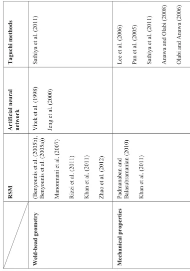
Table 3. 1 represents comparisons among those common modelling/optimizing
techniques for laser welding. Table 3. 2 classifies all the aforementioned works into
several groups based on different methods used and various characteristics of interest.
Table 3. 3 provides detailed information about laser sources, material types, process
parameters of interest, performance characteristics of interest, and methods used.
Table 3. 1 Comparison among the common modelling/optimizing techniques for laser welding (adapted fromBenyounis and Olabi (2008))
Optimization Through model Through model Straight
Understanding Easy Moderate Normal
Availability in software
Available Available Available
Optimization accuracy level
Very high High Normal
Ya
n
g
[image:68.595.94.475.130.672.2]lin Shi (
Table 3. 2 Sum
m
a
ry of
all the me
ntioned studies of
m
o
delling and o
p ti m izing f RSM Ar tificial neural network -bead geome tr y (B en y ounis
et al. (2005b)
, B en y ounis et al. (2005 a))
Manonmani et al. (2007) Rizzi et al. (2011) Kha
n et al. (2011
)
Z
h
ao
et al. (2012)
Vitek e
t al. (1998)
Je
ng
et al. (2000)
Padmana
ban and
B
alasubramanian (2010)
Kha
n et al. (2011
f Warwick
Ya
n
g
[image:69.595.96.501.57.735.2]lin Shi (
Table 3. 3 Sum
m a ry of detailed inf o rm ation of the st
udies for m
o
delling and op
tim izing of lase r w e lding L as er t y pe Materials
Weld config
u ra tion Input va riables Output variables Methods CW 2 kW
solid state Nd:YAG laser 2.5 mm austenitic stainless steel 304 sheet
B
utt joint
L
as
er beam power
[580, 750, 1000, 1250, 1420] Welding
spee
d
[580,750, 1000, 1250, 1420] Incident an
g
le
[
82,
85,90,95, 98] (Shielding
g
as
constant)
Penetration depth Bead width Penetration ar
ea RSM (CCD) al. CW 1.5 kW CO 2 laser
Medium carbon steel
B
utt joint
L
as
er power
[1200,1312, 1430 ] Weld speed
[
300,
500, 700] Fo
cal point position
[-2.5, -1.25, 0]
Penetration Weld z
Ya
n
g
lin Shi (
CW 2.5 kW CO 2 laser Stainless steel L ap joint L as er power [ 900,
1200, 1500] Welding
spee
d
[2400, 3000, 3600]
CW CO 2 laser AZ 31 B mag n esium all o y B utt joint L as er power
[2500,3000, 3500] Welding
spee
d
[4500, 5000, 5500] Fo
cal position [ 0,-1.5, -3] CW1.5 kW Nd:YAG laser Mar tensitic A IS I 440 F S e and A IS I 416 stainless steels L ap joint L as er power [ 800,
950, 1100] Welding
spee
d
[4500,6000,7500] Fiber diamet
f Warwick
Ya
n
g
lin Shi (
laser
SAE1004 steel
Welding
speed
[180, 210, 240] Pre
scribed g
ap
[
0.1,
0.15, 0.2] De
foc
us amount
[0,
-0.1,
-0.2]
Weld width Concave
A
utog
en
ous
pulsed Nd:YAG laser
3
mm
Aluminium allo
y 5754 2mm allo y 6111 Plate test Ave rage power
Weld speed Pulse ener
g
y
Pulse duration
Pe
netration
depth Top surfa
ce width Ha lf -width Ex perimental we ld profile ANN B utt joint Work piec e thickness Powe r S p eed F o cal position
Weld distortion Weld width underc
ut
Ya
n
g
lin Shi (
f Warwick
Ya
n
g
lin Shi (
3.5
kW
cooled
slab lase
r
Austenitic stainless steel AIS
I 904 SASS
B utt joint B eam po we r Travellin g spee d F o cal position
Shielding gas
(Ar g on, Nitrog en, He lium) B ead width De pth of
penetration Tensile stren
g th Tag u chi method (3
3 full fa
ctorial desig n) Olabi 1.5 kW CO 2 las er F er ritic (middle
carbon mild steel) to austenitic(A
IS
I
316 stainless steel)
L
ap joint
L
as
er power
Weld speed Fo
cal position Notched -tensile streng th Tag u chi method (L -25 orthog on al arra y ) a 1.5 kW CO 2 laser F er ritic(middle
carbon mild steel) to austenitic(A
IS
I
316 stainless steel)
L
ap joint
L
as
er power
Weld speed Fo
quality, least welding time and power consumption. Table 4. 1 lists out all the
stack-ups of interest. The roadmap of achieving the goals is proposed in the following
paragraph.
4.1
Problem-solving roadmap
Materials are welded in the configuration of lap joint. It could be seen that the four
stack-ups share the same upper material but lower materials are different. According
to EN10327 2004.6, the materials with different designations have same chemical
composition but slightly different mechanical property. The significant difference
among them is the lower thickness.
Table 4. 1 Stack-ups of case study
Stack-up
Upper material designation
Upper thickness
Lower material
designation
SU4 DX56D+Z 0.75 mm DX53D+Z 0.70 mm
Figure 4. 1 illustrates the roadmap of achieving the goals. Firstly factors affecting the
RLW process in the circumstance of welding galvanized steel are identified. In this
step, fishbone diagram is used to analyse all potential factors systematically. After
the factors of interest are selected, process window within which weld joints
fulfilling all requirements could be produced is preliminarily specified using
One-Factor-at-a-Time method. In the third step, statistical comparison analysis between
SU2 and SU3 is carried out to check whether the lower thickness is significantly
affecting the process. The assumption is if the influence is insignificant and
negligible, modelling for four stack-ups could be simplified to only the stack-up with
thickest lower material assuming the other three stack-ups share the model. In this
case, the overall number of experiments could be significantly reduced. Otherwise,
experimentation campaign needs to be repeated four times. Finally, optimization is
4.2
Identification of process factors
The process of laser welding galvanized steel is quite complicated with numerous
factors affecting the outcomes. The controllable factors of interest should be
identified and analysed how they are influencing the output, while the uncontrollable
ones shall be kept as constants. (Steen and Mazumder, 2010) proposed all the factors
[image:77.595.149.541.274.620.2]that should be considered for a laser welding process are listed in Figure 4. 2.
¾ Power: this is a controllable factor of interest
¾ Laser mode: Continuous Wave
Other process parameters
¾ Gap: this is a controllable factor of interest
¾ Incident angle: programmed to be perpendicular to the surface, but how the
programming is done is not clear.
¾ Speed: this is a controllable factor of interest
¾ Material thickness: as listed in Table 4. 1
¾ Material compositions: further investigated in Chapter 5
¾ Environment: Warwick manufacturing centre, autumn, room temperature, no
specific control of humidity
4.3
Methodology for process window identification
The factors to be further investigated are weld speed, power, and gap. The process
window is screened based on the criteria that all weld joints are soundly welded free
from visible defects such as spatter, cracks, cut-through and burn-through. The
ranges of factors are preliminarily set as in Table 4. 2. According to TSB project, in
the following ranges, all different welding behaviours could be covered, including
[image:79.595.112.529.410.661.2]sound weld, pitting, spatter, insufficient weld and etc.
Table 4. 2 Ranges of process factors
Factor Type Range Unit
Speed Variable [1:12] m/min
Power Variable [2:4] kW
Gap Variable [0.05:0.5] mm
Weld in a big range
Sound weld?
Cross-section the sound
welds
Fulfill the weld
bead profile ?
Decide process window
Yes
Yes
Criterion:
Free from visible defects
(spatter, top surface cracks,
cut-through, burn-cut-through, weld
discontinuity etc.)
Criterion:
Penetration≥
0.3×lower thickness
Interface width≥
0.9×thinner thickness
Top
concavity≤
0.5×upper thickness
Bottom
concavity≤
0.5×lower thickness
Ɋଶ. If it is assumed that ୢ ൌ Ɋଵെ Ɋଶ, then the equivalent testing hypothesis is
ǣୢ ൌ Ͳ
ǣୢ ് Ͳ
The test statistic for the above hypothesis should be:
ൌ ത
ୢȀξ
where ത ൌଵ
୬σ ୨ ୬
୨ୀଵ is the sample mean of the differences between pairs and n is the
sample number.
ୢ ൌ
σౠసభሺୢౠିୢഥሻమ
୬ିଵ ൨
ଶ
is the sample deviation of the paired differences.
In this test, if ଶ
4.5
Response surface methodology
Experimental Design
Box-Behnken Design (BBD) is chosen as the experimental design of this study. It is
an efficient three-level design for fitting second order models based on balanced
incomplete block designs, first developed by Box and Behnken in 1950. To illustrate
the basic idea of BBD, let us assume the total number of process parameters is k. In
BBD, factors are paired together, that is, in total k*(k-1)/2 pairs. Each pair is lined
with a 22 factorial design, while the (k-2) factors remain in the centre. If the number
of runs with all the process parameters in centre is denoted as nc, then the total run of
a BBD design with k parameters is 2k*(k-1)+nc. For instance, if k=3, then at least
12+nc runs are needed. In Figure 4. 4, it graphically show the scattering structure of
three factors three levels BBD. Usually in a BBD, in order to be efficient and reduce
the number of trials, only the centre points are replicated for several times.
Replicated centre points are very crucial for pure error and lack-of-fit analysis. When
BBD is applied, it is assumed phase zero of factor screening and phase one of
steepest ascent/descent with factorial design have been conducted and the region of
ൌ Ⱦ Ⱦଵଵ Ⱦଶଶ ڮ Ⱦ୩୩ ɂ
This model is called multiple linear regression model with k parameters, the Ⱦ୨ǡ ൌ
Ͳǡͳǡ ǥ ǡ , are called regression coefficients.
However, sometimes the correlation could be much more complex. Thus
second-order polynomial is chosen as a very good model to depict non-linear relationships.
The second-order response surface with k=2process parameters, could be denoted as
the following equation:
ൌ Ⱦ Ⱦଵଵ Ⱦଶଶ Ⱦଵଵଵଶ Ⱦଶଶଶଶ Ⱦଵଶଵଶ ɂ
Seemingly the second-order model is different from the first order on and could be
much hard to deal with and calculate the coefficient. However, if we let ଷ ൌ
ଵଶǡ ସ ൌ ଶଶǡ ହ ൌ ଵଶǡ Ⱦଷ ൌ Ⱦଵଵǡ Ⱦସ ൌ ȾଶଶȾହ ൌ Ⱦଵଶ, then the model could be
of the errors between the observations and the predictions by the model. The
observations could be denoted as
୧ ൌ Ⱦ Ⱦ୨
୩
୨ୀଵ
୧୨ ɂ୧ǡ ൌ ͳǡʹǡ ǥ
Then the least squares function is
ൌ ɂ୧ଶ
୬
୧ୀଵ
ൌ σ୬୧ୀଵሺ୧െ Ⱦെ σ୩୨ୀଵȾ୨୧୨ሻଶ
The objective is to find a set ofȾ’s that minimizes the L function. Mathematically to
do so, the first derivative of the equation should be equal to zero at the same time
with the set ofȾ’s. That is,
μ
μȾȁୠబǡୠభǡǥǡୠౡ ൌ െʹ ሺ୧െ െ ୨୧୨
୩ ୨ୀଵ ሻ ୬ ୧ୀଵ ൌ Ͳ and μ μȾ
ȁୠబǡୠభǡǥǡୠౡ ൌ െʹ ሺ୧െ െ ୨୧୨
୩
୨ୀଵ
ሻ
୬
୧ୀଵ
୧୨ ൌ Ͳ

![Figure 3. 4 Plasma shielding at high laser power [0.5, 6] kW; speed= 2m/min, mild steel, from Grupp et al., 2003](https://thumb-us.123doks.com/thumbv2/123dok_us/9496306.455296/53.595.141.493.71.313/figure-plasma-shielding-laser-power-speed-steel-grupp.webp)