warwick.ac.uk/lib-publications
Original citation:
[Barp, Alessandro, Barp, Edoardo Gabriele, Briol, François-Xavier and Ueltschi, Daniel. (2015)
A numerical study of the 3D random interchange and random loop models. Journal of
Physics A: Mathematical and Theoretical, 48 (34). 345002.
Permanent WRAP URL:
http://wrap.warwick.ac.uk/
7
5301
Copyright and reuse:
The Warwick Research Archive Portal (WRAP) makes this work by researchers of the
University of Warwick available open access under the following conditions. Copyright ©
and all moral rights to the version of the paper presented here belong to the individual
author(s) and/or other copyright owners. To the extent reasonable and practicable the
material made available in WRAP has been checked for eligibility before being made
available.
Copies of full items can be used for personal research or study, educational, or not-for-profit
purposes without prior permission or charge. Provided that the authors, title and full
bibliographic details are credited, a hyperlink and/or URL is given for the original metadata
page and the content is not changed in any way.
A note on versions:
The version presented here may differ from the published version or, version of record, if
you wish to cite this item you are advised to consult the publisher’s version. Please see the
‘permanent WRAP URL’ above for details on accessing the published version and note that
access may require a subscription.
RANDOM LOOP MODELS
ALESSANDRO BARP, EDOARDO GABRIELE BARP, FRANC¸ OIS-XAVIER BRIOL, AND DANIEL UELTSCHI
Abstract. We have studied numerically the random interchange model and related loop models on the three-dimensional cubic lattice. We have determined the transition time for the occurrence of long loops. The joint distribution of the lengths of long loops is Poisson-Dirichlet with parameter 1 or 12.
1. Introduction
The random interchange model is a stochastic process where transpositions are selected at random. The product of these transpositions gives a random permutation and the main question deals with its cycle structure. We consider variants where possible transpositions are restricted to nearest-neighbours of a regular cubic lattice. We also consider related loop models where “crosses” are replaced by “double bars”. We provide evidence that a phase transition takes place where macroscopic loops occur. We give good estimates of the values of the parameters at the transition point, which should help to better comprehend the model. Finally, we compute moments of the lengths of the loops; it turns out that they are identical to those of the Poisson-Dirichlet distribution.
The random interchange model was invented by Harris [11]; T´oth used it as a represen-tation of the spin 12 quantum Heisenberg ferromagnet [16]. Angel [3] and Hammond [10] obtained results for the model on trees. Schramm considered the variant on the complete graph and he proved that the joint distribution of the large cycle lengths is Poisson-Dirichlet of parameter 1, following a conjecture of Aldous [15]; see also [4] for some simplifications and extensions. Alon and Kozma have obtained remarkable identities that give the probability of cyclic permutations in terms of eigenvalues of the graph Laplacian, for arbitrary graphs [2]. These have allowed Berestycki and Kozma to obtain further results on the complete graph [5].
A similar model with “double bars” instead of “crosses” was introduced by Aizenman and Nachtergaele in order to describe the spin 1
2 quantum Heisenberg model and the spin
1 model with biquadratic interactions [1]. It should be noticed that the representation of quantum systems involves the extra factor θ#loops with θ = 2,3... In the survey [8], the
authors conjectured that the joint distribution of the lengths of long loops, in dimensions three and higher, is given by the Poisson-Dirichlet distribution of parameterθ. The two representations of T´oth and Aizenman-Nachtergaele were recently combined so as to describe quantum models that interpolate between the two Heisenberg models, such as the spin 12
1991Mathematics Subject Classification. 60K35, 82B20, 82B26.
Key words and phrases. Random interchange model; random loop model; macroscopic loops; Poisson-Dirichlet distribution.
Work partially supported by a URSS grant from the University of Warwick. c
2015 by the authors. This paper may be reproduced, in its entirety, for non-commercial purposes. 1
quantum XY model and further spin 1 models with SU(2)-invariant interactions [18]. For these models, the joint distribution of long loops should be Poisson-Dirichlet with parameter
θ/2. The consequences of this structure have yet to be worked out. One such consequence is to identify the nature of symmetry breaking in the spin 1 model [19].
The Poisson-Dirichlet distribution is conjectured to be a common feature of “loop soups” in dimensions three and higher. This was confirmed numerically in lattice permutations [9] and in O(N) loop models [13]. This was also confirmed, with a mathematically rigorous proof, in an annealed model of spatial permutations [6]. A numerical study of the spin 1 model [20] also provides indirect evidence, as explained in [19]. However, this conjecture is far from being accepted nowadays. It thus seems necessary to verify it also in those loop models that are related to quantum spin systems.
We introduce the random loop models in Section 2.1. The conjectures about the joint distribution of the lengths of long loops are explained in Section 2.2. Numerical evidence is presented in Section 3 for the occurrence of a phase transition; we also discuss a comparison with bond percolation and quantum Heisenberg models. We investigate the presence of the Poisson-Dirichlet distribution in Section 4.
2. Random loop models
2.1. Definitions. Let Λ ={1, . . . , N}3 ⊂
Z3, and let EΛ denote the set of edges
(nearest-neighbours) in Λ. Letβ >0 andu∈[0,1]. To each edge ofEΛis associated an independent
Poisson point process on the interval [0, β] with two kinds of events:
• crosses occur with intensityu;
• double bars occur with intensity 1−u.
β
Λ
β
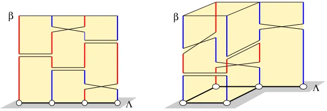
[image:3.612.152.475.412.522.2]Λ
Figure 1. Graphs and realisations of Poisson point processes, and their loops. In both cases, there are exactly two loops.
See Fig. 1 for an illustration. Given a realisationω, we define loops by moving in the vertical direction, and by jumping to the neighbour whenever a cross or a double bar is encountered. If it is a cross, one continues in the same vertical direction; if it is a double bar, one continues in the opposite vertical direction. We assume periodic boundary conditions in the vertical direction. All trajectories must close, resulting in loops. We use the following notation for the relevant random variables.
• L1(ω), L2(ω), . . . denote the vertical lengths of all the loops in decreasing order
(repeated with multiplicities); notice that 0< Lj(ω)≤β|Λ|for allj.
• `1(ω), `2(ω), . . . denote the “shadow lengths” of the loops in decreasing order
Notice that for all realisationsω, we haveP
j≥1Lj(ω) = β|Λ| and Pj≥1`j(ω) =|Λ|. The following are random partitions of [0,1]:
L 1(ω)
β|Λ| ,
L2(ω)
β|Λ| , . . .
,
` 1(ω)
|Λ| ,
`2(ω)
|Λ| , . . .
. (2.1)
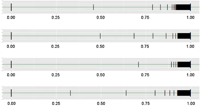
When β is small, crosses and double bars are scarce and loops are small. But a phase transition occurs asβ grows and some loops become macroscopic. A few random partitions are displayed in Fig. 2; they were measured in a cube of volume 1603, for a value ofβ that
[image:4.612.138.464.242.417.2]is above the critical parameter. Occurrence of macroscopic loops is manifest.
Figure 2. Samples of random partitions observed in a cube of sizeL= 160, for u = 1 and β = 1. Notice that m(β) appears to be constant with approximate value 0.9.
2.2. Phase transition and universal behaviour. The patterns of the random partitions suggest a very interesting strong law of large numbers. It is worth describing in details, since it is expected to occur in all models of “loop soups”.
Conjecture 1. There existsm(β)such that, asL→ ∞, we have for almost all realisations ω:
lim K→∞Llim→∞
K
X
j=1
`j(ω)
|Λ| =m(β),
lim k→∞Llim→∞
X
j:`j≤k
`j(ω)
|Λ| = 1−m(β).
(2.2)
The functionm(β) represents the mass of points in long loops. It is equal to 0 whenβ is small, and it becomes positive whenβ crosses the transition point. Eq. (2.2) says that loops are either microscopic (the length is of order 1) or macroscopic (the length is of order|Λ|); the number of sites that belong to loops of intermediate, mesoscopic length, has vanishing density.
The next conjecture is about the joint distribution of the lengths of the macroscopic loops, which should be Poisson-Dirichlet (PD). Let us recall the closely related Griffiths-Engen-McCloskey (GEM) distribution and its “stick breaking” construction. LetX1, X2, . . .
be i.i.d. Beta(1,ϑ) random variables; their probability density function is ϑ(1−s)ϑ−1 for
0≤s≤1. The following is a random sequence with GEM(ϑ) distribution:
X1,(1−X1)X2,(1−X1)(1−X2)X3, . . .. (2.3)
It is not hard to verify that the sum of all these numbers is 1 with probability 1. Rearranging the numbers in decreasing order, we get a random partition with PD[0,1](ϑ) distribution.
Multiplying each element bym, the distribution is PD[0,m](ϑ). We can formulate the
con-jecture about the joint distribution of macroscopic loops.
Conjecture 2. For any k, the joint distribution of`1, . . . , `k converges to the joint
distri-bution of the firstk elements of a random partition with PD[0,m(β)](ϑ)distribution, where
ϑ=
(
1 ifu= 0 or1;
1
2 ifu∈(0,1).
Here,m(β) is the same quantity as in Conjecture 1. In random loop models with weights
θ#loops, the conjecture holds withϑ=θ ifu= 0,1, andϑ=θ/2 if u∈(0,1).
The heuristics for this conjecture goes back to Aldous’ ideas for the complete graph, which Schramm eventually managed to turn into a proof [15]. Its relevance for models with spatial structure was suggested in [8, 9]. In summary, the idea is to consider the stochastic process restricted on random partitions. Adding crosses or double bars result in splits or merges of elements of the partition. The rate at which two long loops merge may seem at first sight to depend on the exact geometry of the loops, which is very intricate. But averages take place when the loops are macroscopic, which is the case in dimension 3 and higher. The effective stochastic process is then a standard split-merge process, whose invariant measure is Poisson-Dirichlet.
The addition of a transition (cross or double bar) between different loops always results in a merge. Whenu= 1, or whenu= 0 on a bipartite graph, the addition of a transition within the same loop always results in a split. It follows that the Poisson-Dirichlet distribution has parameterϑ= 1. When 0< u <1, the addition of a transition within the same loop may split it, or it may rewire it. The splits occur therefore at half the rate of the merges, and the Poisson-Dirichlet distribution has parameterϑ= 12. See [8, 9, 13, 18] for more detailed explanations.
3. Phase transition and critical parameters
3.1. Fraction of sites in long loops. We seek a convenient expression for the mass of sites in macroscopic loops m(β). The expressions of Conjecture 1 turn out to be inconvenient and we use Conjecture 2 instead. It allows to relatem(β) with the moments of the lengths of the loops, see Eq. (3.4) below. We now give a derivation of this result.
We start with
E
X
j≥1 `j
|Λ|
2
= 1
|Λ|2 X
j≥1
E
X
x,y∈Λ
1(x,0)∈jth loop1(y,0)∈jth loop
= 1
|Λ|2 X
x,y∈Λ
P (x,0)↔(y,0).
If we accept Conjecture 2, the probability that two sitesx, y, that are far apart, belong to the same loop, is given by the probability that they both belong to long loops — this is equal to m(β)2 — times the probability that two random numbers in [0,1] belong to the same element in the partition. The latter probability can be calculated using the GEM random sequence (2.3). The probability that both random numbers belong to thejth element is
Z 1
0
ds1 Z 1
0
ds2EGEM(ϑ) 1s1,s2∈jth element
=EGEM(ϑ)(Yj2)
=EBeta(1,ϑ) (1−X)2 j−1
EBeta(1,ϑ) X2
.
(3.2)
Elementary computations giveEBeta(1,ϑ) (1−X)2
= ϑ+2ϑ andEBeta(1,ϑ) X2
=(ϑ+1)(2ϑ+2). The probability that two distant sites belong to the same loop is therefore approximately equal to
P (x,0)↔(y,0)=m(β)2
X
j≥1
ϑ
ϑ+ 2
j−1 2
(ϑ+ 1)(ϑ+ 2) =
m(β)2
ϑ+ 1. (3.3)
Using (3.1), we obtain an expression that is convenient for numerical calculations, namely
m(β) =
s
(ϑ+ 1)EX j≥1
`j
|Λ|
2
. (3.4)
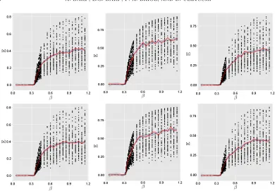
Our numerical results are displayed in Fig. 3. As expected,m(β) is zero for small β and positive forβ large enough. m(β) is also continuous and increasing. Notice also that, when
u= 1, it converges to 1 asβ → ∞; indeed, all sites belong to long loops. It converges to a value smaller than 1 whenu= 0 or 12 because a density of small loops remains present in the system.
3.2. Value of the critical parameter βc(u). The previous results confirm the existence
of a phase wherem(β) is positive. We define the critical parameter by
βc(u) = inf{β:m(β)>0}. (3.5)
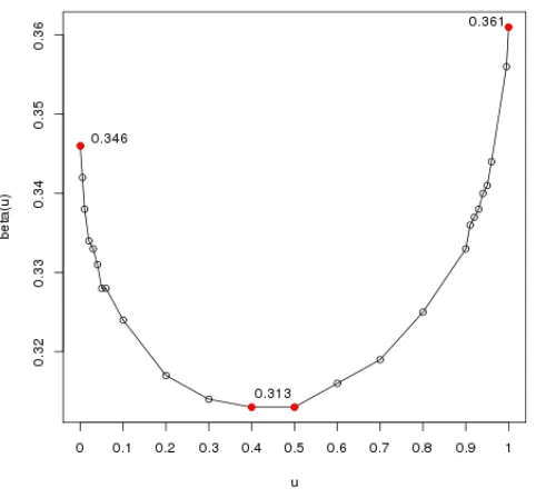
It is instructive to estimate its value and to investigate its dependence on the parameteru. Our numerical results are depicted in Fig. 4. We find thatβc(u) is a convex function ofu.
Its minimal value occurs whenuis close to 0.5. The derivative of βc(u) diverges atu= 0
andu= 1. In retrospect, this is perhaps not surprising: The model with weight 2#loopshas more symmetry atu= 0 andu= 1, SU(2) rather than U(1), so that a minor change in the value ofuhas major consequences. This also explains whyβc(12)< βc(0) andβc(12)< βc(1):
Less symmetry means reduced fluctuations so that spontaneous magnetisation occurs more easily in systems with U(1) symmetry rather than SU(2). Somehow, this explanation should retain validity when the weight 2#loopsis not present.
3.3. Comparison with bond percolation, Ising, and quantum Heisenberg models. There are natural comparisons between the critical parameters of the model of random loops, of the Ising model (a.k.a. theq= 2 random cluster model), and the quantum ferromagnetic and antiferromagnetic Heisenberg models.
A. Bond percolation. Given a realisationωof crosses and double bars onEΛ×[0, β], there
Figure 3. Numerical values forE Pj≥1
`j |Λ|
2
as function ofβ. The size of the cube isL= 80 in the top row andL= 160 in the bottom row. The parameteru takes values 0 (left), 0.5 (centre), and 1 (right). The points represent the values ofP
j( `j |Λ|)
2 for many realisations; the curve gives the
average.
loopγ∈ L(ω) is contained in some cluster C∈ C(ω) in the sense thatγ⊂C×[0, β]. Then
|C(ω)| ≤ |L(ω)|and the presence of long loops is possible only when percolation occurs. The critical parameter for the cubic lattice ispc= 0.2488, which gives βcper=−log(1−
pc) = 0.286. We have indeed found thatβc(u)> βcper for allu∈[0,1], and the inequality is
strict.
B. Random cluster and Ising model. The random cluster model is similar to bond percolation, but with configurations η receiving the extra weight q|C(ω)|. The random cluster model is closely related to the q state Potts model; their transition parameters satisfy prc.c.(q) = 1− e−β
Potts(q)
c . The case q = 2 is equivalent to the Ising model with 2βIsing
c =β Potts (q)
c . See [7, Section 3.8] for an excellent introduction to this topic. The Curie
temperature for the three-dimensional Ising model isTc= 4.51, which allows to deduce that
βcr.c.(q=2)=β
Potts (q=2)
c = 0.443.
There is no natural comparison betweenβcr.c.(q=2)of the random cluster model, andβc(u)
of the random loop model. But it can be compared withβper c andβ
(2)
c , see (3.7).
C. Quantum Heisenberg models. LetS1, S2, S3denote the usual spin operators in
C2 that satisfy [S1, S2] = iS
Figure 4. Value of the critical parameterβc as function ofu.
that acts on the Hilbert space⊗x∈ΛC2:
HΛ=−2 X
{x,y}⊂Λ
kx−yk=1
Sx1Sy1+ (2u−1)S2xSy2+Sx3Sy3
. (3.6)
The case u= 1 corresponds to the spin 12 Heisenberg ferromagnet; the case u= 12 is the quantum XY model; the caseu= 0 is unitarily equivalent to the Heisenberg antiferromagnet, provided Λ is bipartite.
The partition function and the quantum correlations can be expressed using random loop models where realisationsωreceive the extra weight 2|L(ω)|[16, 1, 18]. In particular,β(2)
c (u)
is equal to the inverse Curie temperature of the quantum model. Numerical studies have found thatβc(2)(1) = 0.59 [17] andβ
(2)
c (0) = 0.53 [14].
The extra weight encourages the system to have more, smaller loops, so we can expect
βc(2)(u)≥βc(u) for all u. Besides, we observe that β (2) c (0)< β
(2)
c (1), as in the absence of
the weight.
Regarding the quantum XY model, Stefan Wessel has just performed numerical calcu-lations and he obtained the valueTc = 1.008±0.001 for the Hamiltonian with interaction
−P
{x,y}(Sx1Sy1+Sx3Sy3) [21]. This implies thatβ
(2)
c (12)≈0.496. We conjecture thatβ (2) c (u)
has a shape similar to that ofβc(u).
Let us summarise the discussion above with the following inequalities; for all u∈[0,1],
βcper= 0.286≤
βc(u)∈[0.313,0.361]
βrc.c.(q=2)= 0.443
4. Joint distribution of the lengths of long loops
4.1. Calculation of the moments of Poisson-Dirichlet. We check the presence of the Poisson-Dirichlet distribution by looking at its moments, following [13]. Letn1≥ · · · ≥nk be integers. The calculation of the moments can be achieved by starting from another representation of the Poisson-Dirichlet distribution due to Kingman [12]. Let Z1, . . . , ZN be i.i.d. random variables with Gamma(Nϑ) distribution (that is, their probability density function issNϑ−1e−s/Γ(ϑ
N) for 0≤s <∞). LetS =Z1+· · ·+ZN. Consider the sequence
Z1
S , . . . , ZN
S
(4.1)
and reorder it in decreasing order, so it forms a random partition of [0,1]. AsN → ∞, this partition turns out to converge to PD[0,1](ϑ). The following two observations are keys to
our calculations:
• S is a Gamma(ϑ) random variable;
• S is independent of (Z1 S , . . . ,
ZN S ).
For given integersn1, . . . , nk≥0, using the independence ofS from the partition, we have
EPD[0,1](ϑ)
X
j1,...,jk≥1
distinct
Yn1 j1 . . . Y
nk jk = lim N→∞ N! (N−k)! E
Z1
S
n1
. . .Zk S
nk
= lim N→∞
N! (N−k)!
E Sn1+···+nk(Z1 S )
n1. . .(Zk S )
nk
E(Sn1+···+nk)
= lim N→∞
N! (N−k)!
Γ(ϑ)E Zn1
1 . . . Z
nk k
Γ(ϑ+n1+· · ·+nk)
.
(4.2)
We also usedE(Sa) = Γ(ϑ+a)/Γ(ϑ). Since theZ
is are independent,
E Z1n1. . . Z
nk k = k Y i=1
Γ(ϑ/N+ni)
Γ(ϑ/N) . (4.3)
Recall that Γ(ϑ/N)∼N/ϑasN → ∞, so that N!
(N−k)!Γ(ϑ/N)k →ϑ
k. We obtain
EPD[0,1](ϑ)
X
j1,...,jk≥1
distinct
Yn1 j1 . . . Y
nk jk
=ϑ
kΓ(ϑ) Γ(n
1). . .Γ(nk) Γ(ϑ+n1+· · ·+nk)
. (4.4)
This important formula appears in [13]. Its derivation there is different; it involves another loop soup model, assumes the presence of Poisson-Dirichlet, and uses a “supersymmetry” method.
Eq. (4.4) holds for Poisson-Dirichlet on the interval [0,1]. The formula for the interval [0, m] is identical, except for the additional factormn1+···+nk. Combining Conjecture 2 and Eq. (4.4), we get the following exact formula.
Conjecture 3. The moments of the lengths of the loops are given by
E
X
j1,...,jk≥1
distinct `j
1
|Λ|
n1
. . .`jk
|Λ|
nk
=m(β)n1+···+nkϑ
kΓ(ϑ) Γ(n
1). . .Γ(nk) Γ(ϑ+n1+· · ·+nk)
,
whereϑ= 1 foru= 0 oru= 1, andϑ=12 for0< u <1.
4.2. Numerical results. We now calculate numerically some moments of the joint distri-bution of the loops and compare the results with Conjecture 3. First, moments involving a single loop. Letmn1(β) be the value ofm(β) in Conjecture 3 whenn1 ∈Nandnj = 0 for
j≥2. Explicitly, we have
mn1(β) =
Γ(ϑ+n1)
ϑΓ(ϑ)Γ(n1)E X
j≥1 `j
|Λ|
n11/n1
. (4.5)
Our numerical results deal with β = 1, u ∈ {0,12,1}, and n1 ∈ {2,3,4,5} and they are
listed in Table 1. They show that mn1(β) is quite constant in n1, apart from numerical fluctuations and finite-size corrections. This confirms Conjecture 3. Notice that it confirms in particular thatϑis either 1 or 12, depending on the value ofu.
u
0 12 1
n1
[image:10.612.226.373.270.340.2]2 0.8925 0.9585 0.9310 3 0.8968 0.9587 0.9276 4 0.8815 0.9595 0.9217 5 0.8930 0.9528 0.9356
Table 1. Numerical values ofmn1(β) forβ = 1, andL= 160.
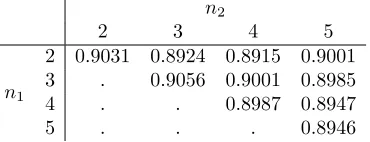
Next, let mn1,n2(β) be asmn1(β), but with n26= 0. The expression is
mn1,n2(β) =
Γ(ϑ+n 1+n2)
ϑ2Γ(ϑ)Γ(n
1)Γ(n2) E
X
j1,j2≥1
distinct `j
1
|Λ|
n1`j
2
|Λ|
n21/(n1+n2)
. (4.6)
The numerical values are listed in Tables 2–4 foru= 0,1
2,1. Notice that we avoid the values
ni = 1 because of undesirable effects due to small loops.
n2
2 3 4 5
n1
2 0.9031 0.8924 0.8915 0.9001 3 . 0.9056 0.9001 0.8985
4 . . 0.8987 0.8947
5 . . . 0.8946
Table 2. Numerical values ofmn1,n2(β) for u= 0, β = 1, and L= 160. Here, mL(β) = 0.872.
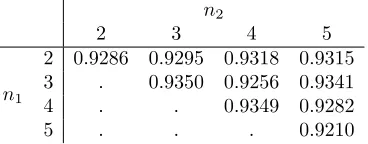
We observe thatmn1,n2(β) does not depend much ofn1, n2, as expected from Conjecture 3. This also guarantees that the value ofϑhas been conjectured correctly. Variations in the values ofmn1,n2(β) can be dismissed as random fluctuations and finite-size effects.
To summarise, we have studied numerically the joint distribution of the lengths of macro-scopic loops in a family of loop models in three dimensions. These loop models are motivated by their close relations to certain quantum spin systems and include in particular the ran-dom interchange model. We have observed the presence of the Poisson-Dirichlet distribution with parametersϑ= 1 and 1
[image:10.612.207.392.481.552.2]n2
2 3 4 5
n1
2 0.9576 0.9579 0.9562 0.9593 3 . 0.9671 0.9600 0.9580
4 . . 0.9539 0.9479
[image:11.612.220.405.119.189.2]5 . . . 0.9523
Table 3. Numerical values ofmn1,n2(β) foru= 0.5,β = 1, andL= 160. Here,mL(β) = 0.949.
n2
2 3 4 5
n1
2 0.9286 0.9295 0.9318 0.9315 3 . 0.9350 0.9256 0.9341
4 . . 0.9349 0.9282
5 . . . 0.9210
Table 4. Numerical values ofmn1,n2(β) for u= 1, β = 1, andL = 160. Here,mL(β) = 0.925.
Acknowledgments: We are grateful to Stefan Wessel for sending us the result of his numerical calculation of the critical temperature of the quantum XY model.
References
[1] M. Aizenman, B. Nachtergaele, Geometric aspects of quantum spin states, Comm. Math. Phys., 164, 17–63 (1994)
[2] G. Alon, G. Kozma,The probability of long cycles in interchange processes, to appear in Duke Math J.; arXiv:1009.3723 [math.PR]
[3] O. Angel, Random infinite permutations and the cyclic time random walk, Discrete Math. Theor. Comput. Sci. Proc., 9–16 (2003)
[4] N. Berestycki, Emergence of giant cycles and slowdown transition in random transpositions and k -cycles, Electr. J. Probab. 16, 152–173 (2011)
[5] N. Berestycki, G. Kozma, Cycle structure of the interchange process and representation theory, to appear in Bull. Soc. Math. France; arXiv:1205.4753 [math.PR]
[6] V. Betz, D. Ueltschi,Spatial random permutations and Poisson-Dirichlet law of cycle lengths, Electr. J. Probab. 16, 1173–1192 (2011)
[7] S. Friedli, Y. Velenik,Equilibrium Statistical Mechanics of Classical Lattice Systems: a Concrete In-troduction, in preparation, available at http://www.unige.ch/math/folks/velenik/smbook/
[image:11.612.222.406.241.313.2][8] C. Goldschmidt, D. Ueltschi, P. Windridge, Quantum Heisenberg models and their probabilistic rep-resentations, in Entropy and the Quantum II, Contemp. Math. 552, 177–224 (2011); arXiv:1104.0983 [math-ph]
[9] S. Grosskinsky, A.A. Lovisolo, D. Ueltschi,Lattice permutations and Poisson-Dirichlet distribution of cycle lengths, J. Statist. Phys. 146, 1105–1121 (2012)
[10] A. Hammond,Sharp phase transition in the random stirring model on trees, Probab. Theory Relat. Fields 161, 429–448 (2015)
[11] T.E. Harris,Nearest-neighbor Markov interaction processes on multidimensional lattices, Adv. Math. 9, 66–89 (1972)
[12] J.F.C. Kingman,Random discrete distributions, J. Royal Statist. Soc. B 37, 1–22 (1975)
[13] A. Nahum, J.T. Chalker, P. Serna, M. Ortu˜no, A.M. Somoza,Length distributions in loop soups, Phys. Rev. Lett. 111, 100601 (2013)
[15] O. Schramm,Compositions of random transpositions, Israel J. Math. 147, 221–243 (2005)
[16] B. T´oth,Improved lower bound on the thermodynamic pressure of the spin1/2Heisenberg ferromagnet, Lett. Math. Phys. 28, 75–84 (1993)
[17] M. Troyer, F. Alet, S. Wessel,Histogram methods for quantum systems: from reweighting to Wang-Landau sampling, Braz. J. Phys. 34, 377 (2004)
[18] D. Ueltschi,Random loop representations for quantum spin systems, J. Math. Phys. 54, 083301 (2013) [19] D. Ueltschi, Ferromagnetism, antiferromagnetism, and the curious nematic phase of S=1 quantum
spin systems, Phys. Rev. E 91, 042132 (2015)
[20] A. V¨oll, S. Wessel,Spin dynamics of the bilinear-biquadraticS= 1Heisenberg model on the triangular lattice: A quantum Monte Carlo study, Phys. Rev. B 91, 165128 (2015)
[21] S. Wessel, private communication
Department of Physics, University of Warwick, Coventry, CV4 7AL, United Kingdom E-mail address: [email protected]
Department of Physics, University of Warwick, Coventry, CV4 7AL, United Kingdom E-mail address: [email protected]
Department of Statistics, University of Oxford, 1 South Parks Road, Oxford OX1 3TG, United Kingdom
E-mail address: [email protected]