Model based clustering using copulas with applications

warwick.ac.uk/lib-publications

Kosmidis, Ioannis and Karlis, D.. (2016) Model-based clustering using copulas with applications. Statistics and Computing, 26 (5). pp. 1079-1099.

Permanent WRAP URL:

http://wrap.warwick.ac.uk/98830

Copyright and reuse:

The Warwick Research Archive Portal (WRAP) makes this work by researchers of the University of Warwick available open access under the following conditions. Copyright © and all moral rights to the version of the paper presented here belong to the individual author(s) and/or other copyright owners. To the extent reasonable and practicable the material made available in WRAP has been checked for eligibility before being made available.

Copies of full items can be used for personal research or study, educational, or not-for profit purposes without prior permission or charge. Provided that the authors, title and full bibliographic details are credited, a hyperlink and/or URL is given for the original metadata page and the content is not changed in any way.

Publisher’s statement:

The final publication is available at Springer via https://doi.org/10.1007/s11222-015-9590-5

A note on versions:

The version presented here may differ from the published version or, version of record, if you wish to cite this item you are advised to consult the publisher’s version. Please see the ‘permanent WRAP url’ above for details on accessing the published version and note that access may require a subscription.

Model-based clustering using copulas with applications

Ioannis Kosmidis

Department of Statistical Science, University College London

Gower Street, WC1E 6BT, London, UK

and

Dimitris Karlis

Department of Statistics, Athens University of Economics and Business

76 Patision Str, 10434, Athens, Greece

July 3, 2015

Abstract

The majority of model-based clustering techniques is based on multivariate Normal models and their variants. In this paper copulas are used for the construction of flex-ible families of models for clustering applications. The use of copulas in model-based clustering offers two direct advantages over current methods: i) the appropriate choice of copulas provides the ability to obtain a range of exotic shapes for the clusters, and ii) the explicit choice of marginal distributions for the clusters allows the modelling of multivariate data of various modes (either discrete or continuous) in a natural way. This paper introduces and studies the framework of copula-based finite mixture mod-els for clustering applications. Estimation in the general case can be performed using standard EM, and, depending on the mode of the data, more efficient procedures are provided that can fully exploit the copula structure. The closure properties of the mix-ture models under marginalization are discussed, and for continuous, real-valued data parametric rotations in the sample space are introduced, with a parallel discussion on parameter identifiability depending on the choice of copulas for the components. The exposition of the methodology is accompanied and motivated by the analysis of real and artificial data.

Keywords: mixture models; dependence modelling; parametric rotations; multivariate discrete data; mixed-domain data.

1

Introduction

1.1

Finite Mixture models for real-valued data

The use of finite mixture models in clustering is finding a large number of applications, mainly because it allows standard statistical modelling tools to be used in order to assess and evaluate the clustering. The density or probability mass function of a finite mixture model is defined as

h(x;θ,π) = k

X

πjfj(x;θj) (x∈ <p), (1)

where θ = (θ>₁, . . . ,θ_k>)> _{∈ Θ}

1 ×. . .×Θk, and πj ∈ (0,1) with Pk_j=1πj = 1. Appropriate

choices of fj(x;θj) can result in flexible models of small complexity. Banfield and Raftery

(1993) and the book of McLachlan and Peel (2000) provide a detailed treatment of the framework of finite mixture modelling for clustering.

For continuous data, a common choice for the component densitiesfj(x;θj) (j = 1, . . . , k)

is the density of the multivariate Normal distribution. This is mainly because of the conve-nience it offers in estimation (closed-form maximization steps in the EM algorithm) and in-terpretation (easy marginalization for visualising fitted components and the mixture density). The resultant clusters, though, are limited to be elliptical in shape, and as is demonstrated in Hennig (2010), one may need more than one multivariate Normal components, in order to fit a single non-elliptical cluster.

Such restrictions of multivariate Normal finite mixtures have resulted in an expanding literature where other special component distributions are considered. Prominent

exam-ples of alternative component densities include multivariate t distributions (see, Andrews

and McNicholas, 2011), multivariate skew-Normal and skew-t distribution (see, for example,

Fr¨uhwirth-Schnatter and Pyne, 2010; Lee and McLachlan, 2014), multivatiate skew

student-t-Normal distributions (Lin et al., 2014), multivariate Normal inverse Gaussian distributions

(Karlis and Santourian, 2009). Other attempts can be found in Forbes and Wraith (2014) for finite mixtures of multivariate scaled Normal distributions and (Morris and McNicholas, 2013) for mixtures of shifted asymmetric Laplace distributions. The results of such studies indicate that the introduction of heavy tails and/or skewness allows the construction of more parsimonious models than multivariate Normal mixtures, which can also bridge the gap be-tween the number of clusters present in the data and the number of components used in the mixture.

Despite the added flexibility that such mixture models offer, all of them force the data to obey very specific marginal properties, and they are not appropriate, for example, in cases where the simultaneous treatment of real-valued observations, strictly positive and

observations in (0,1) is needed. In such cases one needs to either ignore the range of the

variables and treat them as real-valued or apply appropriate transformations that map the original range of the observations on the real line. Furthermore, even for real-valued variables, as Example 1.1 illustrates, current methods can fail to capture certain dependence structures.

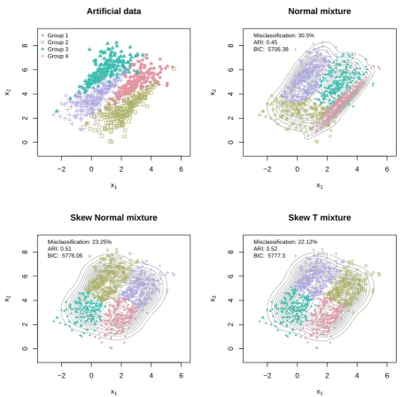
Example 1.1: Consider the artificial data set shown in the top left plot of Figure 1. The

data set is formed by four distinct clusters of observations each shown in a different colour on the plot. A Clayton and a survival Clayton copula with Normal marginals has been used for generating Groups 3 and 4, and then an exact copy of the latter has been translated appropriately in order to form Groups 1 and 2.

In an attempt to reconstruct the true groups, the data set was fitted using a bivariate Normal mixture model, a bivariate skew-Normal mixture model, and a bivariate skew-t mix-ture model. All fitting procedures were initialized by the best k-means clustering in four clusters after 1000 random starting points. The resulting classification plots are shown in Figure 1. Each plot also provides the value of the Bayesian Information Criterion (BIC) for each model and the corresponding misclassification rate. As is apparent none of the three models performs well in detecting the true shape of the underlying clusters with the

misclas-sification rates ranging between 22.12% to 30.5% and adjusted Rand index (ARI) between

0.45 and 0.51.

● ● ● ● ● ● ● ● ● ● ● ● ● ● ● ● ● ● ● ● ● ● ● ● ● ● ●● ● ● ● ● ● ● ● ● ● ● ● ● ● ● ● ● ● ● ● ● ● ● ● ● ● ● ● ● ● ● ● ● ● ● ● ● ● ● ● ● ● ● ● ● ● ● ● ● ● ● ● ● ● ● ● ● ● ● ● ● ● ● ● ● ● ● ● ● ● ● ● ●● ● ● ● ● ● ● ● ● ● ● ● ● ● ● ● ● ● ● ● ● ● ● ● ● ● ● ● ● ● ● ● ● ● ● ● ● ● ● ● ●● ● ● ● ● ● ● ● ● ● ● ● ● ● ● ● ● ● ● _● ● ● ● ● ● ● ● ● ● ● ● ● ● ● ● ● ● ● ● ● ● ● ● ● ● ● ● ● ● ● ● ● ● ● ● ● ● ● ●

−2 0 2 4 6

0 2 4 6 8 x1 x2 Artificial data

● Group 1 Group 2 Group 3 Group 4 x1 x2 0.0041 0.0082 0.0123 0.0164 0.0205 0.0246 0.0287 0.0328 0.0369 0.041 0.041 0.0451 0.0451

−2 0 2 4 6

0 2 4 6 8 Normal mixture ● ● ● ● ● ● ● ● ● ● ● ● ● ● ● ● ● ● ● ●● ● ● ● ● ● ●● ● ● ● ● ● ● ● ● ● ● ● ● ● ● ● ● ● ● ● ● ● ●● ● ● ● ● ● ● ● ● ● ● ● ● ● ● ● ● ● ● ● ● ● ● ● ● ● ● ● ● ● ● ● ● ● ● ● ● ●● ● ● ● ● ● ● ● ● ● ● ● ● ● ● ● ● ● ● ● ● ● ● ● ● ●● ● ● ● ● ● ● ● ● ● ● ● ● ● ● ● Misclassification: 30.5% ARI: 0.45

BIC: 5706.38

x1 x2 0.0036 0.0072 0.0107 0.0143 0.0179 0.0215 0.0251 0.0286

0.0322 0.0358 0.0394 0.0429 0.0465 0.0501 0.0501

−2 0 2 4 6

0

2

4

6

8

Skew Normal mixture

● ● ● ● ● ● ● ● ●● ● ● ● ● ● ● ● ● ● ● ● ● ● ● ● ● ● ● ● ● ● ● ● ● ● ● ● ● ● ● ● ● ● ● ● ● ● ● ● ● ● ● ● ● ● ● ● ● ● ● ● ● ● ● ● ● ● ● ● ● ● ●● ● ● ● ● ● ● ● ● ● ● ● ● ● ● ● ● ● ● ● ● ● ● ● ● ● ● ● ● ● ● ● ● ● ● ● ● ● ● ● ● ● ● ● ● ●● ● ● ● ● ● ● ● ● ● ● ● ● ● ● ● ● ● ● ● ● ● ● ● ● ● ● ● ● ● ● ● ● ● ● ● ● ● ● ● ● ● ● ● ● ● ● ● ● ● ● ● ●● ● ● ● ● ● Misclassification: 23.25% ARI: 0.51

BIC: 5776.06

x1 x2 0.0034 0.0068 0.0102 0.0136 0.0169 0.0203 0.0237 0.0271

0.0305 0.0339 0.0373 0.0407 0.044 0.0474 0.0474

−2 0 2 4 6

0

2

4

6

8

Skew T mixture

● ● ● ● ● ● ● ● ● ● ● ● ● ● ● ● ● ● ● ● ● ● ● ● ● ● ● ● ● ● ● ● ● ● ● ● ● ● ● ● ● ● ● ● ● ● ● ● ● ● ● ● ● ● ● ● ● ● ● ● ● ● ● ● ● ● ● ● ● ● ● ● ●● ● ● ● ● ● ● ● ● ● ● ● ● ● ● ● ● ● ● ● ● ● ● ● ● ● ● ● ● ● ● ● ● ● ● ● ● ● ● ● ● ● ● ● ● ● ● ● ●● ● ● ● ● ● ● ● ● ● ● ● ● ● ● ● ● ● ● ● ● ● ● ● ● ● ● ● ● ● ● ● ● ● ● ● ● ● ● ● ● ● ● ● ● ● ● ● ● ● ● ● ●● ● ● ● ● ● ● Misclassification: 22.12% ARI: 0.52

BIC: 5777.3

Figure 1: An artificial data set with observations on two continuous variables (top left), a fitted mixture of four 2-dimensional Normal distributions (top right), a fitted mixture of four 2-dimensional skew-Normal distributions (bottom left) and a fitted mixture of four 2-dimensional skew-t distributions (bottom right).

1.2

Finite mixture models for clustering non-continuous data

For non-continuous data, one needs to specify fj(x;θj) (j = 1, . . . , k) in (1) through

prob-ability mass functions. While there is a wealth of choices for univariate non-continuous dis-tributions, the use of multivariate non-continuous distributions for the definition of mixture models is limited due to the difficulty in constructing easy to work with models that allow practical flexibility on the dependence structure. Some successful, but limited in application examples, are finite mixtures of multivariate Poisson distributions (Karlis and Meligkotsidou, 2007), finite mixtures of multinomial distributions (Jorgensen, 2004) and models based on conditionally independent Poisson distributions (see, for example Alfo et al., 2011). Mixture models with latent structures have been considered in Browne and McNicholas (2012), but these can have limitations because of assumptions like conditional independence.

1.3

Setting and fitting flexible finite mixture models

Subsections 1.1 and 1.2 highlight the need for a new framework for setting and fitting mixture models, which can i) match the flexibility that current proposals offer, and ii) can accommo-date the modelling of data with either continuous or non-continuous domains.

Copulas offer the means for constructing such a framework; their extensive use in the modelling of applications with multivariate data is due to the flexibility they offer in de-scribing dependence and in that they allow the construction of multivariate models with prescribed marginals. Nelsen (2006) provides an introduction to the concept of copulas.

Moreover, specifically for continuous data, common dependence measures like Kendall’s τ

and Spearman’s ρ are marginal-free and depend solely on the copula. This fact allows the

easy construction of multivariate mixture models for continuous data by first selecting the marginal properties of the variables involved and then the dependence structure implied by the mixture components.

A few attempts have already been made in the direction of facilitating the flexibility that copulas offer in model-based clustering (see, for example Jajuga and Papla, 2006; Di Lascio and Giannerini, 2012; Vrac et al., 2012). The current paper sets a thorough framework for constructing mixture models using copulas, highlighting the benefits but also the challenges of their use in practice. The ingredients for constructing copula-based mixture models are described in Section 2. Section 3 provides the details for maximum likelihood estimation through Expectation-Maximization (EM) algorithm and proposes relevant procedures for

obtaining starting values from the combination of a partitioning algorithm (likek-medoids)

2

A flexible specification of mixture models

2.1

Mixture models through copulas

A copulaC(u1, . . . , up) is a distribution function with uniform marginals. The importance of

copulas in statistical modelling stems from Sklar’s theorem (see, Nelsen, 2006, §2.3), which

shows that every multivariate distribution can be represented via the choice of an appropriate copula and, more importantly, it provides a general mechanism to construct new multivariate models in a straightforward manner.

The copula-based mixture model is defined as in (1) but nowθj is partitioned as (γj>,ψ>j )>

and fj(x;θj) is the density (or probability mass function) corresponding to a distribution

function

Fj(x;ψj,γj) = Cj(G1(x1;γj1), . . . , Gp(xp;γjp);ψj) (j = 1, . . . , k), (2)

where G1, . . . , Gp are univariate marginal cumulative distribution functions. As far as the

model parameters are concerned,γj contains the parameter vectors γjt for all marginals for

jth component (t= 1, . . . , p) andψ_j contains the parameters of the copula used for the j-th

component.

2.2

Construction of mixture models for any type of marginals

The definition of the component densityFj through the choice of a copulaCj and the choice

of marginal distributionsG1, . . . , Gp leads to a flexible framework for model-based clustering

that according to Sklar’s theorem necessarily encompasses all known mixture models and allows the convenient construction of new mixture models that can handle any of continuous, discrete data.

Temporarily omitting the component index and suppressing the dependence on the

pa-rameters, assume that the density of the copula C(u1, . . . , up) exists and is c(u1, . . . , up) =

∂p_C(u

1, . . . , up)/∂u1. . . ∂up. Then the component density for continuous marginals is

f(x) = c(G1(x1), . . . , Gp(xp)) p

Y

t=1

gt(xt),

wheregt(x) =dGt(x)/dxis the density function for thetth marginal distribution. For discrete

data, the probability mass function is given in Panagiotelis et al. (2012, expression (1.2)), and results from finite differences of the distribution function as

P(x) =X d

sgn(d)C(G1(d1), . . . , Gp(dp)), (3)

withd= (d1, . . . , dp) vertices, where each dt is equal to eitherxt orxt−1 (t= 1, . . . , p), and

sgn(d) =

1, if dt=xt−1 for an even number of t’s

−1, if dt=xt−1 for an odd number oft’s .

3

Model fitting

3.1

Full Expectation Maximization algorithm

Suppose that a sample of n p-vectors x1, . . . ,xn is available, which are assumed to be

re-alizations of independent random variables X1, . . . ,Xn each with distribution with density

or probability mass function as defined by (1) and (2). The maximization of the likelihood

function based on that sample can be performed using the EM algorithm. At the`th iteration

of the algorithm:

• E-step: Calculate

w(_ij`+1)= π (`)

j fj(xi;θ(j`))

Pk

j=1π (`)

j fj(xi;θj(`))

(i= 1, . . . , n; j = 1, . . . , k).

• M-step 1: Set π_j(`+1) =Pn

i=1w (`+1)

ij /n (j = 1, . . . , k).

• M-step 2: Maximize

k

X

j=1 n

X

i=1

w_ij(`+1)log_{fj(xi;θj)} ,

with respect to θ to obtain an updated value θ(`+1) for the copula and marginal

pa-rameters.

The algorithm iterates between theE-stepand theM-stepuntil some convergence criterion

is satisfied. In all the examples in the current paper the termination criterion that is used

is that the relative increase _{l(θ(`+1)<sub>, π</sub>(`+1)_)−l(θ(`)<sub>, π</sub>(`)_)}/l(θ(`)<sub>, π</sub>(`)_{) of the log-likelihood}

l(θ, π) in two successive iterations is less than = 10−8_.

3.2

Computational details

3.2.1 Maximization step

For the general model defined by (1) and (2), M-step 2 of the EM iteration is generally

not available in closed-form and needs to be performed numerically. At the current level of generality, it is recommended to take advantage of the separable form of the complete-data

log-likelihood for mixture models, which allows to break down the maximization task into k

independent maximizations of weighted likelihoods

θ_j(`+1) = arg max

Θj n

X

i=1

w_ij(`+1)log{fj(xi;θj)} (j = 1, . . . , k),

that can be performed in parallel.

3.2.2 Starting values

For calculating the starting values forπandθthe following procedure is proposed which takes

method (Joe, 1997, Chapter 10) for each component, and relies on an initial classification

vector that partitions the observation indicesA=_{1, . . . , n_}into exclusive subsetsS1, . . . , Sk,

with∪k

j=1Sj =A, of cardinalityN1, . . . , Nk, respectively. More specifically, the procedure for

obtaining starting values consists of the following steps:

S1 Set the starting values forπj using πj∗ =Nj/n (j = 1, . . . , k).

S2 Use maximum likelihood to fit the marginalgton data xit for i∈Sj in order to obtain

starting values γ_jt∗ for γjt (t= 1, . . . , p).

S3 Use maximum likelihood to fit the copula Cj(u1, . . . , up;ψj) on observations uit =

Gt(xit;γjt∗) (i ∈ Sj; t = 1, . . . , p), in order to get starting values ψ∗j for the copula

parameters ψj.

The initial classification vector can be obtained either using a hard-partitioning

distance-based algorithm (like k-means for continuous data or k-medoids more generally) or by

ran-domly sampling k observations and using the minimum distance of each to all other

obser-vations in order to form S1, . . . , Sk.

3.2.3 Choice of component ordering

The possibility of using different copulas for the components of the mixture model defined by (1) and (2), and the fact that the likelihood function for mixture models generally has local maxima, make the solution of the EM algorithm to depend on the order that the copulas appear in the mixture.

A solution to this problem is to fit all models that result from all possible permutations of the component copulas. Then, for each one of the unique permutations of the components, the procedure in Subsection 3.2.2 is applied, taking care to use the same initial classification

vector (and labelling) for A across permutations. Then the fitted model with the largest

value for the maximized log-likelihood is chosen. Example 4.1 below, uses this procedure for the choice of component ordering. Subsection 4.3.2 presents an alternative, less intensive solution, which can give rise to flexible mixture models without the need of considering many different candidate copulas for the components. That solution is based on extending the specification of the mixture model by allowing for component-wise parametric rotations.

If the same copula is used across the components of the mixture model, then the sensitivity that the result of the EM algorithm can have on the starting values can be alleviated by

trying several of those. This can be done by choosing a number of sets of k randomly

sampled observations, and construct distinct classification vectors by minimum distance, as described in Subsection 3.2.2. Then, for each vector, component-wise IFM is used to get the corresponding set of starting values and initialize the EM iterations. The model fit with the largest maximized log-likelihood is the one that is kept. The above process is used to carry out the analyses in Example 4.2 and Example 6.1.

4

Continuous data

4.1

Maximization step

• M-step 2: Maximize the log-likelihood

k

X

j=1 n

X

i=1

w(_ij`+1)

"

logcj(G1(xi1;γj1), . . . , Gp(xip;γjp);ψj) + p

X

t=1

loggt(xit;γjt)

#

, (4)

with respect toψ1, . . . ,ψk,γ11, . . . ,γ1p,γk1, . . . ,γkp, where γjt is the vector of parameters of

thetth marginal distribution for thejth component of the mixture (t= 1, . . . , p;j = 1, . . . , k).

As is apparent from (4) the only necessary ingredients for implementing the EM algorithm for mixtures of copulas for continuous data are the specification of the copula densities

c1, . . . , ck and the specification of the marginal density and distribution functions g1, . . . , gp and G1, . . . , Gp , respectively.

The particular form of the complete data log-likelihood for continuous data allows here the use of the Expectation/Conditional Maximization (ECM) algorithm of Meng and Rubin (1993), where the full maximization of the complete data log-likelihood is relaxed to max-imization in blocks; first with respect to the marginal parameters given the current value of the copula parameter and then with respect to the copula parameter given the updated

values for the marginal parameters. In mathematical notation,M-step 2 in Subsection 3.1 is

replaced by the steps

• CM-step 1: Maximize

k

X

j=1 n

X

i=1

w(_ij`+1)

"

logcj(G1(xi1;γj1), . . . , Gp(xip;γjp);ψj(`)) + p

X

t=1

loggt(xit;γjt)

#

, (5)

with respect to γ₁₁, . . ., γ_1p, γ_k1, . . ., γ_kp to obtain updated values γ₁₁(`+1), . . ., γ<sub>1</sub>(`_p+1),

γ_k(`<sub>1</sub>+1), . . .,γ<sub>kp</sub>(`+1) for the marginal parameters.

• CM-step 2: Maximize

k

X

j=1 n

X

i=1

w_ij(`+1)hlogcj(G1(xi1;γj(1`+1)), . . . , Gp(xip;γjp(`+1));ψj)

i

, (6)

with respect to ψ1, . . . ,ψk to obtain updated values ψ1(`+1), . . . ,ψ

(`+1)

k for the copula

parameters.

According to the definitions and results in Meng and Rubin (1993), the ECM algorithm

that results by replacing M-step 2 with the pair CM-step 1 and CM-step 2 shares all the

convergence properties of the full EM algorithm, and, in this particular case, is more

com-putationally efficient and stable, because CM-step 2 consists of a simple maximization with

respect to the copula parameters. Furthermore,CM-step 1 and CM-step 2 can each be

bro-ken down into parallel optimizations across components, as in the case of the full EM in Subsection 3.2, which significantly reduces computation time in multicore systems.

The pair of CM-step 1 and CM-step 2 is similar to the IFM method for fitting the

com-plete data likelihood. Their difference lies in CM-step 1 where instead of maximizing the

Example 4.1: Consider the setting of Example 1.1. The Normal mixture model failed to capture the dependence structure that is apparent in the true groups because of the strict elliptical shape of the component densities. Furthermore, two of the fashionable methods that allow non-elliptical clusters (mixtures of skew-Normals and skew-t distributions) were not able to recover the dependence structure of the groups in the artificial data.

The Gumbel copula and the Clayton copula can capture varying degrees of upper and lower tail dependence respectively and for the purposes of this example we consider a mixture model of two Gumbel copulas and two Clayton copulas with Normal marginals. The Gumbel copula is defined as

C(G)(u1, u2;ψ) = exp

h

−

(₋logu1)ψ + (−logu2)ψ

1/ψi

, ψ _∈[1,_∞), (7)

and the Clayton copula is defined as

C(C)_(u

1, u2;ψ) =

u−₁ψ+u−₂ψ₋1−1/ψ , ψ _∈(0,_∞). (8)

The associated densities c(G)_(u

1, u2;ψ) and c(C)(u1, u2;ψ) can be obtained by direct

differ-entiation of C(G)_(u

1, u2;ψ) and C(C)(u1, u2;ψ), respectively. The closed form expressions of

those copula densities are given in Hofert et al. (2012, Corollary 1) along with the correspond-ing expressions for other Archimedean copulas of arbitrary dimension. Then the density of the bivariate mixture model with two Gumbel and two Clayton components and Normal marginal distributions can be written as

h(x;θ,π) = 2

X

j=1

πjc(G)

Φ

x1−µj1

σj1

,Φ

x2−µj2

σj2

;ψj

2 Y

t=1 1

σjt

φ

xt−µjt

σjt

(9)

+ 4

X

j=3

πjc(C)

Φ

x1−µj1

σj1

,Φ

x2−µj2

σj2

;ψj

2 Y

t=1 1

σjt

φ

xt−µjt

σjt

,

where θ= (µ11, σ11, µ12, σ12, ψ1, . . . , µ41, σ41, µ42, σ42, ψ4)> and π= (π1, . . . , π4)> with

P4

j=1πj = 1. The functions Φ(.),φ(.) are the distribution and density function of a standard

Normal random variable, respectively.

Then M-step 2 of the maximization step at the `th iteration of the EM algorithm in

Subsection 3.1 consists of the maximization of each one of

n

X

i=1

w(_ir`+1)

"

logc

Φ

xi1−µr1

σr1

,Φ

xi2−µr2

σr2

;ψr

− 2

X

t=1

logσrt+

1 2

2

X

t=1

xit−µrt

σrt

2#

(10)

forr _{∈ {}1,2,3,4_}, wherec_≡c(G) _{for r∈ {1,2} and c≡c}(C) _{for r∈ {3,4}. For deriving the}

ECM algorithm in Subsection 4.1, each of those maximizations should be replaced by the

maximization of the function given in (10), firstly on with respect to µr1, σr1, µr2, σr2 at the

current valueψ(r`) of the copula parameter, in order to obtain updated marginal parameters

µ(_r`<sub>1</sub>+1), σ<sub>r</sub>(`₁+1), µ(_r`<sub>2</sub>+1), σ<sub>r</sub>(`₂+1), and, then, the maximization of

n

X

i=1

w(_ir`+1)logc

(

Φ xi1−µ

(`+1) r1

σ_r(`₁+1)

!

,Φ xi2 −µ (`+1) r2

σ(_r`₂+1)

!

;ψr

)

Component 1 Component 2 Component 3 Component 4

Gumbel Gumbel Clayton Clayton

Mixing probabilities πˆ1 = 0.24 πˆ2 = 0.24 πˆ3 = 0.25 πˆ4 = 0.27

Marginal parameters ˆ

µ11 = 2.31 µˆ21= 0.35 µˆ31= 2.79 µˆ41 = 0.78 ˆ

σ11= 0.95 σˆ21 = 0.97 σˆ31= 1.00 σˆ41= 1.02 ˆ

µ12 = 2.73 µˆ22= 3.76 µˆ32= 4.77 µˆ42 = 5.77 ˆ

σ12= 1.03 σˆ22 = 1.05 σˆ32= 1.05 σˆ42= 1.07

Copula parameters ψˆ1 = 2.86 ψˆ2 = 2.85 ψˆ3 = 3.56 ψˆ4 = 3.24

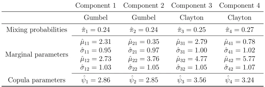
Table 1: Maximum likelihood estimates for the parameters for the mixture (9).

with respect toψr to obtain an updated value ψr(`+1) for the copula parameter. The latter is

simply a maximization with respect to the scalar parameter ψr and can be performed using

line search in the domain of definition of the copula parameter.

In the current example, the possible permutations of the copulas for the components are _{G, G, C, C_}, _{G, C, G, C_}, _{G, C, C, G_}, _{C, G, G, C_}, _{C, G, C, G_}, and _{C, C, G, G_},

where G and C stand for Gumbel and Clayton, respectively. Table 1 shows the estimates

for the parameters for that permutation of copulas which resulted in the largest maximized log-likelihood.

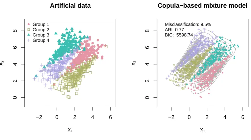
The resulting classification plot is shown in Figure 2. As is apparent the copula-based mixture model is performing very well in capturing the shape of the original clusters; the

misclassification rate is 9.5% and the BIC value (5598.74) has greatly improved from the

models in Figure 1. The resultant clustering has ARI of 0.77 which dominates the clusterings obtained in 1.1.

4.2

Bounded- and mixed-domain variables

The decoupling of the dependence properties from the marginal ones allows the easy construc-tion of multivariate mixture models for bounded-domain data (like percentages or strictly positive variables).

Mixture models for such data are usually formed from component densities defined by the product of independent univariate densities of appropriate support. Those models imply that the univariate marginal distributions of the component densities are independent conditional on the component membership. In effect, such models attempt to capture the dependence in the data only through the mixing probabilities. For example, Dean and Nugent (2013) define multivariate Beta mixture models in this way, and use them highlighting that the implied conditional independence assumption can be rather restrictive in practice.

Under the current framework, models with more complex dependence can be defined by

simply setting the component copula densities cj in (4), and choosing marginals with the

required support.

● ● ● ● ● ● ● ● ● ● ● ● ● ● ● ● ● ● ● ● ● ● ● ● ● ● ●● ● ● ● ● ● ● ● ● ● ● ● ● ● ● ● ● ● ● ● ● ● ● ● ● ● ● ● ● ● ● ● ● ● ● ● ● ● ● ●● ● ● ● ● ● ● ● ● ● ● ● ● ●● ● ● ● ● ● ● ● ● ● ● ● ● ● ● ● ● ● ●● ● ● ● ● ● ● ● ● ● ● ● ● ● ● ● ● ● ● ● ● ● ● ● ● ● ● ● ● ● ●● ● ● ● ● ● ● ● ● ●● ● ● ● ● ● ● ● ● ● ● ● ● ● ● ● ● ● ● _● ● ● ● ● ● ● ● ● ● ● ● ● ● ● ● ● ● ● ● ● ● ● ● ● ● ● ● ●● ● ● ● ● ● ● ● ● ● ●

−2 0 2 4 6

0 2 4 6 8 x1 x2 Artificial data

● _{Group 1} Group 2 Group 3 Group 4 x1 x2 0.0049 0.0099 0.0148 0.0198 0.0198 0.0247 0.0247 0.0296 0.0296 0.0296 0.0346 0.0346 0.0346 0.0395 0.0395 0.0445

−2 0 2 4 6

0

2

4

6

8

Copula−based mixture model

● ● ● ● ● ● ●● ● ● ● ● ● ● ● ● ● ● ● ● ● ● ● ● ● ● ● ● ● ● ● ● ● ● ● ● ● ● ● ● ● ● ● ● ● ● ● ● ● ● ● ● ● ● ● ● ● ● ● ● ●● ● ● ● ● ● ● ● ● ● ● ● ● ● ● ● ● ● ● ● ● ● ● ● ● ● ● ● ● ● ● ● ● ● ● ● ● ● ● ● ● ● ● ● ● ● ● ● ● ● ● ● ● ● ● ●● ● ● ● ● ● ● ● ● ● ● ● ● ● ● ● ● ● ● ● ● ● ● ● ● ● ● ● ● ● ● ● ● ● ● ● ● ● ● ● ● ● ● ● _● ● ● ● ● ● ● ● ● ● ● ● ● ● ● ●● ● ●● ● ● ● ● ● ● Misclassification: 9.5% ARI: 0.77

BIC: 5598.74

Figure 2: The artificial data set of Example 1.1 (left) and the contours of the fitted mixture of the bivariate mixture model with two Gumbel and two Clayton components and Normal marginal distributions (right).

Example 4.2: Hoopdata.com is a website that was launched in 2009 and provides an

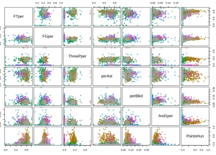
exten-sive database for NBA statistics. We used Hoopdata.com’s database to gather data for the scoring behaviour of the 493 NBA players that had more than 24 minutes game time (which accounts for half a game played in full) in the 2011-2012 season. For each player, the data has observations for the season free throws percentage (“FTper”), the field goals percentage (“FGper”), the three point percentage (“ThreePper”), the percentage of field goals assisted, the percentage blocked, the percentage of “And1” field goals, and the total points scored in hundreds (“PointsHun”). The aim of the analysis is to form groups of players in terms of their performance.

For all players that had observation 0% or 100% in any of the percentages, the observation

is replaced by 0.01% and 99.99%, respectively. After making the substitutions, the free

throws, the field goals and the three point percentages take values in (0,1). Furthermore, the

points scored are all positive. Plausible marginal specifications are a Beta distribution for modelling each of the percentage variables and a Gamma distribution for modelling the points scored. Then we use a 7-variate Gaussian copula for modelling the dependence between the 7 variables.

The multivariate Gaussian copula with correlation matrixR is defined as

C(N)(u1, . . . , up;R) = Φp(Ψ(u1), . . . ,Ψ(up);R), (11)

where Φp(., . . . , .) is the distribution function of a standard p-variate Normal distribution

Normal distribution. The matrixR has the general form

R =

    

1 ρ12 . . . ρ1p

ρ12 1 . . . ρ2p

... ... ... ...

ρ1p ρ2p . . . 1

    

, (12)

whereρtt0 ∈[−1,1] is the correlation between thetth and t0th variable (t, t0 ∈ {1, . . . , p};t 6=

t0_).

For the current case the density of the mixture model to be fitted is

k

X

j=1

πjφ7[Ψ{Gj1(x1)}, . . . ,Ψ{Gj7(x7)};Rj] 7

Y

t=1

gjt(xt)

φ1[Ψ{Gjt(xt)}]

, (13)

where φp is the density of a p-dimensional standard Normal distribution and gjt(x) =

∂Gjt(x)/∂x, where for t ∈ {1, . . . ,6}, Gjt(x) is the distribution function of a Beta

ran-dom variable with shape parametersαjt, and Gj7(x) is the distribution function of a Gamma

random variable with shape parameter κj and scale 1/λj. More specifically, the density

functions for the marginals are

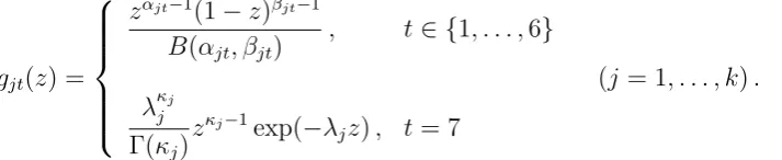
gjt(z) =

          

zαjt−1_(1−z)βjt−1

B(αjt, βjt)

, t_{∈ {}1, . . . ,6_}

λκj_j

Γ(κj)

zκj−1exp(−λjz), t= 7

(j = 1, . . . , k).

The matrix Rj has exactly the same structure as the matrix R in (12) but the correlations

depend onj ensuring that each component in the mixture can accommodate different

corre-lation structures. Hence, the parameters to be estimated are αj1, βj1, . . ., αj6, βj6, κj and

λj for the marginals of the jth component, ρ12,j, . . .,ρ17,j, . . ., ρ67,j for the copula of the jth

component (j = 1, . . . , k) and the mixing proportions π1, . . . , πk−1. Hence, the model in (13)

has q = 36k₋1 free parameters. The number of free parameters can be further reduced by

fitting models nested to (13) that have a structured correlation matrix. For example, a nested

model to (13) with 16k−1 parameters can be formed by considering exchangeable correlation

for each component where all correlations appearing inRj are equal to ρj (j = 1, . . . , k).

Fork= 2, . . . ,9, density (13) is fitted to the data on the NBA players with both unstruc-tured and exchangeable correlation. For the models with exchangeable correlation and for

each k, 15 sets of starting values were obtained by selecting 15 sets of k randomly selected

observations for the intialization of the component-wise IFM procedure in Subsection 3.2.2. Then the model with the highest log-likelihood was chosen and was also used to initialise the model with unstructured correlation.

Furthermore, we restricted the variance of each of the Beta marginals involved in the

mixture to be greater than 10−4_{. In this way, unbounded likelihood values relating to}

obser-vations with the same percentage value can be avoided.

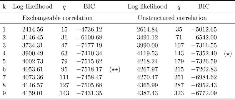
Table 2 lists the maximized log-likelihood, the number of parametersq and the BIC value

for the best 18 fitted mixtures. The model with exchangeable correlation matrix andk = 6

has the lowest BIC value.

The maximum of the weights wi1, . . . , wik at the last iteration of the EM algorithm (see

k Log-likelihood q BIC Log-likelihood q BIC

Exchangeable correlation Unstructured correlation

1 2414.56 15 −4736.12 2614.84 35 −5012.65 2 3146.45 31 ₋6100.68 3491.12 71 ₋6542.00 3 3734.31 47 ₋7177.19 3990.00 107 ₋7316.55 4 3900.49 63 −7410.34 4119.53 143 −7352.40 (?) 5 4002.73 79 ₋7515.62 4218.24 179 ₋7326.59 6 4053.61 95 ₋7518.17 (??) 4267.97 215 ₋7202.83 7 4073.36 111 −7458.47 4270.47 251 −6984.62 8 4146.57 127 ₋7505.68 4365.99 287 ₋6952.43 9 4159.01 143 ₋7431.35 4387.43 323 ₋6772.09

Table 2: Maximum likelihood fits of the density (13) for the data on the NBA players with

k∈ {2, . . . ,9} components for both unstructured and exchangeable correlation structure. A

(?) denotes the best BIC for each copula specification and a (??) the best BIC overall.

model with exchangeable correlation matrices and k = 6, Figure 3 shows the marginal

his-tograms of the observations within each cluster along with the marginal densities gjt(.) at

the maximum likelihood estimates for each cluster-variable combination. The agreement of the fitted marginals with the histograms of the variables indicates a good fit. Furthermore, Figure 3 shows that the fit has achieved some separation between the clusters, especially for “PointsHun”.

A “true classification” of the players in terms of performance is not generally available, so it is hard to check how good the resultant classification is. However, there is a wealth of metrics that attempt to capture different characteristics of the player. A few representa-tive metrics include the NBA Efficiency rating (“EFF”), the Usage Rate (“USG”), the True Shooting percentage (“TSper”), John Hollinger’s Player Efficiency Rating (“PER”) and

Al-ternative Win Score (“AWS”). Hoopdata.com provides the values for these metrics for each

player in the 2011-2012 season and we use these values to assess the comparative performance

of the copula-based mixture model to that of a Normal mixture fitted using themclust

(Fra-ley et al., 2012) R package as follows: each metric is broken intoI intervals, whose endpoints

are calculated using the empirical quantiles atI+ 1 equidistant probabilities ranging from 0

to 1. For each metric and for I _{∈ {}2, . . . ,30_}, we calculate the ARI of the clustering with 6

Beta and 1 Gamma marginal, and the ARI of the clustering from the Normal mixture model

with the lowest BIC (4 components with VEV parameterization with BIC −5026.44; VEV

stands for “variable volume, equal shape, variable orientation” and characterizes a particular parameterization for the variance-covariance matrix of the multivariate Normal distribution for the component distributions; see, Fraley et al. 2012 for the VEV and the other

param-eterizations that mclust uses). Figure 4 shows the results for each metric. Despite the low

ARI’s for both fits, all points fall below the 45o _{line and, hence, the clustering from the}

copula-based mixture model clearly dominates the one from the optimal Normal mixture model with regards to those metrics.

As a reviewer correctly pointed out, another way to handle clustering of bounded- or mixed-domain data is to first appropriately transform the data and then use standard mix-ture models for continuous data, such as Normal mixmix-tures. Dean and Nugent (2013)

Cluster 1

π

^

1=0.1

FTper

Density

0

5

10

15 _{Mean: 0.72}

SD : 0.07

FGper Density 0 5 10 15 20

25 _{Mean: 0.49}

SD : 0.04

ThreePper Density 0 5 15 25

35 _{Mean: 0.25}

SD : 0.34

perAst Density 0 5 15 25

35 _{Mean: 0.63}

SD : 0.13

perBlkd Density 0 5 15 25

35 _{Mean: 0.08}

SD : 0.03

And1per Density 0 5 15 25

35 _{Mean: 0.04}

SD : 0.02

PointsHun Density 0.0 0.4 0.8 Mean: 6.25 SD : 4.27

Cluster 2

π^

2=0.36

Density

0

5

10

15 _{Mean: 0.79}

SD : 0.07

Density 0 5 10 15 20

25 _{Mean: 0.43}

SD : 0.04

Density

0

5

15

25

35 _{Mean: 0.34}

SD : 0.06

Density

0

5

15

25

35 _{Mean: 0.55}

SD : 0.16

Density

0

5

15

25

35 _{Mean: 0.06}

SD : 0.02

Density

0

5

15

25

35 _{Mean: 0.02}

SD : 0.01

Density

0.0

0.4

0.8

Mean: 6.61 SD : 3.14

Cluster 3

π^

3=0.21

Density

0

5

10

15 _{Mean: 0.71}

SD : 0.13

Density 0 5 10 15 20

25 _{Mean: 0.39}

SD : 0.05

Density

0

5

15

25

35 _{Mean: 0.3}

SD : 0.09

Density

0

5

15

25

35 _{Mean: 0.64}

SD : 0.19

Density

0

5

15

25

35 _{Mean: 0.05}

SD : 0.03

Density

0

5

15

25

35 _{Mean: 0.01}

SD : 0.02

Density

0.0

0.4

0.8

Mean: 1.85 SD : 1.08

Cluster 4

π^

4=0.09

Density 0 5 10 15 Mean: 0.5 SD : 0.43

Density 0 5 10 15 20 25 Mean: 0.44 SD : 0.23

Density 0 5 15 25 35 Mean: 0.15 SD : 0.22

Density 0 5 15 25 35 Mean: 0.65 SD : 0.36

Density 0 5 15 25 35 Mean: 0.03 SD : 0.06

Density 0 5 15 25 35 Mean: 0.03 SD : 0.05

Density

0.0

0.4

0.8

Mean: 0.31 SD : 0.28

Cluster 5

π^

5=0.11

Density 0 5 10 15 Mean: 0.61 SD : 0.17

Density 0 5 10 15 20 25 Mean: 0.42 SD : 0.09

Density 0 5 15 25 35 Mean: 0.09 SD : 0.17

Density 0 5 15 25 35 Mean: 0.6 SD : 0.18

Density 0 5 15 25 35 Mean: 0.1 SD : 0.05

Density 0 5 15 25 35 Mean: 0.02 SD : 0.05

Density

0.0

0.4

0.8

Mean: 0.46 SD : 0.27

Cluster 6

π^

6=0.13

Density

0

5

10

15

0.0 0.4 0.8 Mean: 0.63 SD : 0.1

Density 0 5 10 15 20 25

0.0 0.4 0.8 Mean: 0.5 SD : 0.06

Density 0 5 15 25 35

0.0 0.4 0.8 Mean: 0 SD : 0.01

Density 0 5 15 25 35

0.0 0.4 0.8 Mean: 0.67 SD : 0.07

Density 0 5 15 25 35

0.0 0.4 0.8 Mean: 0.1 SD : 0.03

Density 0 5 15 25 35

0.0 0.4 0.8 Mean: 0.04 SD : 0.02

Density

0.0

0.4

0.8

0 5 15 25

Mean: 2.94 SD : 1.64

Figure 3: Mixture of 6 7-dimensional Gaussian copulas with exchangeable correlation matri-ces and 6 Beta and 1 Gamma marginals each. The plots show the marginal histograms of the observations within each cluster along with the fitted marginal densities for each

cluster-variable combination. The fitted mixing proportions ˆπi (i= 1, . . . ,6) are also reported.

● ● ● ●● ● ● ● ● ● ● ● ● ● ● ● ● ● ● ● ● ● ● ● ● ● ● ● ● ●

0.00 0.10 0.20

0.00 0.10 0.20 EFF Copula ARIs Mclust ARIs ● ● ● ●● ● ● ● ● ● ● ● ● ●● ● ● ● ● ● ● ● ● ● ● ● ● ●● ●

0.00 0.06 0.12

0.00 0.04 0.08 0.12 USG Copula ARIs Mclust ARIs ● ● ● _{● ●} ● ● ● ●● ● ● ● ● ● ● ● ● ● ● ● ● ● ●● ● ●●●●

0.00 0.04 0.08 0.12

0.00 0.04 0.08 0.12 TSper Copula ARIs Mclust ARIs ● ● ● ● ● ● ● ● ● ● ● ● ● ● ● ● ● ● ● ● ●● ● ● ● ● ● ● ● ●

0.00 0.05 0.10 0.15

0.00 0.05 0.10 0.15 PER Copula ARIs Mclust ARIs ● ● ● ● ● ● ● ● ● ● ● ● ● ● ● ● ● ● ● ● ● ● ● ● ● ● ● ● ● ●

0.00 0.10 0.20

0.00 0.10 0.20 AWS Copula ARIs Mclust ARIs

Figure 4: Clustering quality of best copula-based mixture model versus the best Normal

Normal mixture models on the transformed data. Their results indicate that treating the bounded-domain data with distributions that are defined on that domain produces better results (see, for example Dean and Nugent, 2013, Table 1, for the results of the simulation study). Another important reason for working with the bounded-domain data directly is for avoiding the arbitrariness of choice of transformation before fitting a mixture model. Sec-tion 1 of the supplementary material extends Example 4.2 to illustrate that distinct sensible, transformations can lead to different results.

4.3

Real-valued variables

4.3.1 Invariance with respect to affine transformations

Suppose that the n vectors x1, . . . ,xn of observations have real-valued components. Then,

the fit of a copula-based mixture model with marginal distributions in the location-scale family (like Normal, skew-Normal, Cauchy, t, logistic and so on) is invariant with respect to

the translation and component-wise scaling of x1, . . . ,xn. This is because the location and

scale of the components are determined only by the marginal distributions.

More formally, suppose that all marginals support the real line and that the fitted marginal

means and variances of the jth component based on data x1, . . . ,xn are ˆµj1, . . . ,µˆjp and

ˆ

σ2

j1, . . . ,σˆ2jp (j = 1, . . . , k), respectively. Then, if zi = a+Bxi (i = 1, . . . , n), where B is a diagonal matrix with non-zero diagonal entries, the fitted marginal means and variances

of the jth component based on data z1, . . . ,zn will simply be a +B11µˆj1, . . . , a+Bppµˆjp

and B2

11σˆ2j1, . . . , Bpp2 σˆ2jp (j = 1, . . . , k), respectively. This follows directly from the invariance properties of the maximum likelihood estimator.

However, depending on the choice of copulas, the same mixture will generally produce a

different clustering for general affine transformations of the formzi _=a+Bxi _{(i= 1, . . . , n),}

whereB is a general real-valued p_×p matrix. This is because a copula-defined distribution

is not necessarily closed under general affine transformations (for example rotations). In contrast closure under general affine transformations is satisfied for all mixture models that

are based on elliptical distributions such as Normal andt mixtures (Fang et al., 2002).

4.3.2 Rotated copulas

In two dimensions, the survival version of any copulaC(u1, u2) isC180(u1, u2) = u1+u2−1 +

C(u1, u2), where “180” denotes that the survival copula is a rotated version of C(u1, u2) by

180o clockwise. Similarly, counter-clockwise rotated versions ofC(u1, u2) by 90o and 270o can

be defined as functions ofC(u1, u2) and u1, u2. Expression for those are given in Brechmann

and Schepsmeier (2013). Hence, one can select an initial dictionary of copulas to be used and then to further enrich this dictionary with the rotated versions of the copulas.

Example 4.3: In Example 4.1 we chose the copulas for the components by recognising

the need for mixture components that can accommodate extreme tail dependence through inspection of the scatterplot of the data. In this respect, we chose to have two mixture components based on the Gumbel copula which exhibits upper tail dependence and two components based on the Clayton copula which exhibits lower tail-dependence. Since a

rotated version of the Clayton copula by 180o _{(survival Clayton) would exhibit upper tail}

error of 9.875% and a BIC value of 5561.73. Similarly, fitting a model with two Gumbel and

two survival Gumbel components gives misclassification error of 11.25% and a BIC value of

5644.36.

As is illustrated in Example 4.3, the ability to construct new copula families from known ones certainly adds great flexibility when constructing copula-based mixture models for clus-tering. However, it certainly does not simplify model selection in a mixture model framework;

if we limit ourselves to a dictionary of d copulas, then for finding the best model amongst

the models withk components we need to fit and select the best model from d+k_k−1

models. Furthermore, if the number of components is also considered as part of the model selection

exercise, then one needs to fit and comparePK

k=1

d+k−1 k

whereK is a preset maximum

num-ber of components. Both these numnum-bers increase quickly as either K or d increase possibly

making the model selection exercise impractical.

4.3.3 Component-wise parametric rotations

Subsections 4.3.1 and 4.3.2 show that the added flexibility from the use of mixture of copulas may come with the price of two shortcomings from a practitioners point of view: the general lack of invariance with respect to general affine transformations of the data, and the fact that completely different copulas can result in fits of comparable quality. The latter issue is not so serious provided that the computational resources are enough for fitting many models and keeping in mind the target of the analysis is to find a good model. Though it certainly points towards the direction that if one had a more flexible specification for the mixture components,

the number PK

k=1

d+k−1 k

of models that need to be fitted is significantly decreased because

d can be drastically reduced. The invariance issue is harder to tackle. However, a flexible

enough model could alleviate some of the invariance issues by maintaining the translation and scaling invariance of the component densities, and by allowing the component densities to rotate based on the observations.

Consider the mixture of copulas specified by (1) and (2) withp= 2. Temporarily omitting

the component index, each component density has the form

f(x∗;γ,ψ) =c(G1(x∗1;γ1), G2(x∗2;γ2);ψ)g1(x∗1;γ1)g2(x∗2;γ2), x∗ ∈ <2.

Now consider the transformation X =O(ω)X∗, where O(ω) is the rotation matrix

O(ω) =

cosω ₋sinω

sinω cosω

,

withω _∈(0,2π]. ThenX is a counter-clockwise rotation ofX∗ at an angleωand the density

function ofX is simply

f∗(x;γ,ψ, ω) = f(O(ω)>x;γ,ψ), x_{∈ <}2, (14)

because for any rotation matrixO(ω)−1 _=O(ω)> _{(O(ω) is orthonormal) and |detO(ω)|= 1.}

Hence, the contours off∗ will be a counter-clockwise rotation of the contours off at an angle

ω. Hence, in the two-dimensional case, an extended mixture model can be defined that has

the form

h(x;θ,ω) = k

X

j=1

The difference of the latter specification from the mixture model in (1) and (2) is that

there are an extra k rotation angles to be estimated, but the added flexibility is enormous.

The practitioner can now select the marginals and a much smaller dictionary of copulas;

notice that all versions of the rotated copulas by 90o_{, 180}o _{and 270}o _{are special cases for the}

components of model (15) for specific values of ω1, . . . , ωk and that other exotic bivariate

distributions may result for arbitrary angles.

The mixture model (15) can be fitted using the EM algorithm; the only modification from

the general iteration in Subsection 3.1 is that atM-step 2 of the `th iteration, the function

k

X

j=1 n

X

i=1

w_ij(`+1)

"

logcj(G1(zi1(ωj);γj1), . . . , Gp(zip(ωj);γjp);ψj) + p

X

t=1

loggt(zit(ωj);γjt)

#

,

(16)

is maximized with respect to γ11, . . . ,γ1p, . . . ,γk1, . . . ,γkp,ψ1, . . . ,ψk, ω1, . . . , ωk. In (16),

zi(ωj) = O(ωj)>xi where zi(ωj) = (zi1(ωj), . . . , zip(ωj))> (i = 1, . . . , n;j = 1, . . . , k). This

M-stepcan also be broken down into k independent optimizations.

In order to avoid maximization over a large parameter space, the ECM algorithm in

Subsection 4.1 can be extended for handling parametric rotations i) by replacing xit with

zit(ωj(`)) (t = 1, . . . , p) in CM-step 1 and CM-step 2, and ii) by including an additional last

step to update the angles at the values of the marginal and copula parameters fromCM-step

1and CM-step 2. In that last step the objective

k

X

j=1 n

X

i=1

w_ij(`+1)

"

logcj(G1(zi1(ωj);γj(`1+1)), . . . , Gp(zip(ωj);γjp(`+1));ψ (`+1)

j ) (17)

+ p

X

t=1

loggt(zit(ωj);γjt(`+1))

#

,

is maximized with respect to ω1, . . . , ωk to obtain updated values ω1(`+1), . . . , ω

(`+1)

k . As is

the case for CM-step 1 and CM-step 2, this last step can also be broken down into parallel

optimizations across components, each of which consists of a one-dimensional maximization with respect to the respective angle.

Example 4.4: As is illustrated in Example 4.3 one can fit a mixture of two Clayton and

two survival Clayton, or a mixture of two Gumbel and two survival Gumbel, or a mixture of two Gumbel and two Clayton copulas to the artificial data of Example 1.1 and obtain comparable fits in all cases. Hence, we have considered the combinations of four different copulas for the components so far. The whole modelling exercise is much easier if we pick just one copula which exhibits tail-dependence (upper or lower), and Normal marginals and use those for setting up the mixture density (15).

For example, using the Clayton copula one obtains the estimated angles ˆω1 = 180.41,

ˆ

ω2 = 180.78, ˆω3 = 7.13, ˆω4 = 359.99 and a misclassification error of 9.875%. Figure 5

shows the contours of the fitted component densities across the iterations of the ECM algo-rithm and demonstrates the enormous flexibility that parametric rotations offer when setting copula-based mixture models. Iteration 0 (top left) refers to the starting values for the ECM

algorithm. The BIC value for the fit that allows parametric rotations is 5585.372 which is

larger the 5561.73 of the mixture with two Clayton and two survival Clayton in Example 4.3.

● ● ● ● ● ● ● ● ● ● ● ● ● ● ● ● ● ● ● ● ● ● ● ● ● ● ● ● ● ● ● ● ● ● ● ● ● ● ● ● ● ● ● ● ● ● ● ● ● ● ● ● ● ● ● ● ● ● ● ● ● ● ● ● ● ● ● ● ● ● ● ● ● ● ● ● ● ● ● ● ● ● ● ● ● ● ● ● ● ● ● ● ● ● ● ● ● ● ● ● ● ● ● ● ● ● ● ● ● ● ● ● ●

−2 0 2 4

0 2 4 6 8 Iteration 0 x1 x2 0.005 0.01 0.015 0.02 0.025 0.03 0.04 0.005 0.01 0.015 0.02 0.025 0.03 0.035 0.04 0.005 0.01 0.015 0.02 0.025 0.03 0.035 0.005 0.01

0.015 0.02 0.025 0.03

0.04 ω^

1 = 150.0 ω^2 = 210.0 ω^3 = 45.0 ω^4 = 330.0

● ● ● ● ● ● ● ● ● ● ● ● ● ● ● ● ● ● ● ● ● ● ● ● ● ● ● ● ● ● ● ● ● ● ● ● ● ● ● ● ● ● ● ● ● ● ● ● ● ● ● ● ● ● ● ● ● ● ● ● ● ● ● ● ● ● ● ● ● ● ● ● ● ● ● ● ● ● ● ● ● ● ● ● ● ● ● ● ● ● ● ● ● ● ● ● ● ● ● ● ● ● ● ● ● ● ● ● ● ● ● ● ● ● ● ● ● ● ● ● ● ● ● ● ● ● ● ● ● ● ● ● ● ● ● ● ● ● ● ● ● ● ● ● ● ● ● ● ● ● ● ●● ● ● ● ●

−2 0 2 4

0 2 4 6 8 Iteration 10 x1 x2 0.01 0.02 0.03 0.04 0.05 0.005 0.01 0.015 0.02 0.025 0.01 0.02 0.03 0.04 0.05

0.005 0.01

0.015

0.02 0.025 0.03 0.035 0.04 0.05 0.055 ω^

1 = 180.61 ω^2 = 187.07 ω^3 = 25.60 ω^4 = 339.41

● ● ● ● ● ● ● ● ● ● ● ● ● ● ● ● ● ● ● ● ● ● ● ● ● ● ● ● ● ● ● ● ● ● ● ● ● ● ● ● ● ● ● ● ● ● ● ● ● ● ● ● ● ● ● ● ● ● ● ● ● ● ● ● ● ● ● ● ● ● ● ● ● ● ● ● ● ● ● ● ● ● ● ● ● ● ● ● ● ● ● ● ● ● ● ● ● ● ● ● ● ● ● ● ● ● ● ● ● ● ●● ● ● ● ● ● ● ● ● ● ● ● ● ● ● ● ● ● ● ● ● ● ● ● ● ● ● ● ● ● ● ● ● ● ● ● ● ● ● ● ● ● ● ● ● ● ● ● ● ● ● ● ● ● ● ● ● ● ● ● ● ● ● ● ● ● ● ● ●

−2 0 2 4

0 2 4 6 8 Iteration 80 x1 x2 0.01 0.02 0.03 0.04 0.05 0.06

0.01 0.02

0.03 0.04 0.05 0.06 0.01 0.02 0.03 0.04 0.05 0.06 0.01 0.02 0.03 0.04 0.05 0.06 ω^

1 = 180.39 ω^2 = 182.60 ω^3 = 18.15 ω^4 = 335.27

● ● ● ● ● ● ●● ● ● ● ● ● ● ● ● ● ● ● ● ● ● ● ● ● ● ● ● ● ● ● ● ● ● ● ● ● ● ● ● ● ● ● ● ● ● ● ● ● ● ● ● ● ● ● ● ● ● ● ● ● ● ● ● ● ● ● ● ● ● ● ● ● ● ● ● ● ● ● ● ● ● ● ● ● ● ● ● ● ● ● ● ● ● ● ● ● ● ● ● ● ● ● ● ● ● ● ● ● ● ● ● ● ● ● ● ●● ● ● ● ● ● ● ● ● ● ● ● ● ● ● ● ● ● ● ● ● ● ● ● ● ● ● ● ● ● ● ● ● ● ● ● ● ● ● ● ● ● ● ● ● ● ● ● ● ● ● ● ● ● ● ● ● ● ● ● ● ● ● ● ● ● ● ● ● ●

−2 0 2 4

0 2 4 6 8 Final fit x1 x2 0.01 0.02 0.03 0.04 0.05 0.06 0.01 0.02 0.03 0.04 0.05 0.06 0.01 0.02 0.03 0.04 0.05 0.06 0.01 0.02 0.03 0.04 0.05 ω^

1 = 180.41 ω^2 = 180.79 ω^3 = 7.13 ω^4 = 359.99

Figure 5: The contours of the fitted component densities across the iterations of the ECM algorithm when allowing for parametric rotations. The value of the component angles at the depicted iterations is given in the top of each plot. Iteration 0 (top left) refers to the starting values for the ECM algorithm.

4.3.4 Identifiability of rotations for elliptical distributions

It should be noted that when at least one of the component distributions is elliptical then

the corresponding angles in (15) are not identifiable. To show that, suppose that X∗ has

the variance-covariance matrix ofX is

Var(X) = Ef∗

h

{X₋µ(ω)_{} {}X₋µ(ω)_}>i

=Ef

O(ω)(X∗₋µ∗)(X∗₋µ∗)>O(ω)>

=O(ω)Σ∗O(ω)>.

The variance-covariance matrix Σ∗ admits the eigen-decomposition Σ∗ =QjΛjQj where Qj

is an orthogonal matrix. Noting that the product of two-orthogonal matrices is orthogonal

O(ω)Σ∗_{O(ω) is also a variance covariance-matrix and given that we can only identify}

vari-ances and covarivari-ances, the angle ω is not identifiable. For example, if Normal marginals are

considered, then using a Gaussian copula for one of the components of (15) will result to identifiability issues.

4.3.5 Local rotation unidentifiability for general copulas

Furthermore, as is discussed in Nelsen (2006, Section 4.3), many Archimedean copulas have

the product copulaC(u, v) =uv as a special case for specific values of their parameters (for

example, the Clayton copula for ψ _→ 0, the Gumbel for ψ _→ 1, the Frank for ψ _→ 0, and

so on). The use of parametric rotations poses local identifiability problems, for those specific boundary values of the copula parameter.

5

Closure under marginalization

A desirable property that well-used mixture models such as mixtures of multivariate Nor-mal, multivariate skew-Normal and multivariate skew-t distributions share is closure under marginalization. Such a property guarantees that the marginal of any dimension of the component distributions belongs to the same family of distributions as the component dis-tribution itself, and allows the easy transition from the full mixture model to a marginal model of any order. For example, one can fit a mixture of multivariate Normal distributions and then plot the contours of all bivariate marginal densities by using the bivariate Normal density and the appropriate subsets of parameters from the full model without the need of integrating over the fitted density.

For m < p and continuous random variables the requirement of closure under marginal-ization for the component density is that if

f_j(m)(x1, . . . , xm;θj) =

Z

Xm+1

. . .

Z

Xp

fj(x1, . . . , xp;θj)dxm+1. . . dxp (j = 1, . . . , k),

where Xm+1, . . . ,Xp are the supports of the random variables Xm+1, . . . , Xp, respectively,

then f_j(m) has exactly the same functional form as the p dimensional density fj does but in

m dimensions. For a copula-defined p-dimensional component density the requirement from

the copula distribution is that, if

C_j(m)(G1(x1;γj1), . . . , Gm(xm;γjm);ψj) =Cj(G1(x1;γj1), . . . , Gm(xm;γjm),1, . . . ,1;ψj),

then C_j(m) belongs to the same family of copulas as Cj does. To derive this requirement,

marginalization is performed by setting xm+1, . . . , xp to the maximum of their range of

t-copula (see Fang et al., 2002, for results on the family of elliptical copulas). Furthermore, closure under marginalization holds for every Archimedean and nested Archimedean cop-ula, because its generator function necessarily takes value 0 at 1 (see, for example, Hofert et al., 2012, for definitions and results for multivariate Archimedean and nested Archimedean copulas).

The results here extend to the case of discrete data by replacing the integration of den-sity functions with summations of probability mass functions of the form (3). Closure under marginalization is a particularly relevant property to be satisfied when building mixture mod-els for discrete data, because, otherwise, the computational burden involved in the calculation of marginals of the mixture model can be prohibitive.

A class of copulas that does not satisfy the property of closure under marginalisation is the class of vine copulas (see, for example, Bedford and Cooke 2002).

Example 5.1: In Example 4.2, the mixture components were defined using the Gaussian

copula. Hence, the bivariate marginal density of Xt and Xs (s, t = 1, . . . ,7;s 6= t)

corre-sponding to the density (13), are simply

k

X

j=1

πjφ2[Ψ{Gjs(xs)},Ψ{Gjt(xt)};Rj,st]

gjs(xs)gjt(xt)

φ1[Ψ{Gjs(xs)}]φ1[Ψ{Gjt(xt)}]

, (18)

whereRj,st is the 2×2 correlation matrix with the (s, s)th and (t, t)th components of Rj in

the diagonal and the (s, t)th component of Rj in the off-diagonal (j = 1, . . . , k).

Figure 6 shows the contours of the bivariate marginals for the best model according to BIC in Table 2, with the data coloured according to their assigned cluster.

6

Discrete data

6.1

Copula-based mixture models

The general mixture model specification and fitting framework set in Section 2 and Section 3 can directly be used for constructing and estimating mixture models with discrete marginal distributions. Nevertheless, in the discrete case, model specification and estimation need a more careful consideration than they do in the continuous case.

6.2

Model specification

The choice of the component copulas cannot be based entirely on dependence considerations (tail dependence, correlation, and so on) as is rather intuitively done in the continuous case. This is because the copula alone does not anymore characterize the dependence between

the discrete marginals; the usual dependence measures, like Kendall’s τ and Spearman’s ρ,

are not margin-free as they are in the continuous setting. Genest and Neˇslehov´a (2007, §4)

provide theoretical derivations and demonstrations of such issues, with detailed discussions of how they reflect in practice. Furthermore, as discussed in Section 5 and as is illustrated by Example 6.1 below, closure under marginalization is particularly relevant for mixture models for discrete data, if marginal assessments of the clustering or fit are to be obtained.

6.3

Estimation