Regulation of nutrient uptake, substrate conversion, and bio production in micro organisms

(1)

warwick.ac.uk/lib-publications

A Thesis Submitted for the Degree of PhD at the University of Warwick

Permanent WRAP URL:

http://wrap.warwick.ac.uk/98232

Copyright and reuse:

This thesis is made available online and is protected by original copyright.

Please scroll down to view the document itself.

Please refer to the repository record for this item for information to help you to cite it.

Our policy information is available from the repository home page.

(2)

Regulation of nutrient uptake, substrate conversion,

and bio-production in micro-organisms

by

Olga Alexandrovna Nev

Thesis

Submitted to the University of Warwick

for partial fulfilment of the requirements of the degree of

Doctor of Philosophy

Supervisor: Dr Hugo A. van den Berg

(3)

List of Figures

1.1 Structure of a phospholipid bilayer . . . 2

1.2 Comparison of the cell wall in Gram-positive and Gram-negative bacteria . . . 3

1.3 Modes of transport . . . 4

1.4 Nucleic acids: RNA and DNA . . . 5

1.5 Regulatory mechanisms in bacteria . . . 6

1.6 Examples of regulatory mechanisms in bacteria . . . 7

1.7 Schematic representation of a cell division process . . . 8

1.8 A variety of reserve inclusions in prokaryotes . . . 10

1.9 Core metabolism ofEscherichia coli . . . 11

1.10 Differences between prokaryotic and eukaryotic cells . . . 12

1.11 Four organisms investigated in this thesis . . . 13

1.12 Growth cycle for bacterial cells in the batch culture . . . 14

1.13 The chemostat . . . 16

1.14 Steady-state relationships in the chemostat . . . 18

1.15 Schematic representation of signalling, gene regulation and metabolic network inside of the cell . . . 21

2.1 Schematic representation of the model for the casen=2 . . . 27

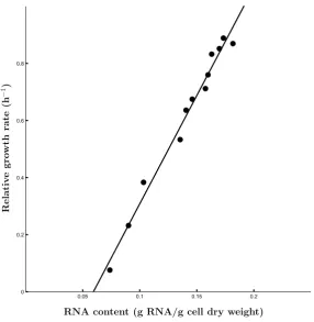
2.2 Relationship between relative growth rate and RNA content . . . 34

2.3 Graphical reconstruction of the functionr1(·) . . . 36

2.4 Empirical laws . . . 38

2.5 Numerical solution of the system withn=1 . . . 39

2.6 Stationary cycle under a sinusoidal variation ofψ1 . . . 40

3.1 Schematic representation of the model for the casen=2 . . . 68

3.2 Numerical solutions of the PWS system forn=1 . . . 77

3.3 Numerical solutions of the PWS system forn=1 with its space regularisation . . . 81

4.1 Reconstruction of ther-function forEscherichia coligrown under carbon-limited conditions 91 4.2 Reconstruction of ther-function for Scenedesmus sp.grown under phosphorus-limited condition . . . 92

4.3 Reconstruction of ther-function forSkeletonema costatumgrown under nitrogen-limited conditions . . . 94

4.4 The time-varying environment of the ‘feast-or-famine’ type . . . 97

4.5 Fitness-optimal mid-point shape parameter of the regulatory function as a function of the environmental parameter . . . 98

4.6 Fitness-optimal steepness parameter of the regulatory function as a function of the envi-ronmental parameter . . . 99

4.7 Stationary cycles for fitness-optimalr-functions . . . 100

5.1 Glucose-lactose diauxic growth ofE. coli . . . 125

5.2 Diauxic growth . . . 126

(6)

List of Tables

2.1 Notation employed in the equations describing the model . . . 27 2.2 Assumptions used in the analysis of the model . . . 28 4.1 Assignment of major classes of proteins, grouped according to function, to macro-chemical

(7)

Abbreviations

ATP Adenosine-50-triphosphate CAC Citric acid cycle

CoA Co-enzyme A

DNA Deoxyribonucleic acid

Fts Filamentous temperature sensitive

NAD+ Oxidized form of nicotinamide adenine dinucleotide NADH Reduced form of nicotinamide adenine dinucleotide

NADP+ Oxidized form of nicotinamide adenine dinucleotide phosphate NADPH Reduced form of nicotinamide adenine dinucleotide phosphate ODE Ordinary differential equation

PE Phosphorylation equivalents PMF Proton-motive force PWS Piecewise smooth RE Reducing equivalents Redox Reduction-oxidation RNA Ribonucleic acid

(8)

Acknowledgements

I am deeply grateful to my supervisor Dr Hugo van den Berg. I am indebted to him for his intellectual support, scientific professionalism, as well as his patience and belief in my potential. His invaluable advise and help with content, style, illustrations, and English made it possible for me to complete this thesis. I will always admire him as a great scientist, an inspiring mentor, a talented human being, and a sincere person.

I am warmly thankful to my husband, who comforted and inspired me in moments of despair, and who never doubted in my capacities. His support always motivated me to keep moving.

I am obliged to my brother for his contribution to Chapter 4 as a software developer. His cooperation and support helped me to complete the thesis earlier.

(9)

Declaration

This thesis by published work is submitted to the University of Warwick in support of my application for the degree of Doctor of Philosophy. It has been composed by myself and has not been submitted in any previous application for any degree.

The work presented was carried out by the author, with the following exceptions: the theory was devel-oped and interpreted in discussions with the supervisor; theMathematicacode for simulations carried out in Chapter 4 was translated into theJavacoding language by software developer Oleg A. Nev, but the simulations were subsequently ran by myself; artwork pertaining to micro-organisms was kindly pro-vided by the supervisor. Furthermore, Chapters 2– 4 were published as papers and as such benefited from the comments and suggestions provided by anonymous referees.

Chapter 2 was published as:

Nev O. A. and van den Berg H. A. (2017) Variable-Internal-Stores models of microbial growth and metabolism with dynamic allocation of cellular resources.J. Math. Biol., 74 (1), 409–445.

Chapter 3 was published as:

Nev O. A. and van den Berg H. A. (2017) Differential inclusions with sliding modes to represent microbial metabolism and growth under conditions of starvation.Dyn. Systems, doi: 10.1080/14689367.2017.1298726. Chapter 4 was published as:

(10)

Abstract

(11)

Chapter 1

Introduction

This thesis describes the development of a macro-chemical kinetics model of metabolism and growth in micro-organisms that allows the integration of observations on metabolic regulation and nutrient dis-position with data regarding the ambient conditions to which the organisms are subjected. The model focuses on the rates of exchange of matter and energy between micro-organisms and their environment, with a view to applications in both fundamental ecology and biotechnology, for instance in assessing the contribution made by microbiota to mass and energy fluxes in ecosystem. This introductory chapter will motivate the development of such models. Section 1.1 describes the basic biology of both prokaryotic and eukaryotic micro-organisms. Section 1.2 discusses standard culture systems. Section 1.3 reviews mod-elling strategies, ranging from the most minimal models to biochemically detailed models and explains where the modelling philosophy adopted in the present thesis lies within this range.

1.1 General microbiology

This section describes the basic principles of the biology of both prokaryotic and eukaryotic cells that underpin the model developed in this thesis.

1.1.1 Prokaryotes

This section focuses on prokaryotic micro-organisms and their structural and physiological traits, classi-fying intracellular components according to the macro-chemical concept proposed in this thesis.

Structural components and nutrient uptake apparatus

(12)

en-Figure 1.1: Structure of a phospholipid bilayer. Lipid molecules form a bilayer in such way that hydrophobic ‘tails’ are isolated from the surrounding aqueous environment, while the hydrophilic ‘heads’ interact with this envi-ronment. The membrane contains numerous proteins which may span the membrane, or be attached or anchored to the membrane, depending on their type and function.

velope and the genetic material, as well as intermediates of core metabolic pathways. In addition, we discuss transporters and binding proteins involved in the assimilation of nutrients from the environment; in the conceptual scheme of the present thesis, such proteins are grouped together asuptake machinery.

Cell envelope Prokarytotes are unicellular micro-organisms that are characterised by the absence of a true nucleus. They are among the most primitive and ancient known forms of life [48]. The cytoplasm of prokaryotic cells is enclosed by a bilipid membrane, the schematic structure of which is shown in Fig. 1.1. The cytoplasmic membrane is a phospholipid bilayer in which various proteins are embedded. Within this bilayer, the fatty acid tails of the constituent lipid molecules point inward, toward each other, thereby forming a hydrophobic region [98]. Membrane proteins perform various biological activities, such as cell-to-cell interaction, signalling, or transporting substances across the membrane. Certain membrane proteins called integral membrane proteins are partly or fully embedded in the membrane or span it [97]. There are also peripheral proteins which are not embedded in the cytoplasmic membrane, but firmly associated with its surface (Fig. 1.1).

Depending on the reaction of the cell to the Gram stain, bacterial species are classified as either Gram-positive or Gram-negative [58]. In Gram-Gram-positive cells a rigid polysaccharide layer called peptidoglycan forms 90% of the cell wall, whereas in Gram-negative bacteria the peptidoglycan layer is very thin, and there is a second bilipid membrane called the outer membrane, which consists of phospholipids, proteins, and polysaccharides [109]. The area between outer and cytoplasmic membranes is filled by a special layer with a high protein concentration, which is called the periplasm [55]. The main structural differences of the cell wall between Gram-positive and Gram-negative bacteria are shown in Fig. 1.2.

(13)

Outer membrane Periplasmic space

Peptidoglycan

Cell membrane

Cytosol

��

Figure 1: cc.

Figure 1.2: Comparison of the cell wall in Gram-positive and Gram-negative bacteria.Both Gram-positive (left)

and Gram-negative (right) bacteria have a cell membrane enclosing the cytosol, with a peptidoglycan (murein) layer covering the external surface of the cell membrane. Whereas this peptidoglycan is thick in Gram-positive bacteria, it is quite thin in Gram-negative bacteria. However, in the latter, the cell envelope is completed by an additional outer membrane, which forms a periplasmic space between the outer and inner membranes.

provides the cell with a form of energy storage called proton-motive force (PMF), which drives transport and motility functions of the cell [98].

(14)

[image:14.595.115.518.82.241.2]

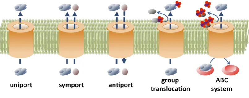
Figure 1.3: Modes of transport.

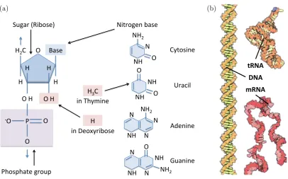
Genetic material Genetic information required for growth, development, metabolism, and reproduction is stored in the form of the deoxyribonucleic acid (DNA). The latter is composed of a sugar-phosphate backbone, with a nitrogen-rich organic base attached to each sugar moiety (Fig. 1.4). There are 4 bases (adenine, thymine, cytosine, and guanine), which serve as the ‘alphabet’ used to encode information. For instance, to encode one of the 22 amino acids that occur in microbial proteins, a three-base ‘word’ (codon, triplet) is used (there are 43₌_{64 such ‘words’). To encode the entire protein, the requisite number of}

codons is concatenated into a functional unit called the cistron. One or several cistrons under the control of a single upstream activating region (promoter, operator) make up an operon. Having several proteins under common control often makes functional sense, for instance if they are enzymes pertaining to a particular biochemical pathway. Promoter and cistron(s) together constitute a gene. Several hundreds to many thousands of genes make up the genome of a given micro-organism [9].

Bacterial cells typically have a single circular chromosome [143], which is folded into a structure termed the nucleoid [144]. In addition to the large DNA molecule, bacteria may contain small loops of DNA called plasmids, which can be transferred between bacterial cells [55].

Synthetic machinery

This section describes the molecular machinery of a cell that is devoted to the synthesis of catalytic machinery via the processes of transcription and translation. This type of machinery will be referred to assynthetic machineryin this thesis.

(15)

syn-O" Base" H" H" O"H" H" H" H2С"

P" O" O" !_O" Sugar"(Ribose)" Nitrogen"base" Phosphate"group" N" NH" O" NH2"

Cytosine" NH" NH" O" O" Uracil" in"Thymine" N" N" NH2"

NH" N" Adenine" NH" N" NH" N" Guanine" O"

NH2"

O"H"

in"Deoxyribose" H" H3C"

(a)

DNA$ tRNA$

mRNA$

[image:15.595.113.520.71.324.2]

(b)

Figure 1.4: Nucleic acids: RNA and DNA. (a)Structure of RNA. In DNA, the sugar deoxyribose is present instead

of ribose, and the nitrogen base thymine replaces uracil.(b)Double-stranded helix molecule of DNA together with

the molecules of messenger and transport RNAs (taken from [55]).

thetic apparatus [55]. Figure 1.4 illustrates key differences between DNA and RNA. DNA has the sugar deoxyribose in its backbone, whereas RNA has the sugar ribose. Furthermore, the nucleotide thymine in DNA is replaced by uracil in RNA. Three major types of RNA molecules are messenger RNA (mRNA), transfer RNA (tRNA), and ribosomal RNA (rRNA).

(16)

9/:;+<!

9/:;=<! 7'/;+<!

7'/;=<!

&#(/.0#1"2$/!

&#(/.,(2$/!

&#(/.0#1"2$/!

&#(/.,(2$/!

+!

>!

=!

(a)

!"#$%&'"()*#+& +#,+#--.+& !"#"$#"%%&'()

!,.-%&'"()*#+& /*01/2.+& &(!*+,'() 3&

*.+#,+#--.+& +#,+#--.+& #"$#"%%&'()

'"4'5'2.+& /*01/2.+& &(-+,.-,'()

3&

(b)

Figure 1.5: Regulatory mechanisms in bacteria. (a)Diagram illustrating modes of control in prokaryotic gene

regulation. Two alternative substrates (AandB) are both converted to a common product (P), via reactions catalysed

by specific enzymes (enz(A) andenz(B)) which are encoded by genes (gen(A) andgen(B)). In negative feedback

control, the expression of both these genes is inhibited by productP. In positive feedforward control, the expression of the gene corresponding to the enzyme converting a given substrate is stimulated by that same substrate, whereas in negative feedforward control, the expression of the gene corresponding to the enzyme converting a given substrate is inhibited by the alternate substrate. These various modes can co-exist together, mediated via several regions upstream from the promoter, where activating and repressing proteins can interact with the DNA and thus modify the

rate of assembly of the RNA polymerase at the promotor.(b)Modes of regulation of gene expression. Stimulation

of the expression of a given gene can be mediated by activation, in which an activator protein interacts with the upstream regulating region of the gene; this involves interaction with an inducer. Stimulation may also be effected via derepression, in which a repressor (an inhibitory transcription factor) is rendered less effective by an inducer. Inhibition of gene expression can likewise be achieved in two ways, either via inactivation of the activator protein via interaction with an inhibitor, or via activation of the repressor by binding to a corepressor. Inducers, inhibitors, and corepressors are frequently metabolities (substrates or products) but can also be components of an intracellular signalling cascade.

is released from the ribosome. The process stops when the so-called stop codon is reached, after which the polypeptide chain is released by the ribosome and is folded into an active protein [98].

Regulatory mechanisms In order to thrive, micro-organisms have to be able to respond rapidly to changes in the environment. One of the ways in which they can do this is adjusting gene expression. Cells regulate their uptake machinery both qualitatively and quantitatively in order to conserve energy and resources. This regulation is performed by the cell either via activity control or via amount control, or via a combination of these two modes. Activity can be adjusted only after the completion of protein synthesis, whereas the amount is regulated at a level of either transcription or translation [42].

(17)

core-(a) (b)

Figure 1.6: Examples of regulatory mechanisms in bacteria. (a)Transcription of the maltose transport system

gene is initiated via the induction regulatory mechanism, in which the inducer binds the maltose activatory protein,

which binds the RNA polymerase and thus makes it starting transcription.(b)Transcription of the arginine

biosyn-thetic pathway gene is blocked via the repression regulatory mechanism, in which the corepressor binds the arginine repressor, thus makes it active and lets it stopping transcription.

pressor binds to the corresponding regulatory protein called the repressor, which subsequently changes its conformation and blocks transcription. The example of repression of transcription of the arginine biosyn-thetic pathway gene is shown in Fig. 1.6 (b). In inactivation, an inhibitor binds to a regulatory protein called the activator, and thus inhibits its activation and, subsequently, transcription. In positive control, an enzyme is produced only if the substance, whose synthesis is catalysed by this enzyme, is present. This type of regulation can be operated either via induction or via derepression. The former is carried out by a specific protein called the activator that activates the binding of RNA polymerase to DNA, as follows: the so-called inducer binds to the activator protein which interacts with the DNA at an activator-binding site and allows RNA polymerase to begin transcription [27, 92]. The example of induction of transcription of the maltose transport system gene is shown in Fig. 1.6 (a). In derepression, the inducer binds to the repressor and thus stops the repression of transcription.

There are additional modes of regulation which come into play under conditions of extreme stress. Nutrient shortage in the environment induces an increase in a number of uncharged tRNAs in a cell, and as the number of uncharged tRNA relative to the number of charged tRNA grows, the ribosome wastes a greater portion of its time interacting with uncharged tRNA, which thus leads to a stall of the ribosome along with a production of small nucleotides called alarmones. The alarmones initiate the so-called stringent response that is characterised by a cessation of rRNA and tRNA synthesis and ribosome production as well as by a decrease in protein and DNA synthesis and amino acid production [24, 109].

(18)

Figure 1.7: Schematic representation of a cell division process.First, DNA is replicated and the cell is elongated. Then new materials are generated and new DNAs are divided. Finally, two daughter cells are formed.

helping the cell to recover from heat stress [167]. The same regulatory mechanism is used to withstand critical conditions caused by chemicals or radiation.

Growth machinery

In this section we review processes related to cellular growth, which are mediated by thegrowth machin-erythat synthesises the cell envelope and mediates genome duplication and cell division. In addition, the growth machinery shares the molecular apparatus with the synthetic machinery to generate novel structural components.

Cell division The process during which an increase in the number of cells is observed can be defined as microbial growth [98]. This process involves a large complex of different chemical reactions occurring in a cell, such as energy transformation reactions, monomer synthesis reactions, and polymerization re-actions, in which monomers are joined together to form macromolecules. A schematic representation of this process is given in Fig. 1.7.

(19)

membrane are subsequently synthesised, and the two chromosomes are pulled apart. Then the ring that was formed by Fts proteins depolymerises, and a special partition called a septum is formed from the ring materials. Finally, the septum divides the cell in two approximately equal parts [28, 39, 146].

Growth rate The time required to produce one generation is called the generation time. This time depends on environmental conditions as well as on genetic traits of cells. If the number of cells doubles during a constant interval of time, growth is said to be exponential.

The relationship between the initial number of cells and their number after a period of exponential growth can be expressed mathematically by the formulaN=N02n, whereN0andNdenote, respectively,

the initial and final number of cells, andnis the number of new generations that occurred during the considered period of time. The generation timegcan be calculated ast/n, wheretis duration of growth. IfW is the biomass of the population, then ˙W _≡dW/dt is its growth rate and ˙W/W is the so-called specific growth rate, which characterises the growth rate relative to the size of the population. Since exponential growth is characterised by a constant specific growth rate, we have ˙W/W =const =µ,

whenceW(t) =W(0)eµt_{. Since} _N_/_N0₌_W_/_W0_{, we have 2}n₌_eµt ₌_eµng_{, whence we find that the}

doubling timegequals(ln 2)/µ.

Reserve components

In this section we review the components of a bacterial cell that underlie the storage of nutrients and which are mobilised to supply the central pools of core metabolites. In this thesis these components are usually calledreserves.

Bacterial cells form the main chemical compounds that are essential for growth from the nutrients that are assimilated from the environment. About 50% d/w of a typical cell consists of carbon, which is a major element in all macromolecules in a cell. Nitrogen comprises about 12% d/w of a bacterial cell, and is a key element in proteins and nucleic acids. Other essential elements, such as phosphorus, sulfur, potassium, magnesium, and calcium are present in smaller amounts [109].

(20)

a b _c

d

e f

Figure 1: cc.

Figure 1.8: A variety of reserve inclusions in prokaryotes.Depicted are inclusions of (a): cyanophycin,Anabaena

variabilis[168]; (b): sulfur, Thermoanaerobacter sulfurigignens[93]; (c): glycogen, Methylacidiphilum fumari-olicum[80]; (d): polyphosphate,Campylobacter jejuni[50]; (e): polyhydroxybutyrate,Rhodovibrio sodomensis[98];

(f): triacylglycerol,Rhodococcus opacus[3].

Metabolism of prokaryotes

The chemical transformations within a cell that are required to maintain all essential processes for its life are collectively called metabolism [98]. The core pathways of a bacterial metabolism are schematically presented in Fig. 1.9.

To be able to drive cellular processes and to grow, micro-organisms have to process the nutrients assimilated from the environment to provide the cell with energy that is required to drive metabolism and to furnish the building blocks for the macromolecules; cells also have to remove waste products from the cell. Metabolic reactions are typically divided into two categories: catabolic reactions that involve the breaking down of organic substances, and accordingly release energy, and anabolic reactions that help to create cellular components, and therefore consume energy [98].

(21)

A"&"G"

DNA"&"RNA"

C"&"T"

glycogen"

glucose" G6P"

G3P" 3PG" glycerol"

triacylglycerols" phospholipids"

fa>y"acids"

citrate"

2@oxo@glutarate"

heme," cyto@" chomes"

fumarate" oxaloacetate"

S"

A"

G"

F"

Y"

W"

H" V"

I"

L"

N"

D"

R"

T"

K"

M" C"

P"

Q"

[image:21.595.113.518.77.302.2]

E"

Figure 1.9: Core metabolism ofEscherichia coli. Atoms are presented as follows: black for C, white for H, red

for O, and purple for P. The main pathways are denoted by arrows: single-headed arrows for irreversible paths, and double-headed arrows for reversible paths. Single letter in circles indicate nucleotides. Single letters in squares

indicate amino acids. Other denotions are as follows: G6Pfor glucose-6-phosphate,PRPP for

phosphoribosyl-bisphosphate,Chorfor chorismate, G3P for glyceraldehyde-3-phosphate,3PG for 3-phosphoglycerate, Pyrfor

pyruvate,AcCoAfor acetyl-coenzyme A, andglyxfor glyoxylate.

constantly turning over, produced via catabolic reactions and consumed via anabolic reactions [98]. Fermentation and respiration are two modes of regeneration of ATP. Both start from the break down of glucose in glycolysis, which consists of the three following steps: the first stage of preparatory reactions that lead to production of two three-carbon sugar phosphates (glyceraldehyde-3-phosphate); the second phase, where energy is released and conserved in the form of ATP and two molecules of pyruvate are formed; and the last step, in which the fermentation products ethanol and CO2(or lactate) are formed [21].

The redox reactions that occur during this process take place in the absence of a terminal electron acceptor. If oxygen or another terminal acceptor is present (e.g. an inorganic compound), it is not necessary to synthesise the fermentation products, since glucose can be oxidized completely to CO2leading to the

increased production of ATP via the PMF. Thus in this case respiration process takes place, whose early two stages are the same as those of glycolysis, but the last stage occurs in the form of the pathway called a citric acid cycle (CAC), in which pyruvate is completely oxidizied to CO2.

1.1.2 Eukaryotes

(22)

prokary-Figure 1.10: Differences between prokaryotic and eukaryotic cells.TheEscherichia colicell is much smaller than the typical eukaryotic cell, where membrane-bound organelles, such as chloroplast and mitochondria, are present. The nucleus of eukaryotes contains several chromosomes and is separated from the cytoplasm by an envelope. In addition, prokaryotes lack certain membranous structures, such as the Golgi apparatus, vacuoles, and the endoplasmic reticulum, which are present in eukaryotic cells.

otic and eukaryotic cells is that the latter contain membrane-bound cellular organelles that are not present in prokaryotic cells, most notably the nucleus, the endoplasmic reticulum, and the Golgi apparatus [55]. Moreover, prokaryotes lack a nucleolus, a subcellular structure that is involved in the synthesis of ribo-somes [115]. The nuclear region in a typical prokaryotic cell contains a single chromosome that is not enveloped by a nuclear membrane, whereas in a standard eukaryotic cell it accommodates more than one chromosome and is surrounded by a double membrane layer that is contiguous with the endoplasmic reticulum. Another striking difference is the presence of mitochondria and chloroplasts in eukaryotes, organelles that have much in common with prokaryotic cells and be regarded as the descendants of en-dosymbiontic (cyano)bacteria [55]. Finally, the cell envelope in prokaryotic cells is more complex, both chemically and structurally, than in eukaryotic cells [85].

(23)

[image:23.595.110.524.72.263.2]

Figure 1.11: Four organisms investigated in this thesis: (a)the Gram-negative bacteriumEscherichia coli[109],

(b)the diatomSkeletonema costatum[1],(c)the haptophytePavlova lutheri[1],(d)the chlorophyteScenedesmus

sp.[1]

1.2 Standard culture systems

There are various ways of cultivating micro-organisms in bioreactors. The main methods of cultivation are batch cultivation and chemostat cultivation. There are several variations on these two types; examples include fed-batch cultivation or continuous cultivation with biomass retention [161].

1.2.1 Batch culture system

(24)

10 50 100 1

10

L

o

g

ce

ll

co

nce

n

tr

a

ti

o

n

(g

/

L

)

Time (h) Lag phase

Log phase

[image:24.595.175.460.71.357.2]

Stationary phase

Figure 1.12: Growth cycle for bacterial cells in the batch culture.Trichoderma reeseidata taken from [96].

The biomass-specific substrate consumption rate per unit of biomass of the populationqs _{mol W h}mol N

in the batch culture can be described as a function of the nutrient concentration[N] mol N

L

by means of the Michaelis-Menten equation [104]:

qs=qs,max

[N]

Km+ [N]

, (1.1)

whereqs,max mol W hmol N

represents the maximum substrate consumption rate, andKm mol NL

is the Michaelis-Menten constant, which denotes the concentration of the substrate at the half-maximal consumption rate [153]. Equation (1.1) can be derived by investigating the kinetics of an enzymatic reaction mecha-nism, i. e. by relating a reaction ratevto the concentration of a substrate[S]. The mathematical model of such reaction proposed by L. Michaelis and M. Menten [104] can be schematically presented as follows:

E+S

kfor

krev

(25)

and catalytic reaction rate constants. Sinced[ES]/dt=0, we have:

kfor[E][S]−krev[ES]−kcat[ES] =0,

hence

[E] =Km

[ES]

[S] withKm=

krev+kcat kfor

.

The reaction ratevequals tod[P]/dt=kcat[ES], and thus we obtain: v= vmax

1+Km/[S]

withvmax=kcat[E0],

where[E0] = [E] + [ES] = [ES](1+Km/[S])is the initial (free) enzyme concentration. Replacingvwithqs

and[S]with[N], we obtain eqn (1.1).

In a general case, where the cooperativity between different binding sites of the same enzyme is taken into account, eqn (1.1) can be extended to the Hill equation [70]:

qs=qs,max

[N]n

Kn m+ [N]n

, (1.3)

wherenis the Hill coefficient that describes the degree of interaction (cooperativity) between different binding sites of the same enzyme. The Hill coefficientn=1 will be used throughout this thesis for the sake of simplicity. Whereasn=1 has been confirmed for numerous systems (e.g. [41, 123]), the case

n>1 may be appropriate for certain uptake systems (e.g. [91]); however, the general principles of the dynamic reallocation theory carry through provided the functional response is monotonically increasing. The Pirt equation [118] describes the relation betweenqsand the specific growth rateµ(1/h)during

the exponential phase:

qs=µ/Ys,max+ms, (1.4)

whereYs,max mol W_{mol N}

is the maximum yield of biomass, andms _{mol W h}mol N

is a maintenance coefficient, which shows the biomass-specific rate of substrate consumption to maintain activities performed by the micro-organism in the absence of growth. Sinceµ=W˙/W, whereW is the biomass of the population

and the dot indicates the differentiation in respect to time (cf. Section 1.1.1), we have: ˙

(26)

Figure 1.13: The chemostat. The main vessel contains a well-stirred culture medium, which is replenished from the reservoir. The culture vessel maintains a constant volume of culture, since the inflow of a fresh medium from the reservoir equals the outflow of a spent medium (overflow) from the vessel.

and together with eqn (1.1) this yields: ˙

W =Ys,max

qs,max

[N]

Km+ [N]−

ms

W. (1.5) The following conservation law applies if intracellular reserves do not vary:

[N]0= [N] +W/(Ys,maxV) +ms/V

Z τ

0

W(τ)dτ, (1.6)

where[N]0 mol N_L expresses the initial nutrient concentration andV(L)is the volume of the medium in

which the culture is grown. This allows us to obtain a system of differential equations forW and[N].

1.2.2 Chemostat culture system

For many studies it is advantageous if cultures can be maintained in constant environmental conditions for long periods, which is not possible with closed cultures of the batch type, since the culture is always undergoing dynamical change in the latter type of culture. However, such steady-state conditions can be achieved in a continuous-flow culture, or chemostat (Fig. 1.13). The cultivation in the chemostat is characterised by a continuous supply of fresh medium and withdrawal of an equal volume of cultivation broth, which allows the cultivation volume to remain constant [37]. After a certain time the system reaches a state in which the chemostat volume, the cell number, and the nutrient status remain constant; the system is then said to be in steady state.

(27)

si-multaneously. To provide such control, the experimenter can manipulate two key parameters: the first parameter is dilution rateD=F/V(1/h), whereV(L)is the volume of the main vessel, andF(L/h)is the flux at which fresh medium is pumped in, and spent medium is removed from, the chemostat; and the second parameter is the concentration of limiting nutrients[N]R(mol N/L)in the reservoir. Varying the

dilution rate, different growth rates can be achieved.

The balance equation for biomass concentration[W] (mol W/L)in the chemostat of volumeV is as follows:

d(V[W])

dt =µV[W]−F[W], (1.7)

whereµis a biomass-specific growth rate [153]. Since the vessel volumeV remains constant in time, we

have:

d[W]

dt =µ[W]− F

V[W]. (1.8)

The balance equation for nutrient concentration[N]in the main vessel is as follows:

d[N]

dt = F

V([N]R−[N])−σeWµ[W], (1.9)

where[N]R is the nutrient concentration in the reservoir, and σeW(mol N/mol W) is a stoichiometric

coefficient [153]. At steady state, the concentration of biomass[W]and the concentration of nutrient in the culture vessel[N]do not change in time, so thatd[W]/dt=0, andd[N]/dt=0. Hence we obtain the following steady-state chemostat equations:

µ=D; [N] = [N]R−σeW[W], (1.10)

whereD=F/V– dilution rate. The first equation shows that by setting the dilution rateDof the chemo-stat to a certain value, we are able to cultivate micro-organisms at specific growth rate equal toD, which makes the chemostat an important laboratory tool to study the physiology of microbes under well-defined conditions (constant growth rate, constant environmental conditions) or to examine how the growth rate affects, for instance, the rate of product formation. Figure 1.14 shows how bacterial concentration[W], bacterial yieldY, doubling timeg, and nutrient concentration[N]depend on the dilution rate at the steady state in the chemostat [130]. Calculations based on the steady-state chemostat eqns (1.10) together with the Monod equationµ([N]) =µb(1+KS/[N])−1[107] (which was originally proposed as a purely

(28)

0.2 0.4 0.6 0.8 1 0

1 2 3 4

5 Bacterial concentration (g/l)

Doubling time (h) Bacterial yield (g/l⇥h 1₎

Nutrient concentration (g/l)

[image:28.595.194.439.71.331.2]

Dilution rate (h 1₎

Figure 1.14: Steady-state relationships in the chemostat. Relationship between bacterial concentration,

bacte-rial yield, doubling time, and nutrient concentration in the steady state depending on different dilution rates in the chemostat described by eqns (1.11) with parametersµb=1 h−1,KS=0.2 g/l,σeW=1,[N]R=10 g/l.

is the nutrient concentration at whichµ=0.5µb) yield the following expressions which describe these

relationships:

[W] =

[N]R−

DKS

b

µ−D

e

σ_W−1;

g= (ln 2)/D;

Y =D

[N]R−

DKS

b

µ−D

e

σ_W−1;

[N] = DKS

b

µ−D.

(1.11)

(29)

1.3 Mathematical models of microbial growth

Models of bacterial growth can be in general written as ˙

W =µ(x,u)W , (1.12) whereW_∈R+is a suitable measure of biomass,x∈Rprepresents the internal state,u∈Rqrepresents

external conditions that affect growth and metabolism,µis a functionRp+q7→R+, called themodel, and

the dot indicates differentiation with respect to time [24]. Here,W,x, anduare all allowed in general to be functions of timet. Classic models tend to be characterised by p=0 orp=1 (i. e. they have little or no structuring in terms of the internal state), whereas detailed ‘system biology’ or ‘in silico’ models can have very largep, on the order of hundreds or thousands [38].

1.3.1 Classic macroscopic models

Models are specified by the choice of the functionµ:Rp+q7→R+. For instance, the Monod model is as

follows:

µ([N]) =µb(1+KS/[N])−1, (1.13)

where[N]is the ambient concentration of the limiting nutrient andbµandKSare positive parameters [107].

As Monod pointed out [107], the parameterKSshould not be confused with the parameterKmin eqn (1.1).

In terms of our general description, eqn (1.12),p=0 andq=1: there are no state variables other thanW

and there is a single environmental variable,[N], on which the specific growth rateµdepends. If we allow [N]to vary in time, we haveW(t) =W0expR0tµ([N](τ))dτ . One way to extend this model toq>1,

but still withp=0, is to posit a multiplicative formµ(u1,u2, . . .) =µbf1(u1)f2(u2)···[26, 56], where the

u1,u2, . . .are relevant environmental factors (such as levels of light, nutrients, and redox substrates) and

the f1,f2, . . .are appropriate functions_R+_7→[0,1]that express how these factors affect growth.

Another approach is used by Pirt [74, 118], who proposed eqn (1.4) to describe the relationship between the the specific growth rateµand consumption rateqsof the substrate used as an energy source.

A related concept known as an ‘endogenous metabolism’ was introduced by Herbert [67] to study the dependence between the growth yield and the growth rate:

˙

(30)

where the termaW is the expenditure of the organism for the ‘endogenous metabolism’, which is es-sentially equal to the maintenance energy. This idea was further developed by Marr et al. [100] in the following equation, proposed as an empirical description for continuous culture (chemostat) data:

1

W = a Wmax

1

D+

1

Wmax , (1.15)

whereDis the dilution rate of the chemostat andWmaxcorresponds to the maximum possible biomass

concentration.

In the opposite situation, when growth is assumed to depend on the internal state of the micro-organism only, so that p=1 and q=0, we obtain another modelling subclass, whose most-studied member is perhaps the Droop equation [36]:

µ(Q) =µb(1−Q0/Q). (1.16)

Here,Qcharacterises the internal state of the cell, namely, the internal nutrient ‘pool’ called the cell quota, which comprises the particle species of interest in any of its biomolecular speciations (e.g. free molecules, part of polymers, machinery etc.). By definition, the cell quota is the intracellular density of the chemical element of interest (amount per cell), which can roughly be thought of as an average concentration [35]. The parameterQ0is the so-called ‘subsistence quota’, which can be interpreted as the minimum cell quota required by the cell to maintain its structural integrity. Growth at a non-zero rate requiresQ>Q0. A similar equation was proposed by Caperon [16] in the following form:

µ(q) =µbq(q+A)−1_, _(1.17)

whereqexpresses the reserve nutrient content of the cell, andAis the so-called growth kinetic constant, which Caperon identified withQ0[15]. In terms of the Droop model,q=Q₋Q0.

(31)

This journal isc _{The Royal Society of Chemistry 2013} Mol. BioSyst.,2013,9, 1576--1583 1577

The information contained in these extracellular signals is

decoded and translated by liver cellsviasignalling and

regula-tory processes.

Complex diseases are systemic phenomena aﬀecting

multi-ple cellular processes. For exammulti-ple, cancer is characterised by a deregulation of the mechanisms that govern transduction of extracellular signals into the gene expression system, but also

by an impaired functioning of its metabolic machinery.5_Hence,

only an integrated view of the processes involved can lead to a comprehensive understanding that may shed new light on the development of these diseases and, therefore, provide new treatment opportunities.

Mathematical modelling has become a key methodology for gaining a deeper understanding of complex biological

pheno-mena and for predicting phenotypes under diﬀerent conditions.

Similarly to what happens in experimental studies, signalling, gene expression, and metabolism are often modelled separately and integrated models are still scarce. Accordingly, mathematical form-alisms have been developed independently, tailored to the nature of the biochemical interactions and molecules involved, and to the

specific features of the processes in each domain. Some eﬀorts have

attempted to connect these diﬀerent processes, both experimentally

and computationally. Given the complexity of the task, studies in

this direction so far have been limited in number and scope.6

We believe that the time has come to address this challenge. The main motivation, in our opinion, is the rapid development

of high-throughput measurement techniques for these diﬀerent

types of data, associated with the corresponding ‘omics’ label: in

historical order, genomics, transcriptomics (gene expression), proteomics and metabolomics. While there are undoubtedly many challenges, modelling approaches that leverage these data,

as well as improved parameter optimisation algorithms7 _and

high-performance computing, should be a major avenue of research in the coming years in systems biology. This should lead to a broad range of potential applications in biotechnology, biomedicine, and pharmaceutical research.

In this review, after a brief summary of existing modelling approaches for signalling, metabolic, and gene regulatory processes,

we describe recent eﬀorts to connect these layers (Fig. 2).

Di

ﬀ

erent layers are modelled with di

ﬀ

erent

mathematical formalisms

All cellular processes, from the basic to the most complex, result from the interaction of a large number of biological molecules. On a structural basis, these interactions can be described as networks, usually as graphs or, more generally,

hypergraphs. Graphs are composed of nodes (e.g.proteins) that

are connectedviaedges, the latter representing some relationship

between pairs of nodes. Hypergraphs, additionally, facilitate the representation of relationships with more than two interacting

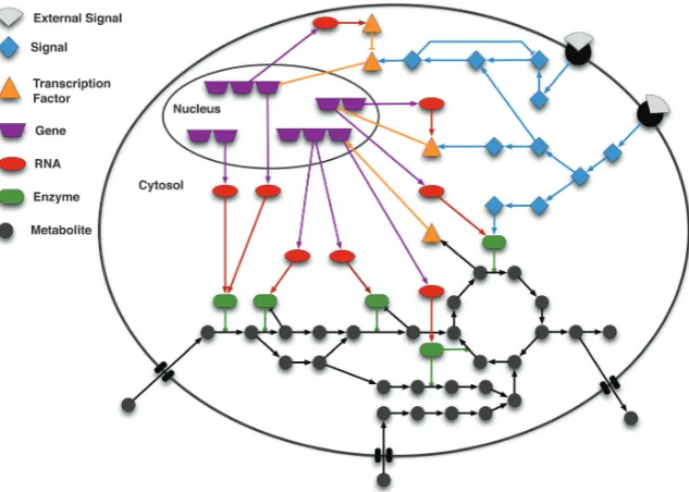
Fig. 1 Schematic of the interconnection among signalling, gene regulation and metabolism. In a cell, signalling networks are activated by external signals,e.g.

ligands (grey shapes) binding to a receptor (black semi-circles) located in the cell membrane. The signal is then internally propagated in the cell by means ofe.g.

protein phosphorylation cascades. These cascades may lead to alterations in the expression of genes by activating or inhibiting transcription factors (TFs). Gene regulatory networks control the transcriptional level of genes, and thus the production of messenger RNA molecules, which are subsequently translated into proteins. These proteins are in turn involved in cellular functions, including signal transduction and the catalysis of metabolic reactions. Specific metabolites are known to aﬀect proteins’ activity (e.g.binding to the allosteric site) and can also influence gene regulation. As illustrated in the scheme, signalling, gene regulation, and metabolism are tightly interconnected showing that the systems’ behaviour can only be accurately modelled and understood by properly integrating the sub-systems. The interactions between the molecules are represented by edges: arrow shaped edges represent activating interactions; blunt edges represent inhibitory interactions; and edges with a circle on the top end depict enzyme reaction catalyses.

Review Molecular BioSystems

Open Access Article. Published on 01 March 2013. Downloaded on 23/02/2017 11:25:57.

View Article Online

Figure 1.15:Schematic representation of signalling, gene regulation and metabolic network inside of the cell (taken

from [53]). Edges of the graph represent the interactions between the molecules. In particular, activating interactions are shown by arrow shaped edges; inhibitory interactions by blunt edges; and enzyme reaction catalyses are edges with a circle on the top end.

1.3.2 Microscopic models

Regarding models withp>1, one might decide to account explicitly for the position and movement of every molecule inside the cell (p_∼108) or at least for the concentrations of all molecular species. Mi-croscopic models in most of the cases are focused on specific subsystems of the cell describing either metabolism, gene expression, or signal transduction [53]. These models typically define cellular pro-cesses as interactions between a large number of biological molecules that can be described as networks by means of graphs with nodes connected via edges [83] as schematically shown in Fig. 1.15. Depending on the specific properties of the given biological network under consideration, different formalisms can be employed to simulate its dynamic behaviour.

[image:31.595.160.477.71.297.2]

(32)

regulation of metabolism in human red blood cells [121], whereas flux balance analysis has been used to investigate the yield-optimal behaviour ofEscherichia coliin dependence of oxygen availability [160]. Other techniques have been employed, for instance, to model the electron transport chain of mitochon-dria [5] or to describe the kinetics of the electron transport chain of purple non-sulfur bacteria [82].

The construction and analysis of models that are capable of describing the cell as a whole system is challenging. One good example is the model of central metabolism ofEscherichia coli, where the state variables are metabolite concentrations, gene expression levels, transcription factor activities, metabolic fluxes, and biomass concentration [38].

Although the micro-chemical approach seems to be straightforward, the models of this class typically have high-dimensional state spaces (i.e., a large number of dynamic degrees of freedom: the latter was represented in Section 1.3.1 byp) and substantial parametrization problems, and therefore may become unattractive due to their complexity.

1.3.3 Variable-Internal-Stores-with-reallocation model

The casesp=0 andp_∼108represent the opposite ends of a range, on which the modeller has to choose an optimal compromise in accordance with the available information and the purpose of the modelling exercise. Given that the dynamics of other intracellular compounds besides structural biomass is often physiologically relevant, this thesis will focus on models wherep₆=0. Our modelling strategy is to try to formulate models that (i) are sufficiently versatile to accommodate detailed information, particularly ‘big data’ such as transcriptomics, proteomics, and metabolomics, (ii) are consistent with basic principles such as conservation laws, (iii) remain relatively tractable, and, in particular, reduce to the simple classic models as special cases. Variable-Internal-Stores (VIS) models [35, 61, 165] fulfil these desiderata. The point of departure is to consider the dependence of the growth not only on nutrient influx from the envi-ronment, but also on reserve levels inside of the cell (cf. Section 1.1.1). Taking into account internal stores allows for an accurate description of the rates of resource consumption and bioproduction yields [24]. A basic example of the VIS model with a single internal variable store is the Droop cell quota model [35] discussed in Section 1.3.1.

(33)

of genes in response to changes in external conditions as well as in the status of internal availability of substrate [109], as discussed in Section 1.1.1, and changes in the gene expression profile are reflected in corresponding changes in the relative rates at which molecular building blocks are incorporated in molecular machinery [90].

The VIS-with-reallocation model achieves mathematical closure in the form of regulatory rules that drive this re-allocation. In this thesis, I show how these regulatory rules (r-functions) can be recon-structed by combining stoichiometric constraints with experimental observations of the behaviour of micro-organisms in response to changes in environmental conditions.

With such a model in hand, I investigate the question of adaptive microbial behaviour depending on ambient conditions, in particular, under nutrient shortage and time-varying environmental conditions.

1.4 Introduction to publications

This section previews subsequent chapters of this thesis that have been derived from peer-reviewed papers. Certain basic equations and figures in these chapters are repeated to render the individual chapters self-contained. Such equations and figures will be cited locally in each chapter.

Variable-Internal-Stores models of microbial growth and metabolism with dynamic allocation of

cellular resources

Variable-Internal-Stores models of microbial metabolism and growth have proven to be invaluable in accounting for changes in cellular composition as microbial cells adapt to varying conditions of nutrient availability. Here, such a model is extended with explicit allocation of molecular building blocks among various types of catalytic machinery. Such an extension allows a reconstruction of the regulatory rules employed by the cell as it adapts its physiology to changing environmental conditions. Moreover, the extension proposed here creates a link between classic models of microbial growth and analyses based on detailed transcriptomics and proteomics data sets. We ascertain the compatibility between the extended Variable-Internal-Stores model and the classic models, demonstrate its behaviour by means of simula-tions, and provide a detailed treatment of the uniqueness and the stability of its equilibrium point as a function of the availabilities of the various nutrients.

(34)

Microbial metabolism and growth under conditions of starvation modelled as the sliding mode of a

differential inclusion

We consider a model of bacterial growth with variable internal stores, extended with adaptive resource allocation and investigate the behaviour of this model under conditions of starvation, i.e. severe nutrient shortage, treating the behaviour under the starvation regime in terms of a differential inclusion and derive Filippov solutions. This Filippov sliding mode representation appears to be a simple but sound qualitative description of metabolic ‘shut down’ in response to starvation. We discuss a natural connection between biologically motivated modelling approaches to metabolic ‘shut down’ and numerical regularisation tech-niques to approximate Filippov solutions.

Full citation: Nev O. A. and van den Berg H. A. (2017) Differential inclusions with sliding modes to represent microbial metabolism and growth under conditions of starvation. Dyn. Systems. In press, doi: 10.1080/14689367.2017.1298726.

Optimal management of nutrient reserves in micro-organisms under time-varying environmental

conditions

Intracellular reserves are a conspicuous feature of many bacteria; such internal stores are often present in the form of inclusions in which polymeric storage compounds are accumulated. Such reserves tend to increase in times of plenty and be used up in times of scarcity. Mathematical models that describe the dynamical nature of reserve build-up and use are known as ‘cell quota,’ ‘dynamic energy/nutrient bud-get,’ or Variable-Internal-Stores models. Here we present a stoichiometrically consistent macro-chemical model that accounts for variable stores as well as adaptive allocation of building blocks to various types of catalytic machinery. The model posits feedback loops linking expression of assimilatory machinery to reserve density. The precise form of the ‘regulatory law’ at the heart of such a loop expresses how the cell manages internal stores. We demonstrate how this ‘regulatory law’ can be recovered from experimental data using several empirical data sets. We find that stores should be expected to be negiglibly small in stable growth-sustaining environments but prominent in environments characterised by marked fluctua-tions on time scales commensurate with the inherent dynamic time scale of the organismal system.

(35)

Chapter 2

Variable-Internal-Stores models of

microbial growth and metabolism with

dynamic allocation of cellular

resources

2.1 Introduction

Models of bacterial growth can be written as ˙W =µ(x,u)W, whereW _∈R+ is a suitable measure of

biomass,x_∈Rprepresents the internal state,u∈Rqrepresents external conditions that impinge on ˙W,

and the dot indicates differentiation with respect to time [24]. A basic model in this class specifies

µ([N]) =µb(1+KS/[N])−1, where[N]is the ambient concentration of the limiting nutrient andµbandKS

are positive parameters [107]. Here, p=0 and q=1: there are no state variables other thanW and there is a single environmental variable on which the specific growth rateµ depends. We allow [N]

to vary in time so thatW(t) =W0expR0tµ([N](τ))dτ . One way to extend this model toq>1, but

still withp=0, is to posit a multiplicative formµ(u1,u2, . . .) =bµf1(u1)f2(u2)_··· [26, 56], where the

u1,u2, . . . are salient environmental factors (such as levels of light, nutrients, redox substrates) and the

f1,f2, . . .are appropriate functionsR+7→[0,1]that express how these factors affect growth.

Regarding models withp>0, one might decide to account explicitly for the position and movement of every molecule inside the cell (p_∼108) or at least for the concentrations of all molecular species (p_∼

(36)

being produced, and this typically requires physiological structuring beyondp=0. Our point of departure is a class of models that lies at a mid-way point on this spectrum, withpsomewhere between 1 and a few dozen, known as Variable-Internal-Stores (VIS) models [35, 61, 165]. Taking into account internal stores, which in prokaryotes occur as metabolite pools, reserve compounds, and elemental inclusions [8, 109, 120], allows an accurate description of the rates of resource consumption and bioproduction yields [24].

In addition to VIS, we consider variations in the distribution of molecular building blocks among various types of molecular machinery [10, 152]. It is a priori likely that this allocation of building blocks is an important dynamic variable [95]; expression of genes is modulated, in prokaryotes as in eukaryotes, in response to changes in external conditions as well as in the status of internal availability of substrate [109], and changes in the gene expression profile are reflected in corresponding changes in the relative rates at which molecular building blocks are incorporated into molecular machinery [90]. Furthermore, in prokaryotes, the ability to adjust resource re-allocation among catalytic machinery has been shown to be an evolutionarily relevant trait, at least for certain kinds of ecological life history [156]. Finally, VIS-with-reallocation models should enable the reconstruction of regulatory rules that drive this re-allocation by combining stoichiometric constraints with observations of transient behaviour following changes in environmental conditions. For instance, in a continuous-culture system, such perturbations can be imposed by the experimenter and the response measured in terms of cellular composition, cellular density, as well as consumption and production of relevant chemical species (e.g. [26]).

The present paper describes the basic structure of VIS-with-reallocation models, taking care to dis-tinguish fundamental stoichiometric principles such as mass conservation from the constitutive relations that express these regulatory rules. We discuss the compatibility of this new class of models with well-established empirical laws in microbial growth and metabolism, as well as the observability of these constitutive relations. Moreover, we prove the uniqueness and stability of the equilibrium point under a reasonable assumption on the general appearance of the constitutive relations.

2.2 Variable-Internal-Stores with dynamic allocation theory

(37)

!

_&#

!

_"#

!

_$#

!

_'#

%

_$#

[image:37.595.112.527.384.779.2]

%

_'#

Figure 2.1: Schematic representation of the model described by the system (2.8) for the casen=2. Two types

of nutrients are assimilated by dedicated pathways (m1andm2) that feed into core metabolism from which building

blocks are sluiced to machinery synthesis (m0) and growth (mG). Core metabolism also exchanges molecular building

blocks with reserves (x1andx2).

assumptions are summarised in Table 2.2.

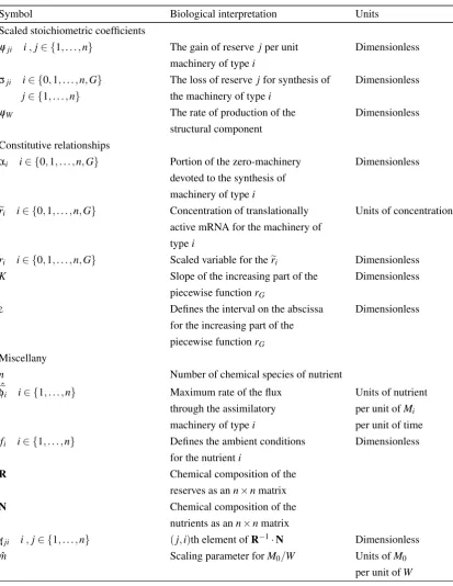
Table 2.1:Notation employed in the equations describing the model

Symbol Biological interpretation Units State unscaled variables

Mi i∈ {0,1, . . . ,n,G} C-molar amount ofi-type Moles of carbon

molecular machinery

Xj j∈ {1, . . . ,n} Molar amount of the primary Moles of the primary

elementXjin a reserve j element in a reserve

W C-molar amount of the structural Moles of carbon component

e

µ Specific growth rate Per unit of time State scaled variables

mi i∈ {0,1, . . . ,n,G} Density ofi-type molecular Dimensionless

machinery

xj j∈ {1, . . . ,n} Density of a reservej Dimensionless

µ Specific growth rate Dimensionless

Unscaled stoichiometric coefficients

e

φi i∈ {0,1, . . . ,n,G} The rate of production of the Units ofMiper unit

machinery of typei ofM0per unit of time e

ψji i,j∈ {1, . . . ,n} The gain of reserve jper unit Units ofXjper unit

machinery of typei ofMiper unit of time

e

σjW j∈ {1, . . . ,n} The loss of reserve jfor growth Units ofXjper unit

ofW e

σji i∈ {0,1, . . . ,n,G} The loss of reserve jfor synthesis Units ofXjper unit

j_{∈ {}1, . . . ,n_} of the machinery of typei ofMi

e

ψW The rate of production of the Units ofW per unit

(38)

Table 2.1:Notation employed in the equations describing the model

Symbol Biological interpretation Units Scaled stoichiometric coefficients

ψji i,j∈ {1, . . . ,n} The gain of reserve jper unit Dimensionless

machinery of typei

σji i∈ {0,1, . . . ,n,G} The loss of reserve jfor synthesis of Dimensionless

j_{∈ {}1, . . . ,n_} the machinery of typei

ψW The rate of production of the Dimensionless

structural component Constitutive relationships

αi i∈ {0,1, . . . ,n,G} Portion of the zero-machinery Dimensionless

devoted to the synthesis of machinery of typei

eri i∈ {0,1, . . . ,n,G} Concentration of translationally Units of concentration

active mRNA for the machinery of typei

ri i∈ {0,1, . . . ,n,G} Scaled variable for theeri Dimensionless

K Slope of the increasing part of the Dimensionless piecewise functionrG

ε Defines the interval on the abscissa Dimensionless

for the increasing part of the piecewise functionrG

Miscellany

n Number of chemical species of nutrient ˆ

e

φi i∈ {1, . . . ,n} Maximum rate of the flux Units of nutrient

through the assimilatory per unit ofMi

machinery of typei per unit of time

fi i∈ {1, . . . ,n} Defines the ambient conditions Dimensionless

for the nutrienti

R Chemical composition of the reserves as ann_×nmatrix

N Chemical composition of the nutrients as ann_×nmatrix

γji i,j∈ {1, . . . ,n} (j,i)th element ofR−1·N Dimensionless

ˆ

m Scaling parameter forM0/W Units ofM0

[image:38.595.109.523.89.624.2]

per unit ofW

Table 2.2:Assumptions used in the analysis of the model

Assumption Biological interpretation

σji=σjfor alli i,j∈ {1, . . . ,n} Amounts of reserves expended on the synthesis of different

types of machineries are the same

ψji=0 whenever j6=i i,j∈ {1, . . . ,n} The elemental ratios of the reserves are identical to the

elemental ratios of the nutrients

(39)

2.2.1 Stoichiometric equations

Basic definitions and dynamics

The bacterial cell is conceptually divided into several components, comprising molecular machinery, reserve compounds, and a structural component. The latter includes the cell envelope, genetic material, and core metabolites, small molecules that occur as intermediates of catabolic and anabolic pathways that are maintained at appropriate cellular concentrations by mechanisms not represented explicitly in the model. The C-molar amount of the structural component will be denoted asW.

Molecular machinery is divided inton+2 components, wherenis the number of chemical species of nutrient for which we wish to account (this choice is informed by available data as well as the envisaged application of the theory). Components 1 throughnrepresent the apparatus dedicated to the assimilation of the corresponding nutrients (transporters, binding proteins), in addition to the catalytic machinery that transforms these nutrients into core metabolites. Component 0 is the machinery required to synthesise machinery. Componentn+1, which will be given the subscript G, represents machinery devoted to growth, that is, the synthesis of the cell envelope and duplication of the genome. The C-molar amounts of thesen+2 types of machinery will be denoted asMi.

Reserve components correspond to storage of nutrients which is mobilised by the cell to replenish the central pools of core metabolites. We allow forndistinct types of such variable internal stores. Certain re-serves can be quantified in terms of C-moles, such as organic polymers such as poly-β-hydroxybutyrate, saccharides, as well as storage proteins, whereas others, such as sulphur globules and polyphosphate in-clusions that contain no carbon [120], are expressed in terms of molar amounts of the primary element Xj.

These Xj-molar amounts (where Xjis possibly but not necessarily C) will be denoted asXj.

Although machinery is a heterogeneous assembly of proteins, nucleic acids, and co-factors [109], it is nonetheless reasonable to assume that its chemical composition exhibits negligible fluctuations about the average typical of each kind of machinery. The dynamics of each component can then simply be written as follows:

˙

Mi=αiM0φei, (2.1)

wherei_{∈ {}0,1, . . . ,n,G_},αiis an allocation coefficient indicating which portion of the zero-machinery

is devoted to the synthesis of machinery of typei, andφeiis a stoichiometric coefficient. Parameters are

(40)

the model is rendered dimensionless. Being a fraction,αiis non-negative and subject to the constraint

∑

i∈{0,1,...,n,G}

αi=1. (2.2)

A unit of zero-machinery spends a fractionαiof its time producingi-type machinery. Thus, whenαi=1,

every unit of time,φeiunits of machinery of typeiare being produced per unit of zero-machinery. The

reserve components change according to the balance of uptake and expenditures [24]: ˙

Xj= n

∑

i=1 e

ψjiMi−σejWW˙ −M0

∑

i∈{0,1,...,n,G}

e

σjiαiφei, (2.3)

whereψeji is the gain of reserve jper unit machinery of typei,σejiis a stoichiometric coefficient for the

synthesis of machinery of typei, andσejW is a stoichiometric coefficient for growth. The last coefficient

can be further analysed into an assimilatory component, i.e. reserve jis used as building block, and a dissimilatory component, i.e.jis used as energy source; in general, reserve jmight be used in both ways andσ_ejW represents the net effect. Growth proceeds in proportion to the quantity of machinery that is

dedicated to it:

˙

W=ψeWMG, (2.4)

whereψeW is a stoichiometric coefficient. The specific growth rate equalsW−1W˙.

LetφbeifiMidenote the flux of nutrient molecules through assimilatory machinery of typei, whereφbeiis

a maximum rate andfi∈[0,1]depends on ambient conditions and possibly also on modulation by cellular

factors [30, 64]. Suppose thatE(1),E(2),. . .are the elements of interest. These could be any subset of the biogenic elements (C, H, O, N, S, P,. . . ) but in fact, any functional group or carbon skeleton that is not transformed by the metabolism of the organism of interest can be treated as an ‘element.’ For the sake of simplicity, we take the number of elements of interest to be equal to the number of reservesn. Nutrienti

has chemical formula (in its molecular form)Eν(11i),E (2)

ν2i E (3)

ν3i. . .E (n)

νni, where the subscriptνkiis the number

of elementkin a molecule of nutrienti. The chemical composition of the nutrients can be collected in ann_×nmatrixNwhoseith column is[ν1i,ν2i,ν3i, . . . ,νni]T. Similarly, the chemical composition of the

(41)

exists. Then we have _      n ∑ i=1e

ψ1iMi

.. .

n ∑ i=1e

ψniMi

    

=R

−1_N      b e

φ1f1M1

.. .

b e

φnfnMn

    , hence n

∑

i=1 e

ψjiMi= n

∑

i=1

γjiφbeifiMi,

whereγjidenotes the(j,i)th element ofR−1·N. We then have an explicit expression for the

stoichiomet-ric coefficientψeji:

e

ψji=γjiφbeifi. (2.5)

Scaling

Choosing suitable parameters as natural units, we may render the equations dimensionless, which can facilitate the analysis of a mathematical model [153]. Adoptingφe₀−1as unit of time, we define scaled

variables as follows:

mi=

Miφe0 Wm_bφei

; xj=

Xj

WσejW

. (2.6)

Herem_b is a scaling parameter forM0/W; its significance will be discussed in Section 2.2.2. Scaled

stoichiometric parameters are defined as follows:

ψji= e

ψjiφeimb

e

σjWφe02

; ψW= e

ψWφeGmb

e

φ₀2

; σji= e

σjiφeimb

e

σjWφe0

. (2.7) On this scaling, the specific growth rate(Wφe0)−1W˙ is equal to ψWmG; it is convenient to give this

quantity its own symbolµ. The biochemical similarity of different types of machinery implies that the relative amounts of reserves expended on their synthesis will be similar as well. This motivates the as-sumption that for every reserve j, we haveσji=σj for all machineries i. The scaled state variables

{m0, . . . ,mG,x1, . . . ,xn}represent densities: these are intensive variables, as opposed to the original

vari-ables_{M0, . . . ,MG,X1, . . . ,Xn}, which are extensive (i.e.,∝W). After scaling, we have the following

dynamics:

(

˙

mi =αim0−µmi fori∈ {0,1, . . . ,n,G}

˙

xj =∑ni=1ψjimi−µ(1+xj)−m0σj for j∈ {1, . . . ,n}.

(2.8) For the sake of simplicity, we shall assume henceforth thatψji=0 whenever j6=i. This is reasonable

Regulation of nutrient uptake, substrate conversion, and bio production in micro organisms

warwick.ac.uk/lib-publications

A Thesis Submitted for the Degree of PhD at the University of Warwick

Permanent WRAP URL:

http://wrap.warwick.ac.uk/98232

Copyright and reuse:

This thesis is made available online and is protected by original copyright.

Please scroll down to view the document itself.

Please refer to the repository record for this item for information to help you to cite it.

Our policy information is available from the repository home page.

Regulation of nutrient uptake, substrate conversion,

and bio-production in micro-organisms

Olga Alexandrovna Nev

Contents

List of Figures

List of Tables

Abbreviations

Acknowledgements

Declaration

Abstract

Chapter 1

Introduction

1.1

General microbiology

1.1.1

Prokaryotes

A"&"G"

C"&"T"

S"

A"

G"

F"

Y"

W"

H" V"

I"

L"

N"

D"

R"

T"

K"

M" C"

P"

Q"

E"

1.1.2

Eukaryotes

1.2

Standard culture systems

1.2.1

Batch culture system

1.2.2

Chemostat culture system

1.3

Mathematical models of microbial growth

1.3.1

Classic macroscopic models

Di

ﬀ

erent layers are modelled with di

ﬀ

erent

mathematical formalisms

1.3.2

Microscopic models

1.3.3

Variable-Internal-Stores-with-reallocation model

1.4

Introduction to publications

Chapter 2

Variable-Internal-Stores models of

microbial growth and metabolism with

dynamic allocation of cellular

resources

2.1

Introduction

2.2

Variable-Internal-Stores with dynamic allocation theory

!