Data mining of vehicle telemetry data

(1)

University of Warwick institutional repository:

http://go.warwick.ac.uk/wrap

A Thesis Submitted for the Degree of PhD at the University of Warwick

http://go.warwick.ac.uk/wrap/77645

This thesis is made available online and is protected by original copyright.

Please scroll down to view the document itself.

(2)

M A

E

G

NS I

T A T MOLEM

U N

IV

ER

SITAS WARWICEN SIS

Data Mining of Vehicle Telemetry Data

by

Phillip Taylor

A thesis submitted to The University of Warwick

in partial fulfilment of the requirements

for admission to the degree of

Doctor of Philosophy

Department of Computer Science

The University of Warwick

(3)

Abstract

Driving a safety critical task that requires a high level of attention and

work-load from the driver. Despite this, people often perform secondary tasks such

as eating or using a mobile phone, which increase workload levels and divert

cognitive and physical attention from the primary task of driving. As well as

these distractions, the driver may also be overloaded for other reasons, such as

dealing with an incident on the road or holding conversations in the car. One

solution to this distraction problem is to limit the functionality of in-car devices

while the driver is overloaded. This can take the form of withholding an

in-coming phone call or delaying the display of a non-urgent piece of information

about the vehicle.

In order to design and build these adaptions in the car, we must first have

an understanding of the driver’s current level of workload. Traditionally, driver

workload has been monitored using physiological sensors or camera systems

in the vehicle. However, physiological systems are often intrusive and camera

systems can be expensive and are unreliable in poor light conditions. It is

impor-tant, therefore, to use methods that are non-intrusive, inexpensive and robust,

such as sensors already installed on the car and accessible via the Controller

Area Network (CAN)-bus.

This thesis presents a data mining methodology for this problem, as well

as for others in domains with similar types of data, such as human activity

monitoring. It focuses on the variable selection stage of the data mining

pro-cess, where inputs are chosen for models to learn from and make inferences.

Selecting inputs from vehicle telemetry data is challenging because there are

many irrelevant variables with a high level of redundancy. Furthermore, data

in this domain often contains biases because only relatively small amounts can

(4)

to the classification task than they are really.

Over the course of this thesis, a detailed variable selection framework that

addresses these issues for telemetry data is developed. A novel blocked

per-mutation method is developed and applied to mitigate biases when selecting

variables from potentially biased temporal data. This approach is infeasible

computationally when variable redundancies are also considered, and so a novel

permutation redundancy measure with similar properties is proposed. Finally,

a known redundancy structure between features in telemetry data is used to

en-hance the feature selection process in two ways. First the benefits of performing

raw signal selection, feature extraction, and feature selection in different orders

are investigated. Second, a two-stage variable selection framework is proposed

and the two permutation based methods are combined. Throughout the thesis,

it is shown through classification evaluations and inspection of the features that

these permutation based selection methods are appropriate for use in selecting

(5)

Acknowledgements

I would like to first thank my supervisors, Nathan Griffiths and Abhir Bhalerao,

for guiding me through my PhD and offering their enthusiasm and inspiration

throughout. I also extend these thanks to Sarabjot Anand, who supervised me

in my first year but left academia to seek new pastures. I am truly grateful for

their support and this thesis would not have been possible without them. I am

also indebted to members of Jaguar Land Rover, including Zhou Xu, Thomas

Popham, Adam Gelencser, for their advice and in aiding with data collection.

Over the past eight years, the Department of Computer Science and its

members have helped develop me personally, academically and professionally. I

would like to extend special thanks to the postgraduate members of the

Soft-ware and Systems group, who offered their enthusiasm and entertainment

dur-ing lunch breaks and otherwise. I hope to continue these relationships durdur-ing

the post-doctoral position I have recently taken at the department, which is a

fortuitous opportunity I will relish.

I would not have undertaken higher education if it were not for my parents,

who have always been there for me. They have always encouraged me and told

me to aim high, but will be happy that my journey through education is coming

to an end. I extend my gratitude to my whole family, for the laughter we share

during our Sunday dinners and for reminding me of the important things in

life. I would also like to acknowledge my lifelong friends Raymond Ahmad and

Stuart MacDonald, with whom I share many memories.

Finally, I reserve my kindest thanks for Katrien Steenmans, who has

sup-ported me throughout and proofread much of my work. It is unlikely that this

thesis would be finished without her, and I will reciprocate when she is writing

hers. I am grateful to all of the Steenmans family, who have welcomed me and

(6)

Declarations

This research presented in this thesis was funded by the Engineering and

Phys-ical Sciences Research Council (EPSRC) and Jaguar Land Rover Cars (JLR).

Parts of this thesis have been previously published by the author in the following:

[144] Phillip Taylor, Fatima Adamu-Fika, Sarabjot Anand, Alain Dunoyer,

Nathan Griffiths, and Thomas Popham. Road type classification through

data mining. InInternational Conference on Automotive User Interfaces

and Interactive Vehicular Applications, pages 233–240. ACM, October

2012

In this paper some initial investigations into data mining from vehicle

telemetry data were performed using the Road Classification Dataset

(RCD). Different types of feature, feature selection method, and

clas-sification model were compared. The results of this paper influences the

methodology used throughout this thesis.

[145] Phillip Taylor, Nathan Griffiths, Abhir Bhalerao, Alain Dunoyer, Thomas

Popham, and Zhou Xu. Feature selection in highly redundant signal data:

A case study in vehicle telemetry data and driver monitoring. In

Inter-national Workshop on Autonomous Intelligent Systems: Multi-Agents and

Data Mining, pages 25–36, June 2013

This paper presents results on selecting features on a per-signal basis in a

two-stage feature selection framework. The methods used in Sections 6.3

and 6.3.1 are based on this paper.

[146] Phillip Taylor, Nathan Griffiths, Abhir Bhalerao, Derrick Watson, Zhou

Xu, and Thomas Popham. Warwick-JLR Driver Monitoring Dataset

(DMD): A public dataset for driver monitoring research. InCognitive Load

(7)

In this paper the Warwick-JLR Driver Monitoring Dataset

(WarwickDMD) was announced. It is further described in Section 3.3.

[147] Phillip Taylor, Nathan Griffiths, Abhir Bhalerao, Thomas Popham, Zhou

Xu, and Alain Dunoyer. Redundant feature selection for telemetry data.

In Longbing Cao, Yifeng Zeng, Andreas Symeonidis, Vladimir Gorodetsky,

J¨org M¨uller, and Philip Yu, editors,Agents and Data Mining Interaction,

volume 8316 ofLecture Notes in Computer Science, pages 53–65. Springer

Berlin Heidelberg, May 2014

This is an extension of [145], and is again the basis of the work in

Sec-tions 6.3 and 6.3.1.

[148] Phillip Taylor, Nathan Griffiths, and Abhir Bhalerao. Redundant feature

selection using permutation methods. In Automatic Machine Learning

Workshop, pages 1–8, July 2015

This paper introduced a method for computing efficiently the redundancies

of features while using the permutation method. The work is presented

as Chapter 5.

[149] Phillip Taylor, Nathan Griffiths, Abhir Bhalerao, Derrick Watson, Zhou

Xu, Adam Gelenscer, and Thomas Popham. Developing a public driver

monitoring dataset. InInternational Conference on Automotive User

In-terfaces and Interactive Vehicular Applications. ACM, September 2015

After completion of the WarwickDMD, its release was announced in this

paper along with some initial analysis of it. This analysis is also presented

in Section 3.3.

In addition, the following works are under review:

• Road Classification Without Location Data: A Data Mining Approach.

Submitted to Applied Artificial Intelligence.

This paper is an extension of [144] and investigates the benefits of

(8)

methodology used in this paper forms the basis of that used in this

the-sis, and the results of the experiments are presented in Section 6.2 of this

thesis.

• Feature Selection from Temporally Dependent Data Using Block

Permu-tation Methods. In preparation for submission.

This paper introduces permutation methods for temporally dependent

data such as vehicle telemetry, and the work is presented in this thesis

(9)

Abbreviations

ANOVA Analysis Of Variance

AUC Area Under the Receiver Operator Characteristic Curve

CAN Controller Area Network

CoventryDMD Coventry-JLR Driver Monitoring Dataset

DALI Driver Activity Load Index

DFT Discrete Fourier Transform

ECG Electrocardiogram

ECOC Error Correction Output Coding

EDA Electrodermal Activity

EDR Electrodermal Response

EEG Electroencephalography

GPS Global Positioning Satellites

HR Heart Rate

HRV Heart Rate Variability

HSIC Hilbert-Schmidt Independence Criterion

IID Independent and Identically Distributed

MCP Multiple Comparison Procedure

MDL Minimum Description Length

(10)

mRMR minimal Redundancy Maximal Relevance

OARD OPPORTUNITY Activity Recognition Dataset

OSS One Sided Sampling

PCA Principal Components Analysis

PCC Pearson’s Correlation Coefficient

PC Principal Component

RBF Radial Basis Function

RCD Road Classification Dataset

ROC Receiver Operator Characteristic

SCL Skin Conductance Level

SDSD Standard Deviation of Successive Differences

SMOTE Synthetic Minority Oversampling TEchnique

SR Success Rate

STD Standard Deviation

SU Symmetrical Uncertainty

SVM Support Vector Machine

SWA Steering Wheel Angle

TLX NASA-Task Load Index

(11)

List of Figures

2.1 Diagram showing the data mining process . . . 10

2.2 A temporal evaluation structure . . . 23

3.1 Map of the Gaydon emissions track . . . 37

3.2 Screen shot of the video recorded during the trials . . . 37

3.3 Fifteen seconds of an EDA signal . . . 43

3.4 Five seconds of an ECG signal . . . 44

3.5 Mean error rates of participants for the secondary tasks . . . 44

3.6 Mean responses to NASA TLX questions . . . 45

3.7 Mean values of HR, HRV, SCL and EDR frequency over all sub-jects for the different periods of the trial . . . 49

4.1 Dependency of three small consecutive blocks over time . . . 64

4.2 Dependency of three large consecutive blocks over time . . . 65

4.3 p-value against block size for a signal in each of the RCD, the CoventryDMD, and the WarwickDMD . . . 74

4.4 M DM I score against block size for a signal in the RCD with two further sub-samplings by factors of 10 and 100 . . . 77

4.5 M DM I score against block size for a signal in the CoventryDMD with two further sub-samplings by factors of 10 and 100 . . . 78

4.6 M DM Iscore against block size a signal in the WarwickDMD with two further sub-samplings by factors of 10 and 100 . . . 79

4.7 The relationship between the ranking strategies and ranking by MI for the RCD . . . 81

(15)

4.9 The relationship between the ranking strategies and ranking by

MI for the WarwickDMD . . . 83

4.10 MI andZM I, plotted against the number of values in each feature

for MI andZM I rankings of the RCD . . . 87

for MI andZM I rankings of the CoventryDMD . . . 88

for MI andZM I rankings of the WarwickDMD . . . 89

4.13 Classification AUC scores for the RCD with the MI, SU, HSIC,

ZM I,M DM I andM RM I selection methods . . . 90

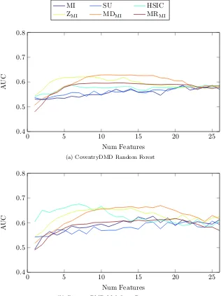
4.14 Classification AUC scores for the CoventryDMD with the MI,

SU, HSIC,ZM I,M DM I andM RM I selection methods . . . 91

4.15 Histogram of the number of times ranks were assigned to the bias

features by the MI, SU, HSIC,ZM I,M DM I, andM RM Iranking

methods for the RCD, CoventryDMD and WarwickDMD . . . . 93

5.1 Scatter plots of MI againstP M DM I . . . 101

5.2 Permutation distributions of features with increasing

dimension-alities computed from a common target . . . 102

5.3 Scatter plots of MI andZM I againstP M DM I . . . 104

5.4 Scatter plots of MI andZM I againstP CM I . . . 105

5.5 Mean AUC scores achieved over ten evaluations when selecting

between one and twenty features from the Musk 1 and TR 11

datasets . . . 109

5.6 Computation times for theM ImRM R,SU mRM R,ZM ImRM R

andP CM I methods to rank all features in simulated datasets . . 114

6.1 Processing methods for data, using PCA, MI and Feature

Ex-traction in different orders . . . 121

6.2 Carriageway classification AUC when selecting features using the

(16)

6.3 Road-type classification AUC when selecting features using the

different selection paths . . . 124

6.4 AUC performances when between one and five features were

se-lected in the first stage from the CoventryDMD, using ZM I,

P mRM R, Symmetrical Uncertainty (SU) andSU mRM R . . . . 129

se-lected in the first stage from the RCD with carriageway labelling,

usingZM I,P mRM R, SU andSU mRM R . . . 130

se-lected in the first stage from the RCD with road labelling, using

ZM I,P mRM R, SU andSU mRM R . . . 131

se-lected in the first stage from the OARD, usingZM I, P mRM R,

SU andSU mRM R. . . 132

6.8 AUC performances for the CoventryDMD and RCD with

car-riageway labelling when features were selected with one feature

per signal in the first stage . . . 133

6.9 AUC performances of the Random Forest classifier for the RCD

with road labelling and the OARD when features were selected

with one feature per signal in the first stage . . . 134

6.10 Redundancies measured in P CM I for different numbers of

fea-tures selected from the CoventryDMD usingSU mRM RandP mRM R

in a two-stage selection process with between one and five features

selected in the first stage . . . 136

fea-tures selected from the RCD with carriageway labelling using

SU mRM R andP mRM R in a two-stage selection process with

(17)

fea-tures selected from the RCD with road labelling usingSU mRM R

andP mRM Rin a two-stage selection process with between one

and five features selected in the first stage . . . 138

fea-tures selected from the OARD usingSU mRM R and P mRM R

in a two-stage selection process with between one and five features

(18)

List of Tables

3.1 List of signals recorded in the RCD. . . 35

3.2 Label counts for the carriageway and road ground truths . . . 36

3.3 Secondary tasks drivers performed in the CoventryDMD . . . 38

3.4 The protocol for the WarwickDMD experiment . . . 40

3.5 Example of theN-back test with a block of 10 numbers . . . 40

3.6 p-values from two wayt-test and ANOVA for the physiological and selected signals of the vehicle telemetry data streams . . . . 46

3.7 Details of datasets from the UCI and Tuned IT repositories . . . 51

3.8 List of statistical and structural features extracted from each sig-nal from the RCD, CoventryDMD, WarwickDMD and OARD . . 53

4.1 List of signals taken from the RCD, the CoventryDMD, and the WarwickDMD . . . 71

4.2 Rank positions by MI, SU, HSIC, ZM I, M DM I and M RM I for illustrative signals of the RCD, the CoventryDMD and the WarwickDMD . . . 84

5.1 Number of times features selected by M ImRM R outperformed those selected by P mRM R, and vice versa, for each classifier over all train-test iterations . . . 110

5.2 Number of times features selected by SU mRM R outperformed those selected by P mRM R, and vice versa, for each classifier over all train-test iterations . . . 110

(19)

5.4 Total number of the original features from each dataset ranked

in the top five by M ImRM R, SU mRM R, and P mRM R for

different split types and a deform type of{5,10,20,30,40}% . . . 112

6.1 Redundancy for the eight selection algorithms measured by SU of

top ten features selected from the CoventryDMD, RCD-carriageway,

RCD-road, and OARD datasets . . . 141

6.2 WarwickDMD features ranked byP mRM R in a two-stage

pro-cess with one feature selected per signal in the first stage . . . . 142

6.3 Mean AUC performances when building models for different

com-binations of drivers and testing on individual driver data for the

distraction status (normal ordistracted) and a increase in heart

rate (baseline orincrease by 5 bpm) . . . 145

6.4 AUC performances for each train-test iteration with data from

individual drivers to predict the distraction status (normal or

distracted) and an increase in heart rate (baseline orincrease by

(20)

CHAPTER

1

Introduction

Driving is a safety critical task that requires a high level of attention and

work-load from the driver [123, 124, 125, 168]. Despite this, people often perform

secondary tasks such as eating or using a mobile phone, which increase

work-load levels and divert cognitive and physical attention from the primary task of

driving [140]. As well as these distractions, the driver may also be overloaded

for other reasons, such as with an incident on the road or holding conversations

in the car.

This problem of driver distraction has several potential solutions. The first,

is to remove the driver from the system with autonomous or self driving vehicles.

The technology for self driving cars is still being developed, however, and there

are many social, legal, and ethical issues to overcome before they are adopted

widely [98, 133]. Another approach is to reduce the number of tasks a driver

performs, or by simplifying the driving task [18, 150]. For example, adaptive

cruise control and automatic breaking systems are designed to reduce the

com-plexity of driving [96]. Such driver assistance systems introduce new issues that

also cause inattention, however, either because the driver is under-stimulated

and their attention lapses or because they trust the vehicle to perform tasks

that it is incapable of [19].

Another solution to this distraction problem is monitor the workload levels

of the driver [73, 161, 167], and limit the functionality of in-car devices while the

driver is overloaded [114]. This can take the form of withholding an incoming

phone call or delaying the display of non-urgent vehicle information. It may also

be possible to warn the driver when they are inattentive, or have the vehicle

(21)

1. Introduction

1.1 Driver inattention monitoring

Driver monitoring can be performed in various ways, from monitoring the

ve-hicle’s external environment to directly measuring the driver’s physiology. The

external environment provides insight into the driver’s workload through the

characteristics of the road or type of terrain [131, 132]. The driver’s physiology,

can be used to directly assess the current workload of the driver [57, 99, 127],

but physiological sensors are more intrusive. Video processing methods can also

be applied to analyse the posture, head position, and gaze of the driver, but

cameras systems can be expensive and unreliable in poor light conditions or

when the driver wears glasses. A third approach, and one that is taken in this

thesis, is to use the driving behaviour and vehicle telemetry to assess workload

of a driver.

1.2 Vehicle telemetry data

Telemetry data typically consists of measurements over time, often at high

sam-ple rates. This thesis is concerned mainly with the analysis of vehicle telemetry

data, although its contributions are relevant to temporal data found in other

do-mains, including medicine, environmental monitoring and activity monitoring.

In general the measurements are made by sensors in a system or environment [3].

Electrocardiogram (ECG) sensors in the medical domain, for example, record

measurements of current across a patient’s chest, and for earthquake detection

a seismometer measures movements in the ground.

Sensors in vehicles communicate via a Controller Area Network (CAN)-bus

[29, 30, 69], which is a broadcast protocol on which all nodes receive any

mes-sage sent over the network. Node identifiers are sent within mesmes-sages and nodes

are able to ignore messages that are irrelevant to them to avoid becoming

over-loaded. In a modern vehicle there are over 50 sensors providing over 1000

telemetric signals, including those that measure wheel speeds, Steering Wheel

(22)

1. Introduction

other aspects. All these sensors communicate over the CAN-bus, and because

a broadcast protocol is used it is possible for a data logger to connect to and

record all messages they send.

1.3 Data mining

Data mining is the process whereby data is turned into patterns to describe a

part of its structure [3, 61, 71, 84, 160]. Data is in abundance and is generated

in almost all fields, from science to business and from media to transport. This

is largely due to the ease and inexpensiveness of storing data, allowing decisions

to be deferred to subsequent processing that may not yet be developed. There

are several difficulties in processing such data, including the computational

re-sources required and avoiding useless, uninteresting or spurious findings.

In the automotive industry data is produced in and analysed by a range

of business divisions, including research and development, manufacturing, and

after-market care [78]. In this thesis, the data mining of vehicle telemetry data

is considered. Vehicle telemetry data is recorded in higher detail and for more

tasks than ever before, including fault detection and diagnosis (e.g. [20, 43, 72,

175]), road type, surface and pot-hole detection (e.g. [25, 60, 83, 103, 144]),

and driver monitoring for both safety and comfort concerns (e.g. [114, 130, 151,

152, 161]). We develop techniques that aim to minimise spurious findings from

vehicle telemetry data in these tasks, while still ensuring that those findings

are interesting and useful. Furthermore, to allow the data mining process to

be performed within a reasonable time, we address the issue of computational

expense in the proposed techniques.

1.4 Problem statement and contributions

This thesis aims to apply data mining techniques to vehicle telemetry data

(23)

prob-1. Introduction

lem statement is: Can a data mining methodology be developed that

enables non-intrusive estimation of the current workload levels of a

driver using telemetry data? To have estimation of the current workload

levels, models must take inputs from vehicle telemetry from only a short period

prior to the current time where the estimation is being performed. The models

must also be reliable enough to allow the vehicle to confidently adapt to the

workload level of the driver, by either reducing its functionality or intervening

in dangerous situations. In developing a data mining methodology for

process-ing telemetry to produce such models for estimatprocess-ing driver workload, this thesis

makes the following main contributions:

1. Developing an unbiased relevancy measure for temporal

vari-ables based on the permutation method.

Selecting features from large feature sets is an example of the Multiple

Comparison Procedure (MCP), which is responsible for input selection

er-rors, over-fitting, and over-searching [65]. Permutation methods have been

proposed as a solution to the MCP and are used to assign significance to a

test statistic, with respect to the null hypothesis of the observation being

insignificant. Permutation methods cannot be directly applied to

tem-poral data, however, and there are several approaches to using them in

ranking features. To apply permutation methods to temporal data,

there-fore, we use a blocking strategy in a similar manner to Kirch [75] and

Adolf et al. [2], and introduce a new strategy of using random block sizes.

Furthermore, to rank features we propose two non-parametric methods of

normalising a correlation statistic that can be used in a feature ranking.

2. Establishing a method for feasibly computing unbiased feature

redundancies using the permutation method.

The naive approach for computing redundancies using the permutation

method is extremely expensive computationally. Each individual

(24)

be-1. Introduction

tween them. Typically, P is in the order of thousands, which means

Mutual Information (MI) is computed thousands of times for each

per-mutation method between two variables. For relevancy computations of

mfeatures, this number of correlation computations is multiplied toP m.

When redundancies between variables are considered, the computational

complexity increases toO(P m+P m2), which is infeasible for many feature

sets. We therefore propose a method for estimating the unbiased

correla-tions by comparing permutation correlacorrela-tions computed during relevancy

comparisons. This method is then used in feature selection frameworks

such as minimal Redundancy Maximal Relevance (mRMR) [113].

3. Using known redundancy structure in features extracted from

signal data with signal selection, feature extraction, and feature

selection.

The selection of model inputs is an important stage of the data mining

process, as too many or bad inputs can cause issues in both model

perfor-mance and complexity. As well as selecting from features extracted over

sliding windows of telemetric signals, selection can also take place directly

on the raw telemetry. Selecting from raw signals, although more

compu-tationally efficient, may harm performance of models built on the data.

Extracted features can also be selected on a per-signal basis, considering

the redundancies between features extracted from the same signal first.

The selected features can then be combined for a second stage of selection

to produce the final feature set. This possibly allows for redundancy

be-tween the features to be better removed, and should improve performance

of models that use them.

4. Advancing the process of feature selection from vehicle telemetry

data for classification problems such as driver workload

estima-tion.

(25)

1. Introduction

models for classification tasks, such as classifying the current road-type

and estimating workload levels of the driver. In particular this

method-ology will focus on selecting features to use as inputs to such predictive

models that determine parameters of the driving environment and driver.

The models will then be evaluated to estimate their performance and

de-termine the efficacy of the proposed methodology.

A final contribution, supplementary to developing a data mining

method-ology, is the production of publicly available datasets for driver monitoring

research. The Road Classification Dataset (RCD) is collected over several

jour-neys and is presented as an environment classification problem. The ground

truth is the current road type the vehicle is on, and the workload level of the

driver can be estimated from this [128, 132, 136, 172]. Town roads, for instance,

entail different levels of workload than highways [131]. To estimate the current

workload level more directly, the ground truth of the Warwick-JLR Driver

Mon-itoring Dataset (WarwickDMD) is taken from physiological sensors.

Physiolog-ical measures, including Heart Rate (HR) and Electrodermal Response (EDR),

recorded from such sensors have been shown to change with respect to workload

in past research (e.g. [13, 99, 126, 136, 167]). This means that they can be used

to estimate the current workload of the driver and be converted to labels in

training data for predictive models to estimate workload. A final ground truth

is taken from the activity of the driver at a particular moment in time, which

includes normal driving and driving with secondary tasks.

1.5 Structure of thesis

The remainder of this thesis is structured as follows:

Chapter 2provides the necessary background for this thesis. The proposed

data mining methodology, based on the general data mining process [3, 70, 160],

is presented. The general data mining process describes how data should be

(26)

pre-1. Introduction

dictions. With some specialisations, the methodology described can be applied

in building predictive models from vehicle telemetry data in the automotive

domain. Two applications of data mining of vehicle telemetry are then

sum-marised, namely environment and driver monitoring.

Chapter 3 describes the datasets that are used throughout this thesis.

Three vehicle telemetry datasets, namely RCD, Coventry-JLR Driver

Monitor-ing Dataset (CoventryDMD) and WarwickDMD are described in detail. The

RCD and WarwickDMD datasets have been made publicly available to aid

research in data mining, and driver and environment monitoring. Further,

statistical analysis of WarwickDMD is presented to confirm findings made by

Mehler et al. [99], Reimer et al. [127]. Finally, other datasets collected in

non-automotive domains and that are available via UCI1 _{and Tuned IT}2

reposi-tories are described briefly. The majority of these datasets are non-temporal

and are used in Chapter 5, where temporal issues regarding the permutation

method are not considered for simplicity. The vehicle telemetry datasets and

the OPPORTUNITY Activity Recognition Dataset (OARD) are used for

ex-periments in Chapter 6.

Chapter 4investigates the application of permutation methods for feature

selection in temporal domains. Permutation methods can be used to normalise

for several biases found in the feature selection process, namely input selection

errors, over-fitting, and over-searching. They cannot typically be applied to

temporal data, however, as one assumption they require is that samples in data

are exchangeable, which is not the case in data with high autocorrelation. This

chapter aims to overcome this limitation through treating the data in blocks,

and it is successfully used in normalising for biases in feature selection using MI.

Five potential ranking statistics are suggested and applied in selecting features

from the three vehicle telemetry datasets.

Chapter 5approaches the issue of redundancy analysis with mitigated

bi-ases using the permutation method. The permutation method itself is expensive

(27)

1. Introduction

computationally and consists of thousands of individual permutations and MI

correlation calculations. The permutation method must be performedm2_times

to compute redundancies betweenmfeatures, which is infeasible in general. To

avoid this computational requirement, a new redundancy measure is proposed

based on the comparison of permutation distributions generated from a

com-mon target variable. This approach requires only mpermutation methods and

efficiently provides allm2redundancies between features. Using simulated data

with features of various noise and bias levels, we show that the approach provides

good estimates of permutation normalised MI. We then apply it in the mRMR

framework to successfully select features from the non-temporal datasets listed

in Table 3.7, having added extra features to increase the bias and redundancy

of their features.

Chapter 6combines the temporal permutation method introduced in

Chap-ter 4 with the redundancy computation approach proposed in ChapChap-ter 5 to

produce a method for selecting features from temporal data using

permuta-tion normalised correlapermuta-tion estimates and considering redundancy. Selecting

signals prior to feature extraction is also considered as this may provide further

efficiency gains in the feature selection process. Finally, a two-stage feature

se-lection process is proposed to take advantage of known redundancy structures

in features extracted from signal data. Here, features are selected first from

individual signals before being combined with those from different signals for a

second selection stage. This two-stage feature selection process is then applied

to selecting features from all of the temporal datasets described in Chapter 3.

Chapter 7concludes this thesis by summarising the research contributions

(28)

CHAPTER

2

Background

The terms data mining, data science, pattern recognition, and machine learning

are used variably in the literature and are often confused with each other, but all

have the common aim of learning patterns and building models from data. This

process of modelling data, or using it to make predictions, has become pervasive

in the modern world and is used across all scientific disciplines. Temporal, time

series or telemetry data mining has been successfully applied in medicine to

monitor patients in real time and for weather and environmental prediction

to predict the weather in the near future or the climate in years to come [3,

160]. Vehicle telemetry from aeroplanes [93], NASA’s space program [163], and

automobiles [20, 60, 78, 102, 103], has been mined for various applications,

including safety improvement, fault detection, or efficiency gains [3].

Data is gathered at unprecedented rates and is often at least partially

un-structured or undefined, which means analysing it is a complex and sometimes

difficult task even for domain experts. The advent of connected sensor

technolo-gies [3] has amplified this as it allows collection of data streams with relative

ease and often at high sample rates. In this chapter the necessary background

of this thesis is covered. In Sections 2.1 and 2.2, the data mining process and

methodology that is used throughout this thesis is outlined. The data mining

methodology is split into the learning approach, which is discussed in Section 2.1,

and evaluation and refinement, which is discussed in Section 2.2.1. Applications

of data mining methodologies in the automotive industry for driver and

(29)

2. Background

Problem deﬁnition

Data collection

Data cleaning

Feature extraction

Sampling

Discretization

Feature selection

Algorithm engineering

Evaluation Data

Engineering Database

Creation

[image:29.595.196.385.135.336.2]

Reﬁnement

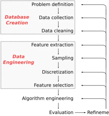
Figure 2.1: Diagram showing the data mining process.

2.1 Data mining process: The learning approach

The methodology used in this thesis is based on the general data mining process

described by John [70], and is outlined in Figure 2.1. Each stage in this process

is linked and it should be iterated on as new findings are made. For instance,

discoveries during data cleaning and exploration will influence decisions in later

stages. As well as this, results from model evaluation will affect decisions in

previous stages, as the learning approach is iterated upon and refined. In this

section the learning approach is discussed, which consists of the Database

Cre-ation, Data Engineering, and Algorithm Engineering components. Each stage

in these components are described in the following sections.

2.1.1 Problem definition

The problem definition should communicate to the investigator what is required

from the data mining process and how to know if it is successful [70]. A problem

can often be formed as a question, for example “what kind of road is the vehicle

(30)

2. Background

roads that exist, and so evaluating any predictions is impossible. An improved

problem statement may then be “is the vehicle currently travelling on a single

or multiple lane road?”. Here, the aim of deciding the road type between a

deterministic set of options is clear to the practitioner.

Even if a problem statement can be understood by the practitioner, however,

it may not be complete. Analysis of the data may discover something new and

unexpected about the domain, which may mean the problem definition requires

some refinement. For example, a third kind of road with no lanes may be

discovered, leading the domain expert and practitioner to expand the current

definitions of the road types or add a third one. If the current definitions

are altered, the problem statement may then read as, “is the vehicle currently

travelling on a road with multiple lanes or not?”.

Finally, any restrictions on the resources or inputs should be clearly defined

[70]. A model that requires the vehicle to travel on the same road for a full hour

before outputting a decision would not be suitable in the real world where most

journeys are shorter than this. A final refinement is therefore needed, where

the problem statement becomes, “is the vehicle currently travelling on a road

with multiple lanes or not? The model should use inputs from vehicle telemetry

recorded in the previous 2.5 seconds only.”.

2.1.2 Data collection

The data collection stage is where a database describing the defined problem is

created [70]. The variables present in the database should describe the

prob-lem appropriately, and the conditions under which they are recorded should be

controlled carefully. For example, a problem statement such as “determine the

stopping distance of the vehicle with differing load weights and an arbitrary

driver on dry and good quality tarmac”, would require a model with inputs

such as the current travelling speed, accelerations and pedal positions. As well

as recording these signals the domain expert may suggest also to record

(31)

2. Background

distribution and allow the model to capture its effects on stopping distance.

Data should be collected using several drivers on dry tarmac roads and with

different load weight distributions, to create a database that fully describes the

problem definition. Collection under conditions other than these will introduce

noise into the database and be detrimental to the performance of models built

on the data [50]. Of course, this is often unachievable due to limits on resources

and difficulties in properly defining the problem.

Collection of vehicle telemetry data is made possible by connecting a data

logger to the Controller Area Network (CAN)-bus [29, 30, 69], which is able

to record all communications between the vehicles control units, such as the

engine, transmission or steering control units. The CAN-bus is a protocol and

medium for sensors and actuators in the vehicle to communicate with one

an-other. Devices are easily connected to a CAN, and receive all data sent over it

but process only messages relevant to themselves. The engine control unit will

receive messages sent by the audio system, for example, but will not process

them. When two devices communicate at the same time, the lower priority

device is able to recognise this and end its communication without affecting or

delaying the higher priority message. Once the higher priority broadcast has

ended, the lower priority device will reattempt its communication.

CAN is an asynchronous event based message protocol where devices

broad-cast messages on events, which can be time based [69]. For example,

Indica-torStatus may be communicated only when it is relevant and the indicator is

being used, and others such asVehicleSpeedmay be broadcast regularly at 5Hz.

These inconsistencies mean that it difficult is to process the data log and build

models on it directly, and so it is typical to re-sample the data at a common

rate, e.g. between 10−100Hz, to produce signals with samples of the same

frequency.

Finally, if the problem is to be posed as one of classification, the ground

truth used to derive the labels or targets must be assigned in a consistent and

(32)

2. Background

lead to noise in the learning process leading to poorer classification results or

invalid conclusions during evaluation. The target variable should be assigned

at the same rate as the signals, with a label for each sample in the data [3, 50].

Often, the database will be made up of several smaller datasets, either

be-cause it was split into drive cycles or bebe-cause it was collected over several

jour-neys. It is often advantageous to maintain the separate datasets and have a

mechanism for combining them throughout the data mining process. This

ap-proach provides greater flexibility than if the datasets were considered as one.

This enables individual journeys to be considered in learning, in order to

cus-tomise models for certain circumstances, and allows training and testing data

to be from separate drive cycles.

2.1.3 Data cleaning and exploration

Once a database is created, it should be inspected to ensure that all variables

were recorded as expected [70, 110]. This is to say, for example, that a signal

named VehicleSpeed represents the speed of the vehicle at the current point in

time. Traditionally, this has been performed by a human analyst, inspecting

each variable for any defects or unexpected characteristics. For instance, value

changes from one sample to the next may be expected to be small, or two

variables might be known to have a high correlation from analysis of other

related data. Observations that are at odds with any expectations may have to

be explained, and in some cases rectified, before any conclusions can be drawn

from the data. For example, rapid deceleration and high suspension activity

is unexpected in data collected during a regular commute. If the commuter

reports performing an emergency stop during that journey, however, this offers

a reasonable explanation for the spurious data. If this event is then seen to

be outside of the problem scope, a judicious practitioner may choose to then

remove this period from the database and minimise its effects on the data mining

process.

(33)

2. Background

noise, bias, or autocorrelation, that may lead to bogus concepts appearing to

be meaningful, or hiding other genuine concepts [70, 110]. This is of particular

concern in vehicle telemetry data as it inherently has high autocorrelation due

to its temporal nature, and data collection efforts invariably lead to datasets

containing signals with biases. Signals related to the duration of a journey, such

as fuel level, often appear highly related to the target variable, even though they

are unrelated to the problem definition. Other signals that are affected by this,

such as yaw rates, accelerations and engine oil temperatures, may also exhibit

minor biases that are not obvious and are unlikely to be noticed by an analyst.

Performing this manual analysis to find issues with large databases is an

extremely expensive task, and many may go unnoticed by the analyst. Typically,

only a small number of key signals that are well understood are inspected and

if these appear to have no issues, the same is assumed of the remainder. In this

thesis, we assume that noise or bias is likely to remain in the database and so

specialised techniques are developed to mitigate them later in the data mining

process during the feature selection stage (Section 2.1.7).

2.1.4 Temporal feature extraction

In temporal data mining, it is advantageous to include historical information

when performing classification [3, 5, 143, 161]. Without this, the current

sam-ple only contains information about the exact point that sensor measurements

were made. This means that no trend or statistical information contained in

signals can be used in determining the classification. We refer to this process of

incorporating historical information into the current sample astemporal feature

extraction, although in some literature it is referred to as motif extraction [3].

In this thesis the same temporal feature extraction process is applied to data

from individual journeys or drive cycles. After feature extraction, they should

again be maintained as separate datasets. A feature is extracted from a signal,

S, by applying a function,f(·), toS over a sliding window of lengthl. At time

(34)

2. Background

signal for the window,

f(st, st−1, . . . , st−l+1) =f(St,l), (2.1)

where St,l is the signal between times t and t−l+ 1. If t < l, because it is

at the beginning of the recorded signal, t samples are used in extracting the

feature. This is performed for all values of t, ensuring that a signal with n

samples produces a feature that contains n samples also to line up with the

target variable,Y.

Features can be split into two categories, namely structural and statistical.

Structural features describe the trend of the signals, whereas variations, peaks,

and averages are represented by statistical features. Several different features

of both types are extracted from each signal over different temporal windows

to produce a set of features,X={X1, X2, . . . , Xm}. Different window lengths,

combined with different features, allow different types of historical information

to be extracted from the signal. Features extracted over large window lengths

may contain more historical information, but may update slowly to changes in

circumstance and be of little value in a real time predictive model. For instance,

during an emergency stop taking 2 seconds, the mean vehicle speed over a 5

seconds sliding window would be non-zero for 7 seconds after the start of the

incident, even though the circumstances have changed drastically. Conversely,

features extracted over shorter window lengths will update more quickly, but

may have higher variance and be more susceptible to noise as they are computed

from fewer values.

Instead of extracting features, it is also possible to automatically learn

fea-tures, through genetic programming [44, 45, 100, 162] or by using deep learning

techniques such as stacks of restricted Boltzmann machines [48, 120]. Both of

these techniques have been successfully applied in learning features, and

catego-rizing images [120], music [48, 100] or performing other classification tasks from

(35)

2. Background

can be used to learn functions to transform data into a set of features that

are more descriptive of the target variable. Genetic programming produces a

function made of basic operations (and potentially of the form shown in

Equa-tion 2.1), selected for performance over generaEqua-tions of mutaEqua-tion, crossover and

reproduction [44]. In deep learning an abstract representation of the data is

produced by using multiple layers of models such as restricted Boltzmann

ma-chines, in which outputs of one layer are used as inputs to the next layer. The

data is input in the first layer and the outputs of the final layer can be used in

predictive models for classification or regression tasks [48].

2.1.5 Sampling

If the data collected has a large class imbalance, models built on it may

in-correctly bias to the majority class. The Road Classification Dataset (RCD)

described in Section 3.1 has almost six times more samples of single lane roads

than roads with multiple lanes. An apparently successful model that predicts

the road has one lane regardless of the input and would still maintain an

accu-racy of over 80%, although this would have little use in reality. One approach

to dealing with this problem is to re-sample the data, by either removing

ma-jority class samples (under-sampling), or generating copies of the minority class

samples (over-sampling) [55].

A simplistic method for under-sampling is to remove samples from the

ma-jority class at random to reduce their number and balance the class distribution.

This potentially removes information from the data, however, and may cause a

model to under-fit. In over-sampling, minority class samples are replicated at

random to increase their number, but this may lead to over-fitting. More

sophis-ticated methods include One Sided Sampling (OSS) [79] and Synthetic Minority

Oversampling TEchnique (SMOTE) [15]. OSS aims to produce the minimal set

of samples to describe the data, removing from the majority class borderline

samples that are close to the decision boundary, and redundant samples that

(36)

2. Background

along the hyper-planes between samples of the minority class. Although this

avoids over-fitting somewhat, it causes the variance of the data to increase and

over-generalises the minority class [15].

Over-sampling and under-sampling techniques are impractical in multi-class

situations, as the minority and majority classes are both hard to define and

re-sample properly [91]. One approach to mitigating imbalance in mutliclass

datasets is to use cost-sensitive learning [55], where different costs are assigned

to misclassifying a sample as a particular label. Assigning higher costs to

mis-classifying a minority class sample than a majority class sample can force the

model to adjust to the imbalance. Alternatively, Error Correction Output

Cod-ing (ECOC) can be applied, which is an ensemble classifier where the multi-class

classification problem is decomposed into several binary classifications, referred

to as dichotomies, and a model is built for each [8]. Re-sampling techniques can

then be applied in each of the dichotomies to fix both imbalance introduced by

the decomposition and any imbalance in the original dataset [91, 135].

Another consideration here is the sample size itself [70]. If there are too many

samples, it may become infeasible computationally to perform an in-depth

anal-ysis of the data, which can be mitigated through sub-sampling. In non-temporal

data, a stratified random sub-sample is used, retaining the original class

distri-butions. For temporal data, taking every tth_{sample is generally sufficient, and}

is equivalent to lowering the recording frequency. This will have the effect of

also reducing the autocorrelation in the data, which is often beneficial for some

algorithms and evaluation strategies. Sub-sampling reduces the amount of data

a model learns from and leads to worse performance, which means sub-sampling

should not be substantial.

2.1.6 Discretisation

Many feature selection methods and learning algorithms are only able to

han-dle discrete data, and so any continuous features are discretised before further

(37)

2. Background

feature can take into blocks of contiguous values. All values of a feature within

one of these blocks are then given the same discrete value. Choosing the block

ranges however is non-trivial, and there are several methods of doing so,

includ-ing equal range or equal frequency binninclud-ing [160]. Equal range binninclud-ing splits

feature values into fixed discrete levels, while equal frequency binning uses

dis-crete levels that ensure balanced distribution in the new feature. Both of these

methods are unsupervised, however, and do not consider the predictive ability

of the features produced.

In a supervised setting the target can be used to define the discretisation

lev-els, in order to maximise the predictive performance of the discretised features.

The widely used Minimum Description Length (MDL) method, for example,

recursively splits the domain of the variable into multiple discrete levels while

maximizing the information gain at each cut point [31]. Others include the

class-attribute contingency coefficient [153], and class-attribute interdependence

maximisation [80].

2.1.7 Feature selection

Feature sets, including those of vehicle telemetry signals, often contain numerous

irrelevant and redundant features, both of which have a negative effect on the

performance and complexity of models built on data [58, 76]. For example, the

door lock status is unlikely to be useful in many situations and engine speed

is highly redundant to the vehicle speed. Supervised feature selection aims

to overcome this by selecting those features that are highly correlated to the

class labels, yet uncorrelated to each other. There are three approaches to this

in general: embedded methods, wrapper methods, and filter methods [46, 76].

Embedded feature selection processes act as part of the training of a machine

learning algorithm, for example in Decision Trees that select features to split on

to give the highest classification performance. Wrapper methods use learning

algorithms to evaluate feature sets, often performing greedy searches through

(38)

2. Background

embedded methods are often specific to learning algorithms [46] and wrapper

methods are computationally expensive [76], filter methods are often preferred.

Filter methods operate separately from the learning process [76]. Although

the performance of features selected using a filter method are somewhat

depen-dent on the learning algorithm used [39], they rank features by their expected

performance generally [76]. A filter for feature selection can be constructed

by ranking features by their individual relevance to the target and choosing a

number of the highest ranked features. Choosing features from such a ranking

does not considerredundancybetween features, however, and is therefore likely

to select several highly relevant features that each contain similar information

about a target. An improvement to this would be a filter that considers feature

relationships, selecting features with the highest performance when combined.

Such filters include, but are not limited to, minimal Redundancy Maximal

Rele-vance (mRMR) [113], feature clustering [9, 87] and particle swarm optimisation

[16, 86], each of which considers feature relationships as well as their relationship

to the target.

In any filter method for feature selection, the relevance and redundancy of

features must be quantified. In some cases, where only linear relationships are

of interest, it can be quantified by Pearson’s Correlation Coefficient (PCC).

Most domains contain non-linear relationships, which can be quantified using

information based correlation estimates such as Mutual Information (MI) [160],

which is discussed in detail in Section 4.4. To apply these information based

approaches to numeric or continuous data the probability density functions of

the variables must be estimated and integrated, and is non-trivial [81, 141]. One

method for estimating entropy with continuous data is to use a Parzen window,

but this requires the selection of parameters that cannot be determined easily

from the data [58]. Another more simplistic approach that is adopted in this

thesis is to discretise the variables [31, 58].

MI increases with the dimensionality of features, which causes rankings to

(39)

Un-2. Background

certainty (SU) aims to normalise for this bias by dividing the MI value by the

entropy of the features. SU still prefers features with many values in some

conditions, however, so the bias is not fully mitigated. Another approach to

normalising against this bias is to use permutation methods [4, 37], which are

explored in Chapters 4, 5 and 6.

Gretton et al. [42] introduced Hilbert-Schmidt Independence Criterion

(HSIC) to quantify non-linear relationships between variables and Song et al.

[137] offer proofs to show that it is unbiased. HSIC is a kernel based method to

quantify the relationships primarily between continuous variables, and is often

applied using the Radial Basis Function (RBF) kernel [137]. Where the forms of

relationship are known, or if the variable is discrete, other kernels exist [137]. It

is common also for one kernel to be used for features and another to be used for

the target variable in a classification task. Applying the kernels to each feature

individually is expensive computationally, and is often infeasible even with the

Cholesky decomposition [7]. HSIC and the Cholesky decomposition is discussed

in further detail in Section 4.4.

2.1.8 Algorithm engineering

The algorithm engineering stage encompasses the selection of the learning

algo-rithm and its parameters. For most problems there are several suitable learning

algorithms available that can be applied with little or no adaptation [70, 160].

Such common algorithms include Na¨ıve Bayes, Decision Tree, Random Forest,

Support Vector Machine (SVM) and many others [160]. Whereas these do not

model temporal artefacts, and rely on information captured in extracted

fea-tures, others such as Recurrent Neural Networks or Hidden Markov Models are

able to capture historical trends implicitly.

Many learning algorithms also require parameters to be set. For example,

the C4.5 Decision Tree [160] takes parameters that determine how aggressively

the tree should be pruned and Random Forest has parameters to set the details

(40)

2. Background

ensemble. These parameters can be optimised using an exhaustive or greedy

search, to find those that produce the model with highest performance, but this

can lead to over-fitting as it is a multiple comparisons procedure [65]. Strategies

to avoid multiple comparisons procedures or mitigate their effects are discussed

in Chapter 4.

2.2 The data mining approach: Evaluation and

refinement

Decisions made in the steps described in Section 2.1, prior to the evaluation and

refinement stages, form alearning approach that defines methods for processing

and learning from data to produce predictive models. Here, this learning

ap-proach is evaluated with respect to the problem definition, in order to estimate

its expected performance in reality. The evaluation of a learning approach on

a database can be split into two parts, namely the structure of the evaluation

procedure, and computing a metric of performance for the learning approach

[63]. The evaluation structure defines how a learning approach is applied on the

data, and the produced model is then used to make predictions on testing

sam-ples. These predictions are then compared against the ground truth to compute

metrics that describe the performance of the model and learning approach.

2.2.1 Structure of evaluation

In an evaluation, a learning approach must be applied on training data to build

a model that is then used to make predictions for testing samples, which we

refer to as a train-test cycle. A train-test cycle should be performed several

times with different training and testing samples to produce a more robust

performance estimate. There are two approaches to this in general, namely

k-folds cross validation and random subset validation [50, 63, 160]. In k-folds

cross validation the data is split into k sub-samples, of which k−1 are used

(41)

2. Background

as the testing dataset, and each test sample is used in exactly one train-test

cycle. Random subset validation, sometimes referred to as bootstrap validation

[160], repeatsktimes the train-test cycle with different random sub-samples of

the same sizes for the training and testing datasets. Whereas in k-folds cross

validation the size of the training dataset is determined by the number of folds,

in random subset validation it can be chosen independently of the number of

train-test cycles. Again, samples not used in training are used as testing data.

With too few samples in the training data a learning algorithm will be unable

to build a model to capture the underlying concepts in the data, and result

in producing pessimistic performance estimates. If the proportion of training

samples is too high when compared to testing samples, the evaluation may

over-fit to the data and produce optimistic performance estimates.

Ink-folds cross validation, or in each train-test cycle of random subset

vali-dation, the subsets must be randomly sampled [63]. If the data is non-temporal

or has very low autocorrelation, a simple random sub-sample of the data can

be used for training and the remaining samples used for testing, as these will

provide distinct sets of samples. In cases with high class imbalance, a stratified

sampling procedure may be considered to maintain the class distributions in

the training and testing datasets. Vehicle telemetry data has high

autocorrela-tion, however, and the values of many signals such as V ehicleSpeed or target

variables such as road type, change rarely with time. This means that random

sampling results in the training and testing datasets containing effectively the

same samples, even though they are in fact distinct.

Autocorrelation in data is reduced through linear sub-sampling, where every

tthsample is taken [27], but the amount of sub-sampling required is difficult to

determine, and the issues caused by autocorrelation may not be rectified fully.

When evaluating models for temporal data in this thesis, therefore, contiguous

blocks of samples from journeys or drive cycles are sampled. There are two

methods for doing this, which can be used to investigate different hypotheses.

(42)

2. Background

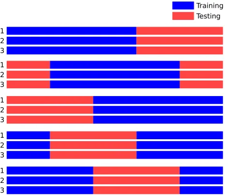
Training Testing

1 2 3

[image:42.595.181.417.282.483.2]

1 2 3

(43)

2. Background

training data, and samples from the remainder used as testing data, which

is similar to the subject-level training adopted by Zhang et al. [173]. This

investigates whether a model can be built using data collected on one journey

and used on future journeys, which may be data collected with different drivers

or vehicles. Second, a contiguous block of samples can be taken from the same

position proportionally in each journey or drive cycle and combined to make

the training data for each train-test cycle, as pictured in Figure 2.2. Here, the

remaining samples from each drive cycle are then used as testing data. This

approach is similar to the segment-level training used by Zhang et al. [172],

but with only one contiguous training block. In each of the k iterations, the

beginning of the training data is at_ki, whereiis the iteration index starting with

0 to ensure an even spread over the train-test iterations. In the first iteration

the beginning of the training data is at time 0 in each drive cycle. For example,

the training data for the second iteration of 20 begins after ₂₀1 = 5% of the

journey length, and the 20thbegins at 19₂₀ = 95%. Although individual blocks of

samples have a high linear autocorrelation, the correlation between them will be

low to produce training and testing samples that do not have the same values.

Regardless of how the data is sampled, any analysis in the learning approach

must be performed on the training data only [50, 63, 160]. This includes the

computation of discretisation levels, selection of model inputs, and optimisation

of model parameters. Any information taken from the testing data may cause

optimistic performance estimates. Furthermore, although the performances on

testing datasets can be used to select the best learning approach, the

perfor-mance estimate produced will be optimistic as the testing data is used in its

selection. To avoid this, and create an unbiased performance estimate for the

best learning approach, a third validation dataset should be used. A validation

dataset can be generated by removing samples from the training data and acts

as a testing dataset in train-validation cycles. Train-validation cycles can again

be performed several times to increase the confidence in performance estimates

Data mining of vehicle telemetry data

University of Warwick institutional repository:

http://go.warwick.ac.uk/wrap

A Thesis Submitted for the Degree of PhD at the University of Warwick

http://go.warwick.ac.uk/wrap/77645

This thesis is made available online and is protected by original copyright.

Please scroll down to view the document itself.

Data Mining of Vehicle Telemetry Data

Phillip Taylor

Doctor of Philosophy

Department of Computer Science

Abstract

Acknowledgements

Declarations

Abbreviations

Contents

List of Figures

List of Tables

CHAPTER

1

Introduction

1.1

Driver inattention monitoring

1.2

Vehicle telemetry data

1.3

Data mining

1.4

Problem statement and contributions

1.5

Structure of thesis

CHAPTER

2

Background

2.1

Data mining process: The learning approach

2.1.1

Problem definition

2.1.2

Data collection

2.1.3

Data cleaning and exploration

2.1.4

Temporal feature extraction

2.1.5

Sampling

2.1.6

Discretisation

2.1.7

Feature selection

2.1.8

Algorithm engineering

2.2

The data mining approach: Evaluation and

refinement

2.2.1

Structure of evaluation