Copula methods in econometrics

(1)

University of Warwick institutional repository: http://go.warwick.ac.uk/wrap

A Thesis Submitted for the Degree of PhD at the University of Warwick

http://go.warwick.ac.uk/wrap/60167

This thesis is made available online and is protected by original copyright. Please scroll down to view the document itself.

(2)

University of Warwick

Doctoral Thesis

Copula Methods in Econometrics

Author:

Kazim Azam

Supervisor:

Dr. Gianna Boero

Prof. Michael Clements

A thesis submitted in fulfilment of the requirements

for the Doctorate of Philosophy

in the

(3)

List of figures

vi

List of tables

viii

Acknowledgments ix

1 Introduction 1

2 Dependence Analysis between Foreign Exchange Rates: A Semi-Parametric

Copula Approach 6

2.1 Introduction . . . 6

2.2 Semi-Parametric Copula Framework . . . 10

2.2.1 Copula Families . . . 10

2.2.1.1 Gaussian Copula . . . 10

2.2.1.2 SJC Copula . . . 11

2.2.2 Time-Varying dependence . . . 12

2.2.3 Marginal Specification . . . 15

2.2.4 Estimation . . . 16

2.3 Short-comings (Dynamic Copula) . . . 17

2.3.1 Simulation . . . 18

2.4 Data . . . 20

(4)

Contents iii

2.5 Copula Results & Economic Interpretation . . . 21

2.5.1 Pre-Euro . . . 21

2.5.2 Post-Euro . . . 23

2.5.3 Recent-Crisis . . . 25

2.6 Conclusion . . . 28

3 Marginal Specifications and a Gaussian Copula Estimation 38 3.1 Introduction . . . 38

3.2 Gaussian Copula Setup . . . 41

3.2.1 Parametric Copula Specification . . . 42

3.2.2 Semi-Parametric Copula Specification . . . 43

3.2.2.1 Empirical Distribution Fej . . . 44

3.2.2.2 Unknown Fj . . . 44

3.3 Bayesian Estimation . . . 45

3.3.1 First Stage p(β, z|Θ) . . . 46

3.3.1.1 Parametric Margins . . . 46

3.3.1.2 Unspecified Marginals . . . 47

3.3.2 Second Stage . . . 48

3.4 Data Generating Process . . . 48

3.5 Marginal Specifications . . . 49

3.6 Simulation . . . 50

3.6.1 Setup . . . 50

3.6.2 Bias & Variance . . . 51

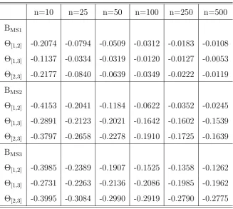
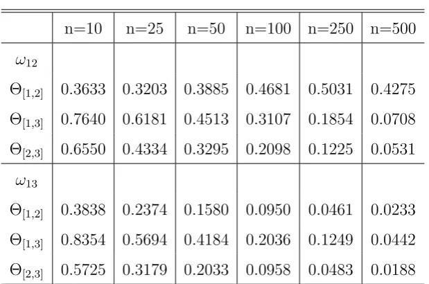
3.7 Results . . . 52

3.7.1 Bias . . . 52

3.7.2 MSE . . . 53

3.7.3 Non-Copula Alternative . . . 56

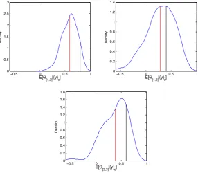
3.7.4 MS1 Kernel Density . . . 57

(5)

Contents iv

4 Bayesian Inference for a Semi-Parametric Copula-based Markov Chain 63

4.1 Introduction . . . 63

4.2 Copula-based Time Series (Review) . . . 66

4.2.1 Copula-based Markov chain . . . 66

4.2.2 Copula Mixing Properties . . . 69

4.2.3 Copula Estimation . . . 71

4.2.3.1 Full Parametric Approach . . . 71

4.2.3.2 Semi-Parametric Approach . . . 72

4.2.4 Non-Parametric Approach . . . 73

4.2.5 Discrete Marginals . . . 73

4.3 Framework . . . 76

4.4 Bayesian Sampling Scheme . . . 78

4.4.1 Sampling from p(U|Y; Ψ) . . . 79

4.4.2 Sampling from the Posterior p(Ψ|U) . . . 81

4.5 Alternative Models . . . 83

4.6 Data Example (Firearm Homicides) . . . 84

4.7 Further Discussion . . . 87

4.8 Conclusion . . . 88

I

Annexes

90

A Annexes to Chapter 3 91 A.1 Copula Families and Conditional Distribution . . . 91

A.1.1 Copula Transformations . . . 91

A.1.2 Clayton Copula . . . 91

A.1.3 Gumbel Copula . . . 92

A.1.4 Gaussian Copula . . . 92

A.1.5 Student-t Copula . . . 93

A.2 Re-Parametrization . . . 94

(6)

Contents v

(7)

List of Figures

2.1 Perfect dependence distance . . . 14

2.2 Fitted Correlation: GARCH-Copula & DCC . . . 20

2.3 Pre-Euro TV-SJC (τ_tU −τ_tL) tail differences . . . 27

2.4 Post-Euro TV-SJC (τU t −τtL) tail differences . . . 27

2.5 Recent-Crisis TV-SJC (τ_tU −τ_tL) tail differences . . . 27

2.6 Daily DM/USD Exchange Rate . . . 35

2.7 Daily GBP/USD Exchange Rate . . . 35

2.8 Daily JPY/USD Exchange Rate . . . 35

2.9 Pre-Euro TV Gaussian Copula . . . 36

2.10 Post-Euro TV Gaussian Copula . . . 36

2.11 Recent-Crisis TV Gaussian Copula . . . 36

2.12 Pre-Euro TV SJC Copula . . . 36

2.13 Post-Euro TV SJC Copula . . . 37

2.14 Recent-Crisis TV SJC Copula . . . 37

3.1 Posterior Density of E(Θ|y), n= 10. . . 58

(8)

List of Figures vii

4.1 Mapping of generated ut . . . 77

4.2 DAG of Latent Variable . . . 78

4.3 Firearm Homicides South Africa . . . 84

4.4 Trace Plots: Gumbel & Gaussian Copula . . . 86

(9)

List of Tables

2.1 MSE from DCC and GARCH-Copula . . . 19

2.2 Pair-Wise Linear Correlation . . . 21

2.3 Sample Statistics . . . 31

2.4 ARMA(p,q)-GARCH(1,1) . . . 32

2.5 Constant Copula Results for DM-GBP, EURO-JPY and GBP-JPY . . . . 33

2.6 Time-Varying Copula Results . . . 34

3.1 Bias for all Marginal Specifications . . . 53

3.2 MSE ratio . . . 55

3.3 Kendall’s rank correlation (bias and MSE) . . . 56

4.1 Posterior Distribution Inference (Firearm Homicides) . . . 86

(10)

Acknowledgments

I am particularly grateful to Gianna Boero, Michael Clements and Michael Pitt for

their continuous support and guidance, and to Valentina Corradi, Adam Johansen and

Andrew Patton for their invaluable advices. I would also like to express my gratitude to

Federica Liberini, Shereyar Malik, Nicola Pavanini and Craig Thamotheram. Comments

from Michael Smith, Claudia Czado, Aleksey Min and Anastasios Panagiotelis at the

4th Workshop on Vine Copula Distributions and Applications (2011), and Copulae in

Mathematical and Qunatitative Finance (2012) are gratefully acknowledged. I am also

thankful for the valuable feedback from the participants of the the Warwick Lunchtime

Workshop. Responsibility for the remaining errors is solely mine.

(11)

Chapter 1 -Introduction

This thesis consists of topics and issues related to copula modelling in Econometrics.

Copula models provide an alternative to joint distribution analysis, which is frequently

required in Economics and Finance.

Measures of dependence is mostly restricted to linear correlation among some random

variables of interest. Embrechts et al. (2002) points out the limitations for such methods,

as linear correlation is only one of the many measures of stochastic dependence.

Multivari-ate Normal and t-distribution have frequently been used to measure dependence between

assets, Hansen (1994), Harvey and Siddique (1999) and Engle and Manganelli (2004)

employ such models for applications to risk-management and portfolio allocation. Other

models such as Multivariate GARCH by Engle and Kroner (1995) and Dynamic

Condi-tional Correlation (DCC) of Engle (2002) have also been applied, but they present various

estimation problems in higher dimensions, and are also bounded by elliptical distributions

for the multivariate analysis. In case a specific distribution is considered, problems can

arise, however there are other methods to consider for multivariate analysis like

General-ized Method of Moments (GMM) which require no assumptions on the distribution.

Recently Copula models have seen an increase in their use in finance and economics,

though being around since Sklar (1959) theorem. They had success in applications, where

dependence is non-linear and the random variables involved have different marginal

dis-tributions. It provides a framework which is general across different type of data types

(12)

2

(marginal behaviour), unlike other joint non-linear modelling where problems are dealt

with in a case-by-case method. There are various copula families available to capture

com-plex dependence patterns, such as non-elliptical forms and tail dependence. In finance,

Embrechts et al. (1999) show how for a Value at Risk (VaR) analysis, the assumption

of multivariate Normal fails to capture joint observations in the tails, and hence apply

copula methods. Cherubini and Luciano (2001) use them for pricing analysis of various

assets. Embrechts et al. (2003) and Rodriguez (2007) study financial contagion through

copula families. Bouy´e et al. (2007) present a detailed coverage of copula methodology

and other applications in finance. Common to all these works is the emphasis on how

copula models provide a solution when we want to have joint analysis with either

non-normal marginal distributions or mixture of different type of marginals. At the same time

when joint distributions are no more best characterised by elliptical distributions, then

using copula models avoids any possible misspecification of dependence measure through

linear correlation.

In Economics instead, the copula based literature remains limited to few studies.

Em-pirical analysis involving discrete data is unavoidable in economics, and alike using other

joint modelling techniques, copula models represent complications. Munkin and Trivedi

(1999), using discrete micro data show how generally joint modelling is troublesome, and

the problem increases when the marginal distributions belong to different parametric

fam-ilies. Chib and Winkelmann (2001) specify a joint discrete distribution, without explicitly

mentioning using a copula. Smith (2003) uses copula framework to study self-selection

problem. Cameron et al. (2004) analyse a selection model with discrete outcomes in a

copula framework. Demarta and McNeil (2005) among others, analyze categorical data

from clinical trials. Zimmer and Trivedi (2006) employ a trivariate copula for

depen-dency between health insurance status for married couples and their demand for health

care. Trivedi and Zimmer (2006) provide details of their use in health economics

applica-tions. Patton (2006) introduces copulas in modelling of economic time series (continuous

data). Hoff (2007) applies a Multivariate Gaussian copula on survey data of different

(13)

3

We now give a formal definition to a copula function. According to Sklar (1959)

the-orem, any p-dimensional joint distribution H of some random variables Y1, . . . .Yp can be

decomposed to a copulaC measuring their dependence, and their marginal distributions

F1, . . . , Fp, specifying their individual characteristics (fat tails, skewness etc.). Formally

given as

H(y1, . . . , yp) = C(F1(y1), . . . Fp(yp)).

Where C : [0,1]p _7→ _[0_,_{1]. The copula} _C _{is unique, if all the margins} _F

1, . . . , Fp are

continuous. The copula could also be stated as,

C(u1, . . . , up) = pr (U1 ≤u1, . . . , Up ≤up).

uj is the uniform variable computed through the marginal distribution,uj =F(yj), where

j = 1, . . . , p. The process of obtaining the uniforms is known as Probability Integral

Transformation (PIT) (see Diebold et al. (1998)). If the joint distribution F is p-times

differentiable, then by taking its pth _{cross-partial derivatives we get}

f(y1, . . . , yp) =

p Y j=1

fj(yj)·c(F1(y1), . . . , Fp(yp)).

Such a decomposition provides a very flexible framework, where each Fj could belong

to a different parametric family, and the dependence among the random variables is not

confined to elliptical distributions (Gaussian or t-distribution). Nelson (2006) and Joe

(1997) cover various statistical and mathematical properties of copulas, including

estima-tion techniques.

We present the abstracts from the chapters of this thesis in the chronological order

now.

Not only currencies are assets in investor’s portfolio, but also central banks use them

for implementing various economic policies. This can create some form of dependence

among different exchange rates. We investigate the dependence pattern among the time

series of daily Deutsch Mark (DM) (Euro later), Great Britain Pound (GBP) and the

Japanese Yen (JPY) exchange rate, all considered against the U.S. Dollar during various

(14)

4

restrictions of linear correlation, a flexible semi-parametric copula methodology is adopted

where the marginals are non-parametric and the copula is parametric, to capture richer

dependence form. Dependence is estimated as a constant measure and also allowed to vary

over time. Our approach is the first time, where a time-varying copula parameter is

con-sidered in a semi-parametric setting avoiding any possible marginal misspecification, along

with a depth full analysis of the dependence patterns among such vital currencies. During

the Pre-Euro period, we find slightly more dependence when both DM (Euro)/USD and

GBP/USD jointly appreciate as compared to joint depreciation, especially in the late 90s.

Such results are reversed for GBP/USD and JPY/USD in the early 90s. In Post-Euro

period, DM (Euro)/USD and GBP/USD exhibit stronger dependence when they jointly

appreciate, which could indicate preference for price-stability in EU zone. Whereas the

dependence of JPY/USD with both DM (Euro)/USD and GBP/USD is stronger when

they jointly depreciate, this could imply preference for export competitiveness among the

countries. In the beginning of Recent-Crisis period, DM (EURO)/USD and GBP/USD

show stronger dependence when they jointly depreciate, but later during the period, we

see the similar tendency for these exchange rates to be related more when they jointly

appreciate. Such measures of asymmetric dependence among the exchange rates provide

vital insight into Central banks preferences and investors portfolio balancing.

Multivariate analysis involving random variables of different data type like count,

continuous or mixture of both is frequently required in econometrics. A Copula based

methodology can be adopted for such data, where the association among the random

variables is independently modelled from their specific marginal distributions. Depending

upon the chosen marginal specifications, copula estimation proceeds. A semi-parametric

copula estimation, where the marginals are specified empirically performs very well, but

for discrete data its appropriateness is questioned (see Genest et al. (1995)). Hoff (2007)

proposes a methodology where the marginal distributions are left completely unspecified

and the copula parameters are estimated based on the order statistics of the observed data.

We conduct an analysis to determine the effect on the estimates of a Gaussian copula due

(15)

5

the bayesian approaches to copula estimation, to compare the effects of various marginal

specifications on copula estimates, which is our contribution towards the literature on

Markov chain based time series models. Through employing a Bayesian framework, we

find that treating the marginal distributions as unknown outperforms both assuming an

empirical distribution or misspecifying the marginal distributions, in terms of bias and

mean square error for the estimates of the copula parameters. Hoff’s method particularly

outperforms the other specifications, when one or more of the marginals involved is of low

count data type (binary).

Time series modelling can be very restrictive when accounting for various marginal

specifications (non-normal distribution), data types and the dependence structure through

time. On the contrary, Copula models allow such issues to be specified independently of

each other. We propose a general technique to model a univariate strictly stationary time

series through a copula. The novelty lies in the fact that it can be applied to both discrete

and continuous data, and is invariant to any copula family. The technique is robust to

any marginal mis-specification, and we successfully capture persistence in a time series

through a copula. Expanding the methodology of Hoff (2007) for cross-sectional data,

we set out a Bayesian sampling scheme to estimate the copula parameters, based only

on the order statistics of the observed data. To show it’s applicability, a real time

se-ries (weekly firearm homicides in Cape Town, South Africa) is used, and we are able to

successfully capture the persistence in such a series. In terms of the Bayesian

methodol-ogy, the technique performs well (fast mixing and low autocorrelation). Such a method

(16)

Chapter 2 -Dependence Analysis between Foreign Exchange

Rates: A Semi-Parametric Copula Approach

§

2.1 _Introduction

Exchange rates are a vital aspect of International Economics, used to implement

vari-ous economic policies. Along with GDP and interest rate, exchanges rates are an indicator

of a country’s economic outlook, and are determined through various cross-country

eco-nomic fundamentals. In this era of globalisation, countries are not simply interested in

closely monitoring their own currencies, but also the currency of other countries, which

causes them to frequently intervene in the foreign exchange market. Such an intervention

to guide their currency in a particular direction due to another currency, creates a

depen-dence among the exchange rates. A synchronisation of business cycles, or difference in

short-term interest rates across countries causing capital inflow/outflow, can also create

comovement of exchange rates. Currencies are also held in investors portfolio along with

other financial assets, and their preference over holding such currencies, also creates a

relationship between the exchange rates.

Not only are the exchange rates dependent upon each other, they could also exhibit

non-linear dependence and non-constant dependence through time. Takagi (1999) states

if there are two countries, A and B, who export to foreign countries and in order to

(17)

2.1. Introduction 7

sure their export prices are competitive to each other, then if country A’s exchange rate

depreciates, country B would ensure their exchange rate does too, which creates joint

depreciation dependence. On the other hand if the countries prefer price stability among

each other (maybe regional), then if country A’s exchange rate appreciates, country B

will intervene in the foreign exchange rate to ensure similar appreciation of their currency,

and hence causing dependence due to joint appreciation. The variation in the preference

of being competitive in terms of export, or ensuring price stability, creates an

asym-metric dependence among the two currencies. Patton (2006) shows that Deutsch Mark

and Japanese Yen (both against U.S. Dollar) before the introduction of the Euro, tend

to exhibit stronger dependence when they jointly depreciate, as compared to when they

jointly appreciate. Dias and Embrechts (2010) report similar results for the same

curren-cies, but over different periods. Boero et al. (2011) show such asymmetric dependence

patterns vary for different currencies. Another contributing reason for such asymmetric

dependence patterns could be associated to the common denominating currency in the

two exchange rates. U.S. Dollar has long been considered as a reserve currency, meaning

investors prefer to hold it more in their portfolio as compared to the other currencies. So

when U.S. Dollar appreciates, investors forgo their holdings of other currencies and shift

their funds into the U.S. Dollar. On the other hand, when U.S. Dollar depreciates, they

might not prefer to hold other currencies similarly. Such shifting of funds to and from

the U.S. Dollar could also create an asymmetric dependence. These asymmetries are not

only found in exchange rates, but also for other financial assets, Longin and Solnik (2001)

show assets returns exhibit stronger dependence during market downturns as compared

to market upturns. This paper aims to understand such phenomenon among Deutsch

Mark (DM) (later Euro), Great Britain Pound (GBP) and Japanese Yen against the U.S.

Dollar (USD) through different economic periods.

Patton (2006) adopts the copula methodology for time-series analysis and identifies

higher dependence between DM (Euro) and JPY (both against dollar) when they are

both depreciating, as compared to when they are both appreciating. Dias and Embrechts

(18)

2.1. Introduction 8

Both Patton (2006) and Dias and Embrechts (2010) report such results for a constant

and time-varying measure of dependence. Boero et al. (2011) perform similar analysis

over several exchange exchange rates including GBP against the U.S. Dollar, but only for

a constant measure of dependence over time. All these work show that dependence varies

over different periods, for example before and after introduction of Euro. We extend

previous analysis and investigate dependence between exchange rate before and after the

euro, and over the recent financial crisis period.

Copula methodology requires the decomposition of the marginal distributions of the

random variables from the dependence among them. Patton (2006) and Dias and

Em-brechts (2010), adopt a fully parametric approach, where the marginals are chosen from a

parametric family along with a parametric copula. In their case, they assume the exchange

rate returns to be specified throught-distribution, with varying degrees-of-freedom. The

copula estimation relies on no misspecification of the marginals, and hence any parametric

family chosen requires testing for the appropriateness of the chosen marginals

specifica-tion. It is easy to misspecify the marginals, especially when the time-series in question is

of high frequency (daily exchange rates). Genest et al. (1995), show how non-parametric

marginals produce consistent and asymptotically normal copula estimates, given the

un-specified margins are of continuous type. Kim et al. (2007) also show such a specification

to produce efficient results for sample size larger than 100. Boero et al. (2011) adopt

such an approach, which is generally termed as semi-parametric copula estimation. We

extend the approach of Boero et al. (2011) to a time-varying dependence measure within

a semi-parametric copula framework, which is the first time such a flexible approach to

avoid any marginal specification has been considered in a dynamic setting.

We employ two copula families, the Gaussian copula and Symmetrized Joe-Clayton

(SJC) copula of Patton (2006), to measure dependence patterns between DM (EURO)/USD,

GBP/USD and JPY/USD. The time-varying measure of dependence for both copula

evolves according to a ARMA type process, same as Patton (2006). The SJC copula is a

two parameter based copula measuring the lower and upper joint tail dependence

(19)

2.1. Introduction 9

returns through a ARMA(p,q)-GARCH(1,1) model to obtain i.i.d observations required

for the copula methodology, and then using the filtered returns we estimate both constant

and time-varying measure of dependence between the 6-pairs for before (1990 - 1998) and

after Euro (1999 - 2006), and for the recent crisis (2007 - 2009).

Using the Gaussian copula, we find strong dependence between DM (Euro)/USD and

GBP/USD, especially before the introduction of Euro, which can be associated to how

GBP/USD shadowed the DM (Euro)/USD in the early 90s. The dependence between DM

(Euro)/USD and JPY/USD is much smaller compared to the previous pair, and similarly

for GBP/USD and JPY/USD. The SJC copula however provides a better fit in terms

of likelihood, and reports some asymmetric tail dependence patterns for GBP/USD and

JPY/USD. After the introduction of the Euro, the SJC copula reports higher probability

of joint appreciation between DM (EURO)/USD and GBP/USD, which could be

associ-ated with higher co-operation within the EU for price stability in the region. Both DM

(Euro)/USD and GBP/USD when paired with JPY/USD show similar asymmetric

re-sults, but the time-varying measure reports periods where there is a higher probability to

jointly depreciate as compared to probability of jointly appreciating. In the recent-crisis

period, for DM (Euro)/USD and GBP/USD, the constant SJC copula measure could be

misleading as both tend to jointly depreciate with greater probability, then compared to

joint appreciation in the beginning of 2007, but later revert back to appreciating jointly

with greater probability. This could be associated to the uncertainty the crisis caused

in the beginning of the crisis, and both countries (being in the EU region) adopting

an export competitive behaviour, whereas the dependence between JPY/USD and the

other two exchange rate seems weaker. Generally our results indicate greater preference

for price stability between DM(Euro)/USD and GBP/USD, which is understandable after

the integration of the EU. Whereas, when paired with JPY/USD, more export competitive

behaviour is suggested and investors view JPY/USD as an alternative to DM (Euro)/USD

and GBP/USD, hence the negative correlation reported in time-varying Gaussian copula.

We start our analysis by first explaining the copula methodology in Section 2, where

(20)

2.2. Semi-Parametric Copula Framework 10

non-parametric margins. Section 3 sets out the data, and describes some vital summary

statistics. In Section 4, we present the results for both the constant and time-varying

copula measures and present some economic intuition for the result. Finally concluding

in Section 5.

§

2.2 _{Semi-Parametric Copula Framework}

We presented the copula definition for a multivariate case of dimensionpin Chapter 1.

In our empirical analysis, we are interested in capturing dependence among two random

variables at a time, hence from now we will present the specifications forp= 2 (bivariate).

Instead of denoting the random variables asY1 and Y2, we denote them as X and Y and

their respective PIT asu and v.

2.2.1 Copula Families

There exist a wide array of copulas families to chose from, depending upon the type

of dependence a practitioner is interested in capturing. Nelson (2006) describes most of

the commonly used copulas. Our main aim is to capture any asymmetric dependence

among exchange rates, and show that in the presence of such asymmetries, a Gaussian

copula would provide an inferior fit and fail to capture vital aspects. We will consider only

two copula families for our analysis, the Gaussian copula and the Symmetric Joe-Clayton

(SJC) copula. The latter is a two parameter based copula, one parameter capturing the

joint upper tail dependence and the other parameter the joint lower tail dependence. In

certain instances a one parameter copula like Clayton copula might provide a better fit,

but we are also interested in the dynamics of asymmetric dependence through time, and

see how both tail dependence measure evolve.

2.2.1.1 Gaussian Copula

A Gaussian copula is the most used copula, along with a t-copula from the elliptical

(21)

margins are assumed/chosen to be normally distributed. It is a symmetric and zero tail

dependence copula. For a bivariate case with uniform i.i.d random variables u and v

between [0,1] (obtained through marginal specifications), the Gaussian copula is given as

Cg(u, v|ρ) = Φg(Φ−1(u),Φ−1(v);ρ)

=

Z Φ−1(u)

−∞

Z Φ−1(v)

−∞

1

2π(1−ρ2₎1₂

×

−(s2₋₂_ρst₊_t2₎

2(1−ρ2₎

dsdt,

where Φ is the Cumulative Distribution Function (CDF) of a standard normal

distribu-tion, Φg(u, v) is a standard bivariate normal distribution andρ the correlation parameter

defined over [−1,1].

2.2.1.2 SJC Copula

In order to capture asymmetric dependence in the tails, we have to employ a copula

which separately parameterizes the left and the right tail. Joe (1997) proposes a copula

termed as “BB7”, also referred as Joe-Clayton copula. It is a two parameter based copula,

given as

CJ C(u, v;τU,τL) = 1−(1− {[1−(1−u)κ]−γ+ [(1−v)κ]−γ−1}−

1

γ₎κ1,

where,

κ = 1

log₂(2−τU₎,

γ = − 1

log₂(τL₎.

When κ= 1, Joe-Clayton copula reduces to Clayton copula, and when γ → 0 it reduces

to Joe Copula. τU _and _τL _{are the parameters of the Joe-Clayton copula, capturing tail}

dependence.

If the limit

lim

δ→1Pr[U ≤δ|V ≤δ] = limδ→1Pr[V ≤δ|U ≤δ] = limδ→1(1−2δ+C(δ, δ))/(1−δ) =τ

(22)

exists, then the copula exhibits upper tail dependence if τU ∈ (0,1] and no upper tail

dependence if τU = 0. In same manner, if the limit

lim

→0Pr[U ≤|V ≤] = lim→1Pr[V ≤|U ≤] = lim→1C(, )/=τ

L

exists, then the copula exhibits lower tail dependence if τL ∈ (0,1] and no lower tail

dependence if τL = 0.

Patton (2006) points out that Joe-Clayton copula tends to report asymmetric

depen-dence, even if the dependence in both tails is perfectly symmetric. He proposes a slight

modification to the Joe-Clayton copula and terms it as “Symmetric Joe-Clayton” (SJC)

copula. It is computed as

CSJ C(u, v; τU, τL) = 0.5(CJ C(u, v; τU, τL) + (CJ C(1−u,1−v; τU, τL) + u + v −1)).

It treats symmetry as a special case and is consistent in reporting any asymmetry. An

alternative technique would be to estimate an asymmetric measure of Kendall’s tau for

joint movements below zero (downwards) and then separately for joint movements above

zero and compare those estimates with SJC copula, however for the SJC copula we are not

able to derive the Kendall’s tau equivalent of the joint upper and lower tail dependence

parameters. By fact they are two different measures, SJC copula measures the dependence

in the extreme of both tails, and an asymmetric Kendall’s tau measure will simply be

defined with a threshold at zero.

2.2.2 Time-Varying dependence

There is evidence that dependence among financial assets does not stay constant over

time (see Bouy´e et al. (2008) and Longin and Solnik (2001)). Such dynamics have great

implications from portfolio diversification perspective and can identify how two assets

behave jointly in various economic conditions. Given that we are dealing with exchange

rates which tend to be highly volatile, we should account for changes in the

contempora-neous dependence.

(23)

ARMA process, both for the Gaussian and the SJC copula dependence parameters. We

assume the functional form of the copula remains constant over time, but the copula

parameters can evolve with time. As Patton mentions, the problem lies in defining the

“Forcing Variable” for the evolution equation, as there is uncertainty to what causes

the variation in the parameters. First we define the evolution of the upper and lower

tail dependence parameter in the SJC copula. Identifying the terms for the evolution of

such parameters is not easy in case of observation driven models. We adopt the same

specification as Patton (2006) for both tails, given as

τ_tU = ΛωU+βUτtU−1+αU·

1 10

10

X j=1

|ut−j−vt−j|

, (2.2.1)

τ_tL = ΛωL+βLτtL−1 +αL·

1 10

10

X j=1

|ut−j −vt−j|

, (2.2.2)

where Λ(x)≡(1 +e−x)−1 is the logistic transformation, which keepsτU and τL bounded

to (0,1). Both (2.2.1) and (2.2.2) are similar to an ARMA(1,10) process, where both the

upper tail τ_tU and the lower tailτ_tL at period t depend upon their respective 1-period lag

and a forcing variable for the time-varying limit probability, which is the mean absolute

difference between ut and vt over the last 10 observations. Different specifications were

also tried, but yielded no major improvements, so we adopted the dynamics specified as

of Patton (2006).

The mean value in both (2.2.1) and (2.2.2) is inversely related to the concordance

ordering of the copulas, value of zero corresponds to perfect positive dependence, 1/3

corresponds to independence and 1/2 implies perfect negative dependence. The choice of

the forcing variable makes a good case, as under perfect positive dependence allutand vt

would be on the main diagonal of the copula support, and under independence scattered

through out the support. For So the average distance from the point to the main diagonal

is acts like an approximation for how close the last ten values of u and v (in time) were

to being perfectly dependent, as difference of zero would imply perfect dependence andα

will have a negative sign. This is indeed a dependence measure, which equates to the value

(24)

[image:24.595.217.418.164.356.2]

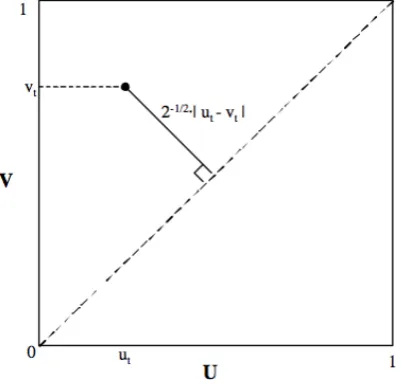
Figure 2.1. Another point to note is the forcing terms in both equations are bound by

the range of value admissible by the LHS variable, as its the absolute difference between

two uniform [0,1] values, hence the average difference will also be bounded between [0,1].

Figure 2.1: Perfect dependence distance

As we saw earlier the Gaussian copula only has one dependence parameter ρ, and we

specify its evolution as

ρt= ˜Λ

ωρ+βρ·ρt−1+α·

1 10

10

X j=1

Φ−1(ut−j)·Φ−1(vt−j)

, (2.2.3)

where ˜Λ(x) ≡ (1−e−x_{)(1 +}_e−x₎−1 _{= tanh(}_x/_{2) is the modified logistic transformation}

required to keep ρt in [-1,1] at all instances. The evolution of ρ is similar to the one

of SJC copula parameters, where in (2.2.3) the lag ρt−1 captures any persistency in the

dependence parameter. To be able to compare the SJC copula dynamics with the Gaussian

copula dynamics a similar MA term is included, which is the mean of the product of the

last 10 standard normals obtained through Φ−1(ut−j) and Φ−1(vt−j). Here this forcing

term is equivalent to efficient Van der Waerden normal-scores rank correlation coefficient,

which again equates to the correlation estimate on the LHS of the equation, being a

correlation coefficient it is also bounded in between [0,1] to correspond by the values

allowed by the LHS.

(25)

ahead forecast for the dependence measure, as for 1-step forecast we would have the

observedxandy (returns in our case) and hence the correspondinguandv. This implies

the forcing terms in all the equations can be computed. For the given set-up, we are

unable to compute dynamic forecasts, for which we would require to change the forcing

terms or be able to first forecastxand y(which would give us predictedu andv), maybe

either through a parametric ARMA(p,q) - GARCH(1,1) set-up, or even a multivariate

equation which would account for the covariance matrix.

2.2.3 Marginal Specification

We just stated the specifications related to the copula families to be used in this paper.

Both the Gaussian and the SJC copula are parametrically specified. Before a copula is

estimated, we need to compute u and v. Let n be the total number of observations,

i= 1, . . . , n, andF and Gbe the marginal distribution function forx and y respectively.

Copula modelling relies upon the assumption that the margins have i.i.d observations,

but daily exchange rate returns tend to exhibit serial correlation and high volatility.

Following the previous literature (see Patton (2006), Dias and Embrechts (2010) and

Boero et al. (2011)), we first apply an ARMA(p,q)-GARCH(1,1) with normally distributed

error term, on each exchange rate return series, through which we obtain the filtered

residuals each assumed to be now independent and identically distributed. Such filtration

still preserves the contemporaneous dependence among the returns. The order ofpandq

for the series along with the results are provided in Table 2.4.

After obtaining the filtered returns, we have to decide the functional form ofF andG.

In practice, the true marginal distribution function are not completely known, and ifF and

Gare misspecified, the employed copula will also be misspecified. An assumed parametric

family for each margin requires careful testing for any misspecification. Assuming that

all the margins are continuous, we can adopt the approach of Genest et al. (1995), where

the margins are left unspecified and computed non-parametrically based on the observed

ranks. Boero et al. (2011) adopt the same approach for the filtered returns. So u and v

(26)

u=Fe(x) = _n₊₁1

n X

i=1

1(Xi ≤x),

v =Ge(y) = _n₊₁1

n X

i=1

1(Yi ≤y),

where ₁(.) is an indicator function and we divide the summation by n + 1 to avoid

CDF boundaries. Fe andGe are employed for allx₁, . . . , x_nandy₁, . . . , y_nrespectively. For

complete clarity, the marginal distribution is not purely non-parametric for the returns, as

first a parametric specification of ARMA (p,q)-GARCH (1,1) is applied to obtain filtered

i.i.d returns. Only then from the filtered returns to obtain uniform random variables for

input arguments to the copula a non-parametric (empirical CDF) specification is adopted.

The novelty of our work lies in that it is the first time a non-parametric (apart from the

filtering) approach has been considered to analyse the time-varying dependence.

Now we can proceed with the estimation of the copula parameters.

2.2.4 Estimation

Given we specified the copula parametrically and the margins non-parametrically, a

semi-parametric estimation technique follows. Let Θ denote the parameter vector

associ-ated to a copula C, required to be estimated. The estimation is performed in two steps,

first the pseudo observations u1, . . . , un and v1, . . . , vn are computed through Fe and Ge,

respectively. Then the second step involves maximum likelihood estimation of the pseudo

log-likelihood function

b

Θ = argmax Θ

n X

i=1

log c(Fe(x_i),Ge(y_i); Θ),

where c denotes the copula density function. Genest et al. (1995) states the

semi-parametric estimatorΘ is consistent and asymptotically normal under suitable regularityb

conditions. Kim et al. (2007) show such an estimator to be robust when the margins are

misspecified. Alternatives to the above estimator would be Inference Function for

Mar-gins (IFM) and Maximum Likelihood (ML) in fully parametric setting (see Joe (1997)).

(27)

2.3. Short-comings (Dynamic Copula) 17

tested, for example Patton (2006) provides a goodness-of-fit test for the margins. Our

approach avoids such issues due to the assumed margins, and only relies on the

assump-tion of the random variables being continues. Kim et al. (2007) show the semi-parametric

estimator to be as efficient as ML, when the sample size is larger than 100.

b

Θ is the estimated constant copula parameters. We are also interested in capturing any

possible dynamics in the dependence parameters through an ARMA process, as described

in Section 2.2.3. The parameters for both the Gaussian copula evolution (ωρ, αρ, βρ) and

for the SJC copula evolution (ωU, αU, βU, ωL, αL, βL) are estimated through maximum

likelihood. The estimated constant copula parameters act as the starting values for the

time-varying dependence measure (i.e. ρ_b=ρ1,τb

U ₌_τU

1 ,τb L₌_τL

1 ).

§

2.3 _{Short-comings (Dynamic Copula)}

Choosing and specifying the dynamics of a time-varying parameter are difficult,

irre-spective of it involving a copula model. For equations (2.2.1) - (2.2.3), we had to find an

appropriate forcing term for the dependence parameter over time. Apart from the chosen

forcing variable, we also tried other specifications, like weighting theuandv observations

to how close they are to the extreme values, and using an indicator based on whether

the observations were in the first, second, third or fourth quadrant. Such variations did

not yield any improvements to the one we used. In all the equations (2.2.1) - (2.2.3), the

values permissible by the terms entering the functional form have the same range as the

dependent variable on the LHS, as they are a approximate measure of dependence through

the previous periods. A drawback to our specification, is the less formidable forcing

vari-able, but this is something commonly encountered in observation-driven based time series

models. It is difficult to map out the true exogenous variation for the dependent variable

of interest. Also previously stated, our approach restricts us for conducting dynamic

fore-casts, which is a strongly desired feature in time series literature. An alternative model to

allow for time variation in the correlation is Dynamic Conditional Correlation (DCC) of

(28)

It is in literature commonly estimated over two-steps, where first a GARCH is specified

for each univariate series and then the equation for the correlation is estimated. We

pro-vide now a detailed simulation benchmark comparison of our copula specification against

the DCC. The comparison can only be done with the time-varying Gaussian copula, as

the DCC permits dependence to be measured only up to the level of correlation, so

un-like copula specifications, no time-varying tail dependence or non-elliptical based time

dependence can be estimated.

2.3.1 Simulation

We will generate 5 different time-varying correlation patterns, as given in Engle (2002),

with an addition of a correlation pattern where the extremes of -0.99 and +0.99 are

observed with high frequency.

• ρt = 0.9 (Constant)

• ρt = 0.5 + 0.4cos(2πt/200) (Sine)

• ρt = cos(t/4) (Fast Sine)

• ρt = 0.9−0.5(t >500) (Step)

T is fixed to 1000 (observations), and after each simulated ρt, we generate two

corre-sponding random variables through separate Gaussian GARCH(1,1) processes given by

h1,t = 0.01 + 0.05r21,t−1+ 0.94h1,t−1,

r1,t =

p

h1,t1,t,

h2,t = 0.5 + 0.2r22,t−1+ 0.5h2,t−1,

r2,t =

p

h2,t2,t,

ρt=Et−11,t2,t,

where the first series is highly persistent. Then we estimate the time-varying correlation

through our GARCH-copula (Gaussian) and the DCC model, and compare the Mean

(29)

Table 2.1: MSE from DCC and GARCH-Copula

Correlation Type DCC GARCH-Copula

Constant 0.0023 0.0030

Sine 0.0292 0.0514

Fast Sine 0.0041 0.0067

Step 0.0066 0.0067

we report the MSE from both time-varying specifications. The MSE from DCC based

time-varying correlation better produces the smaller error in all cases, even though in

terms of the size, they are quite similar. The DCC specification follows the true correlation

pattern quite well, whereas the GARCH-copula’s forcing variable is smoothing over the

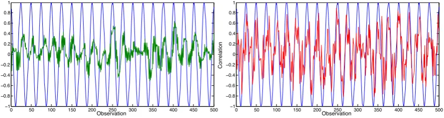
last 10 observations and in doing so misses the rapid correlation changes. We also present

a figure for the Fast Sine based correlation pattern of both the models for one of the Monte

Carlo replication. From Figure 2.2 we see the plotted GARCH-copula fitted dynamics

(green) does not follow the true correlation, whereas the DCC based correlation (red) does

it better. As mentioned this is due to the smoothing of the forcing term, we could reduce

the lags over which we take the expectation in such case. But as we reduce the lags,

the fitted correlation becomes quite unstable. In terms of the modelling approach the

dynamics in such a case are best given by a DCC model. The essence of using a

GARCH-Copula would be to the case for where we might have non-normal joint distribution, where

a non-elliptical distribution best fits the dependence structure. In such cases measures of

dependence beyond correlation have to be adopted. For example, if two random variables

exhibit greater dependence in lower values (lower tail dependence), then measures of

correlation through a multivariate Normal would not appropriately estimate it, as it

assumes no tail dependence (zero correlation within the tails), and we would have to seek

(30)

2.4. Data 20

0 50 100 150 200 250 300 350 400 450 500

−1

−0.8

−0.6

−0.4

−0.2 0 0.2 0.4 0.6 0.8 1

Observation

Correlation

0 50 100 150 200 250 300 350 400 450 500

−1

−0.8

−0.6

−0.4

−0.2 0 0.2 0.4 0.6 0.8 1

Observation

[image:30.595.97.543.95.214.2]

Correlation

Figure 2.2: Fitted Correlation: GARCH-Copula & DCC

§

2.4 _Data

The data consists of daily exchange rates for Deutsch Mark (DM) (later converted at

the conversion rate of Euro), Great British Pound (GBP) and Japanese Yen (JPY). All

these currencies are denoted against the U.S. Dollar (USD). The full sample is over the

period of 1st January 1990 up to 31st December 2009 and collected from Bank of England

database1_{. We converted all the series to obtain log-differenced returns.}

Three sub-samples are considered from the full sample. First, the Pre-Euro period

from 1st January 1990 to 31st December 1998 (2276 observations). Second, the Post-Euro

period from 1st January 1999 to 31st December 2006 (2020 observations) and finally the

Recent-Crisis period from 1st January 2007 to 31st December 2009 (760 observations).

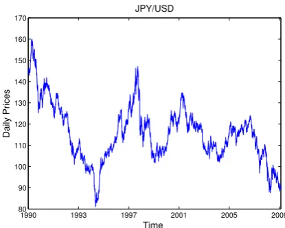
We present time series plots for the three exchange rates in Figure 2.6 - 2.8, and

sum-mary statistics in Table 2.3 for the returns series. Time plots for DM(EURO)/USD and

GBP/USD, show similar trends throughout the sample, especially in the Post-Euro

pe-riod, when both currencies heavily appreciate together. This is also confirmed by the

linear correlation values in Table 2.2, which shows strong correlation in both exchange

rates, even in different sub-samples. JPY/USD on the other hand does not seem to follow

any particular trends with DM(Euro)/USD or GBP/USD, and the correlation seems to

be much weaker, becoming negative with GBP/USD in the Recent-Crisis period.

(31)

2.5. Copula Results & Economic Interpretation 21

Table 2.2: Pair-Wise Linear Correlation

Pre-Euro Pre-Euro Recent-Crisis

EURO GBP JPY EURO GBP JPY EURO GBP JPY

EURO 1 1 1

GBP 0.719 1 0.633 1 0.651 1

JPY 0.500 0.352 1 0.343 0.355 1 0.124 -0.120 1

Table 2.3, shows all of the series have skewness and excess kurtosis. DM/USD in

the Pre-Euro period has almost zero skewness and GBP/USD in the Post-Euro period

has kurtosis of almost 3, but apart from these two cases, none of the other series can

be described through a normal distribution. The Jarque-Bera Statistic rejects normality

with very large values. The ARCH-LM test, suggests the presence of heteroscedasticity for

most of the series, hence it is appropriate for us to employ an ARMA(p,q)-GARCH(1,1)

type filtering for the returns series.

§

2.5 _{Copula Results & Economic Interpretation}

In this Section we present the results from both the constant and time-varying measure

of dependence computed through the Gaussian and the SJC copula. We discuss the

results in detail over the various sub-samples. We seek to answer few questions, first,

whether dependence can be assumed to stay constant not simply across different economic

conditions (over sub-samples), but also within a specific period (within a sub-sample).

Secondly, whether there exist any particular asymmetric dependencies, and the possible

reasons for such patterns.

2.5.1 Pre-Euro

Correlation measures over this period seem to be very high, as compared to the

other sub-samples. The constant Gaussian copula reports correlation of 0.71 between

(32)

linear correlation in Table 2.2. Such strong correlation is not surprising, as the Pound

shadowed closely the Deutsch Mark since 1988 to tackle inflation. The time-varying

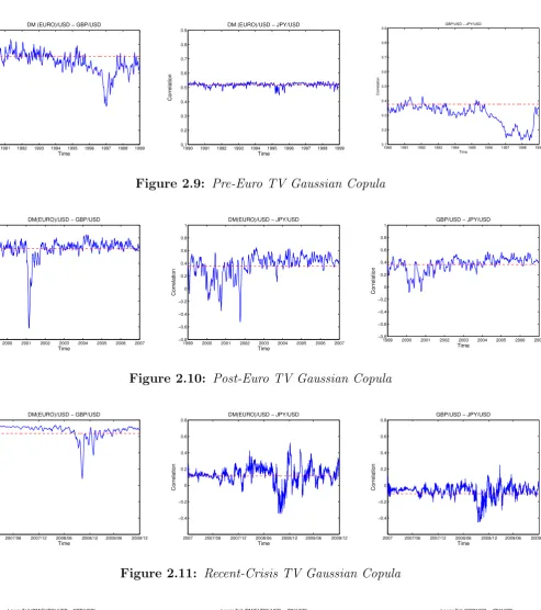
Gaus-sian copula in Figure 2.9 suggests the dependence stayed quite constant among the pair,

except by the end of 1996, where there is a slight decline to about 0.4. Such a decline

could be due to the interest rate lowering announcement in August 1996 by Bank of

Eng-land to tackle inflation. Lower interest rate causes investors to shift their funds from GBP

(causing depreciation), but DM (Euro) did not get necessarily effected by it. The constant

SJC copula results in Table 2.5 suggest no asymmetric dependence, as the differenced tail

dependence measure (τU - τL) is insignificant at 5%. Although the time-varying tailed

differenced series in Figure 2.3 shows after 1993 the difference in upper tail and lower tail

to be negative, this could correspond to greater preference for price stability in the

re-gion. Overall, for dependence between DM(Euro)/USD and GBP/USD, the time-varying

results show that dependence does not stay constant over this period, both for Gaussian

and SJC copula measure.

The relationship between DM(Euro)/USD and JPY/USD seems very stable through

this period. The constant Gaussian copula reports correlation of 0.52 in Table 2.5 and the

time-varying Gaussian shows no deviation from this level in Figure 2.9. Such patterns,

might be suggestive of the fact that these two countries shared similar economic conditions

and had similar foreign trade patterns, which created a unique and constant tie between

them. The constant SJC copula measure reports no asymmetric dependence in Table 2.5,

but from Figure 2.3 we see the difference in the tails of about 0.1. The results indicate

the correlation patterns through a Gaussian copula can be appropriately described by a

constant measure (similar likelihood in Table 2.5 and Table 2.6), the time-varying SJC

copula also does not reveal more information about the dependence through this period,

than what the constant SJC copula reports.

GBP/USD and JPY/USD are among the most volatile currencies, and due to this

volatility investors seek to gain profits from short buying and selling. The correlation is

relatively lower compared to the previous pairs above, of 0.37. The constant Gaussian

(33)

reaches the minimum of 0.1. The constant measure of SJC copula in Table 2.5 suggests

the difference between joint upper and lower tails to be −0.1 and significant at 5%, but

from Figure 2.3, we see the difference in the tails is very volatile and changes sign

fre-quently. To associate such changes due to some form of economic policy of one or both of

the central banks would not be suitable. Investors hold various currencies in their

port-folios and take positions which could imply they shift out (joint depreciation) of the two

currencies in a similar manner. GBP and JPY are not considered as candidates for being

a reserve currency, and investors frequently buy and sell them. Therefore a time-varying

copula should be employed in order to provide a more adequate representation of the

dependence between these pair of currencies.

Unlike Patton (2006), we report the dependence between DM (Euro)/USD and JPY/USD

to be symmetric, but similar to Patton, the time-varying measure of differenced tail

de-pendence is not zero. To remind again we follow a semi-parametric copula estimation,

whereas Patton (2006) sets out a fully parametric copula approach and have a slightly

larger backdating period.

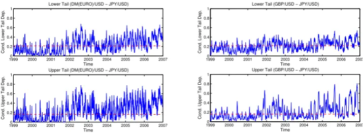
2.5.2 Post-Euro

After the Euro was introduced, now DM (Euro) did not simply represent Germany,

but some major European economies. Not only a single currency was introduced but the

EU was strengthened, where trade policies among all European countries (including Great

Britain) where agreed. The constant Gaussian copula again shows strong correlation of

0.64 between DM (Euro)/USD and GBP/USD, and the time-varying measure in Figure

2.10 suggests also such correlation to have stayed constant, except a dramatic fall in early

2001, which could be due to pessimism about the newly formed currency causing smaller

proportion of DM (Euro) to be held in investors portfolio. The constant SJC copula

mea-sure reports a stronger tendency (τU = 0.36) towards large joint appreciations (τL= 0.53)

with respect to USD, than towards joint depreciation. Such a result could be due to the

strong bounds created by the EU and the preference for price stability through the EU,

(34)

cop-2.5. Copula Results & Economic Interpretation 24

ula in Figure 2.4, we see that at the beginning of the period the difference sometimes in

the tails is reversed, later on the lower tail dependence exceeds that the upper tail. Even

though the constant SJC copula accurately predicts the directions of the asymmetry, it

under predicts the magnitude which at points reaches up to−0.4. This asserts the point

even strongly that among a unified EU pricing stability is more preferred as compared to

having a preference for being competitive in exports. Also Euro is the currency for most

of the European countries, and hence for UK to be competing the rest of the Europe is

very unlikely. The constant SJC copula does report the right sign on the tail difference

in the later half of this period, but the magnitude is surely not appropriate to represent

the period.

The constant Gaussian copula no longer adequately captures the correlation pattern

among the DM(Euro)/USD and JPY/USD. Figure 2.10, shows the correlation goes to

negative values in the infancy of Euro. This again could be due to the uncertainty over

the newly created currency, and investors regarding Yen as a more secure holding in their

portfolios, as compared to Euro. Constant SJC copula measure indicates the tails to be

symmetric, but the time-varying SJC copula in Figure 2.4 shows instances of upper tail

dependence being greater than lower tail dependence, which is understandable as Japan is

not really part of EU trade treaties and now an export competitive position is preferred.

Within this period, for DM (Euro)/USD and JPY/USD, constant measure of dependence

would be misleading and a time-varying copula would be more appropriate.

The correlation between GBP/USD and JPY/USD seems more stable and constant,

also the time-varying Figure 2.10 does not show much deviation from the constant level.

The constant SJC reports no asymmetry, but this is true for the beginning of the period,

but later in the period as we see from Figure 2.4, there is a greater probability of joint

depreciation as compared joint appreciation. The linear correlation for this pair of

curren-cies can be specified through a constant Gaussian copula, but for asymmetric dependence

the constant SJC copula fails to capture the variation in the joint tails.

We cannot compare the results here with previous literature, as our sample for post

(35)

values after the uncertainty due to the new currency.

2.5.3 Recent-Crisis

This period represents turmoil and uncertainty from many aspects. Investor do not

know what currencies to hold. The crisis originated from the U.S. soon had spillover

effects into major currencies. From the constant Gaussian copula results, we see the

correlation between DM (Euro)/USD and GBP was almost the same as in previous

peri-ods. The time-varying measure reveals similar constant correlation until the end of 2008

when correlation dropped significantly, this could be associated to bail-outs of the UK

banks. The SJC constant copula reveals again a significant (at 5%) asymmetry in the

tail, where there is higher probability for these currencies to depreciate together. The

time-varying SJC copula shows in Figure 2.5 that at the beginning of the crisis there is

higher probability to depreciate together. The U.S. Dollar appreciated in the beginning

of the crisis, which is quite unusual given the crisis originated from there. This was due to

short-term interest rate differentials, which investors tried to take advantage of and hence

moved away from Euro and Pound. But such directions were reversed as soon as the risk

aversion abated. Through such times price stability in the EU was strongly among the

agenda, and therefor we see a much stronger probability of joint appreciation between DM

(Euro)/USD and GBP/USD. The time-varying measure for both copulas is more suitable

for this pair of exchange rates in this period.

Between DM (Euro)/USD and JPY/USD, the correlation fell to 0.12. The

time-varying Gaussian copula confirms this in Figure 2.11. By the mid 2008, the correlation

becomes very volatile, which could be due to investors trying to seek safe portfolio

hold-ings. The constant and time-varying SJC copula indicates no asymmetries in the tails.

The correlation between GBP/USD and JPY/USD became negative, −0.12. This is

also confirmed in the time-varying Gaussian copula case, the correlation patterns in late

2008 is similar to the correlation between DM (Euro)/USD and JPY/USD, indicating

sim-ilar positions for Euro and Pound as compared to Yen. The constant and time-varying

(36)

address the extent of negative correlation in late 2008.

In terms of the best copula specification, we see the time-varying SJC copula has the

highest log-likelihood value. As all sub-samples are large, the Akaike Information Criteria

reports the same best fitting copula.

Overall, we discussed few reasons for observing dependence patterns for the currencies

considered, though there could be many more reasons for observing these patterns. We

have not discussed the role of USD, which through out the years has served investors as

a reserve currency and movements to/from USD to other currencies might not be the

same. Exchange rate is not only an economic tool for policy implementation, they are

also considered an asset along with other stock assets. But unlike other financial assets,

investors hold projections over economic conditions which lead them to hold specific

hold-ings on currencies, and this could create complex dependence patterns. We need to use

(37)

1990 1991 1992 1993 1994 1995 1996 1997 1998 1999 −0.5 −0.4 −0.3 −0.2 −0.1 0 0.1 0.2 0.3 0.4 Time

Differenced Tail Dependence

DM(EURO)/USD − GBP/USD

1990 1991 1992 1993 1994 1995 1996 1997 1998 1999 −0.5 −0.4 −0.3 −0.2 −0.1 0 0.1 0.2 0.3 0.4 Time

DM(EURO)/USD − JPY/USD

1990 1991 1992 1993 1994 1995 1996 1997 1998 1999 −0.5 −0.4 −0.3 −0.2 −0.1 0 0.1 0.2 0.3 0.4 Time

[image:37.595.18.566.108.249.2]

GBP/USD − JPY/USD

Figure 2.3: Pre-Euro TV-SJC (τU

t −τtL) tail differences

1999 2000 2001 2002 2003 2004 2005 2006 2007 −0.5 −0.4 −0.3 −0.2 −0.1 0 0.1 0.2 0.3 0.4 0.5 Time

DM(Euro)/USD − GBP/USD

1999 2000 2001 2002 2003 2004 2005 2006 2007 −0.5 −0.4 −0.3 −0.2 −0.1 0 0.1 0.2 0.3 0.4 0.5 Time

[image:37.595.25.572.315.457.2]

GBP/USD − JPY/USD

Figure 2.4: Post-Euro TV-SJC (τU

t −τtL) tail differences

2007 2007/06 2007/12 2008/06 2008/12 2009/06 2009/12 −0.5 −0.4 −0.3 −0.2 −0.1 0 0.1 0.2 0.3 Time

[image:37.595.26.388.514.649.2]

(38)

2.6. Conclusion 28

DM (EURO)/USD and GBP/USD act very similarly and are driven in economic

con-ditions regulated by the EU, this creates strong dependence and the European Bank and

Bank of England to co-operate together towards price stability, and hence we observe

strong dependence when they appreciate together. DM (Euro)/USD and JPY/USD prior

to the Euro, show stable correlation, but after the introduction of the Euro the dependence

is stronger when they jointly depreciate which could indicate a preference to stay

com-petitive in terms of export prices. The relationship between GBP/USD and JPY/USD is

quite volatile, as investors seek profitable holdings on these currencies. After the

intro-duction of the Euro, GBP/USD a follows similar correlation with JPY/USD to that of

DM (Euro)/USD and JPY/USD. We see constant measure of correlation/dependence do

not reveal full information, there are times when correlation changes signs and magnitude,

and hence we should employ the time-varying measures of dependence, as compared to

assuming constant dependence.

§

2.6 _Conclusion

Various currencies are related to each other due to economic interaction among

coun-tries and how they are held in investor’s portfolio. Their relationship in various economic

conditions not only can reveal vital information to policy makers, but can also provide

insight to investors for diversification purposes.

Given non-normality of daily exchange rates and joint non-linear dependence among

exchange rate returns, we adopt a semi-parametric copula approach which overcomes

the short-comings of multivariate Normal and t-distribution. Our approach is similar to

Patton (2006) and Dias and Embrechts (2010), but unlike them we do not assume any

parametric distribution for the marginals. Along with a parametric copula we specify the

marginals to be non-parametric. Such a specification is robust to any misspecification of

the marginals. Genest et al. (1995) show an estimator based on the ranks of the observed

(39)

2.6. Conclusion 29

such a specification is robust to any misspecification of the marginals. Boero et al. (2011)

employ a similar technique, but to estimate constant dependence only. We extended their

approach to study dependence in a time-varying case.

We examine the dependence pattern between DM (Euro)/USD, GBP/USD and JPY/USD

in different economic conditions. From using the Gaussian copula and the SJC copula,

we see varying patterns of dependence in period before introduction of Euro, after and

the most recent financial crisis.

We show linear correlation measures do not reveal dependence completely and to

cap-ture any possible asymmetric tail dependence we should adopt a two parameter copula

like the SJC copula. In the Pre-Euro period DM (Euro)/USD and GBP/USD are highly

correlated and such correlation persists through the other sub-samples. A time-varying

analysis however shows that there are periods when the correlation weakens. From

mea-suring asymmetric tail dependence, we find that the constant SJC copula fails to capture

the variation in the joint tails, as there seems to be some pairs which have a higher

probability to jointly appreciate as compared to probability of joint depreciation during

different sub-samples. For DM (Euro)/USD and JPY/USD, correlation is quite constant

as confirmed by the time-varying measure. There does not seem to be any particular

preference from central banks to create export competitive environment or create price

stability. The relationship between GBP/USD and JPY/USD seems very volatile through

all the samples, and there is asymmetric tail dependence which the constant SJC copula

does not completely capture. After Euro’s introduction, DM (Euro)/USD and GBP/USD

become more dependent when they jointly appreciate, reflecting the preference for price

stability of both central banks, this is understandable as EU has trade policies in place,

which are very co-operative and protect EU countries. Although there are certain

pe-riods (early Recent-Crisis period), where the probability to jointly depreciate is higher

than probability to jointly appreciate, this could be due to shifting of funds into USD

from both currencies. Both DM (Euro)/USD and GBP/USD have a similar stance

to-wards JPY/USD, and hence the correlation between DM (Euro)/USD and JPY/USD and

(40)

2.6. Conclusion 30

We show how dependence evolves over time and assuming a constant dependence

mea-sure fails to capture the variations. The whole analysis is performed in a setting which

ensure no misspecification of the marginal behaviours (distributions). We also prove how

(41)

(42)

(43)

2.6. Conclusion 33 T able 2.5: Constant Copula R esults for DM-GBP, EUR O-JPY and GBP-JPY Pre-Euro P ost-Euro Recen t-Crisis DM-GBP DM-JPY GBP-JPY EUR O-GBP EUR O-JPY GBP-JPY EUR O-GBP EUR O-JPY G BP-JPY Gaussian Copula ( ρ ) 0 . 717 ∗∗∗ 0 . 516 ∗∗∗ 0 . 377 ∗∗∗ 0 . 635 ∗∗∗ 0 . 360 ∗∗∗ 0 . 355 ∗∗∗ 0 . 635 ∗∗∗ 0 . 116 ∗∗∗ − 0 . 103 ∗∗∗ (0 . 007) (0 . 013) (0 . 017) (0 . 011) (0 . 018) (0 . 018) (0 . 017) (0 . 036) (0 . 036) LL − 817 . 0 − 349 . 5 − 172 . 3 − 520 . 4 − 140 . 0 − 142 . 31 − 196 . 5 − 5 . 168 − 4 . 013 SJC ( τ U) 0 . 547 ∗∗∗ 0 . 296 ∗∗∗ 0 . 133 ∗∗∗ 0 . 360 ∗∗∗ 0 . 161 ∗∗∗ 0 . 160 ∗∗∗ 0 . 404 ∗∗∗ − − (0 . 016) (0 . 025) (0 . 030) (0 . 028) (0 . 032) (0 . 031) (0 . 039) ( τ L ) 0 . 554 ∗∗∗ 0 . 315 ∗∗∗ 0 . 231 ∗∗∗ 0 . 530 ∗∗∗ 0 . 215 ∗∗∗ 0 . 218 ∗∗∗ 0 . 526 ∗∗∗ 0 . 064 − (0 . 015) (0 . 025) (0 . 026) (0 . 016) (0 . 029) (0 . 029) (0 . 026) (0 . 045) ( τ U t − τ

L )t

(44)

(45)

2.6. Conclusion 35

1990 1993 1997 2001 2005 2009

1.4 1.6 1.8 2 2.2 2.4 2.6

Time

Daily Prices

[image:45.595.191.398.44.209.2]

DM(EURO)/USD

Figure 2.6: Daily DM/USD Exchange Rate

1990 1993 1997 2001 2005 2009

0.45 0.5 0.55 0.6 0.65 0.7 0.75

Time

Daily Prices

[image:45.595.188.397.285.450.2]

GBP/USD

Figure 2.7: Daily GBP/USD Exchange Rate

1990 1993 1997 2001 2005 2009

80 90 100 110 120 130 140 150 160 170

Time

Daily Prices

JPY/USD

[image:45.595.189.397.524.690.2]

(46)

2.6. Conclusion 36

1990 1991 1992 1993 1994 1995 1996 1997 1998 1999 0.1 0.2 0.3 0.4 0.5 0.6 0.7 0.8 0.9 Time Correlation

DM (EURO)/USD − GBP/USD

1990 1991 1992 1993 1994 1995 1996 1997 1998 1999 0.1 0.2 0.3 0.4 0.5 0.6 0.7 0.8 0.9 Time Correlation

DM (EURO)/USD − JPY/USD

1990 1991 1992 1993 1994 1995 1996 1997 1998 1999

0.1 0.2 0.3 0.4 0.5 0.6 0.7 0.8 0.9 Time Correlation

[image:46.595.60.554.19.576.2]

GBP/USD − JPY/USD

Figure 2.9: Pre-Euro TV Gaussian Copula

1999 2000 2001 2002 2003 2004 2005 2006 2007 −0.8 −0.6 −0.4 −0.2 0 0.2 0.4 0.6 0.8 1 Time Correlation

GBP/USD − JPY/USD

Figure 2.10: Post-Euro TV Gaussian Copula

2007 2007/06 2007/12 2008/06 2008/12 2009/06 2009/12 −0.4 −0.2 0 0.2 0.4 0.6 0.8 Time Correlation

GBP/USD − JPY/USD

Figure 2.11: Recent-Crisis TV Gaussian Copula

19900 1991 1992 1993 1994 1995 1996 1997 1998 1999

0.2 0.4 0.6 0.8 1 Time

Cond. Lower Tail Dep.

Lower Tail (DM(EURO)/USD − GBP/USD)

19900 1991 1992 1993 1994 1995 1996 1997 1998 1999

0.2 0.4 0.6 0.8 1 Time

Cond. Upper Tail Dep.

Upper Tail (DM(EURO)/USD − GBP/USD)

19900 1991 1992 1993 1994 1995 1996 1997 1998 1999

0.2 0.4 0.6 0.8 1 Time

Lower Tail (DM(EURO)/USD − JPY/USD)

19900 1991 1992 1993 1994 1995 1996 1997 1998 1999

0.2 0.4 0.6 0.8 1 Time

Upper Tail (DM(EURO)/USD − JPY/USD)

19900 1991 1992 1993 1994 1995 1996 1997 1998 1999

0.2 0.4 0.6 0.8 1 Time

Lower Tail (GBP/USD − JPY/USD)

19900 1991 1992 1993 1994 1995 1996 1997 1998 1999

0.2 0.4 0.6 0.8 1 Time

Upper Tail (GBP/USD − JPY/USD)

[image:46.595.364.551.39.159.2]