ECE-420: Discrete-Time Control Systems Project Part B: Feedback Control

1

ECE-420: Discrete-Time Control Systems

Project Part B: Feedback Control

In this part of the project you will first simulate an open loop discrete-time system in both Matlab and Simulink, and then modify both the Matlab file and the Simulink file for a simple closed loop system. You will need to modify the project files from the last project assignment for this. You should also look at the last project for more information on how the embedded system toolbox works, it will not be repeated here or in future projects!

Mathematical Background and Review:

Consider a simple discrete-time transfer function with input R z( ) and output Y z( ),

1 2

0 1 2

1 2

1 2

( ) ( )

( ) (

( ) )

1

b b z b z

Y z B z

R z a

G

z a z A z

z

− −

− −

+ +

= =

=

+ +

Cross multiplying we get

1 2 1 2

1 ( ) 2 0 1 2

( )z z Y z z Y z( ) b R z( ) b z R z( ) b z ( )z Y +a − +a − = + − + − R

In the time-domain this becomes

1 2 0 1 2

( ) ( 1) ( 2) ( ) ( 1) ( 2)

y n = −a y n− −a y n− +b r n +b r n− +b r n−

In Matlab, theAandBarrays are then

[

]

[

]

1 2

0 1 2

1

A a a

B b b b

= =

In Matlab, there will be an equal number of elements in both arrays and they are row arrays (because of the way we constructed them). Let’s assume that N denotes the maximum number of coefficients in the transfer function.

For the plant we denoted the arrays as Ap and Bp, with Nbp elements. For a controller, which you will implement in this lab, we will denote the arrays as Ac and Bc, with Nbc elemenets.

2 1) Modify the file openloop_DE.slx to generate both a Matlab and a Simulink simulation of the unit step response for a sampled version of the continuous time transfer function

2

100 ( )

2 200 p

s s

s s

G = +

+ +

We want a sampling interval Ts = 0.01 seconds, and the final time to be Tf = 3.0 seconds. To convert from the continuous-time to discrete-time transfer function using a zero order hold, use the following Matlab code:

Gp = tf([1 100],[1 2 200]); % continuous-time transfer function

Gp = c2d(Gp,Ts,'zoh'); % discrete-time equivalent

The Matlab file will set up the parameters for the Simulink file, then run the Simulink file, and then plot the results. If you run the file openloop_driver.m you should get a plot like that in Figure 1

Figure 1. Open loop response of the system.

2) We are now going to modify the Matlab model to implement a feedback control system. We will assume we are using the integral controller

1

0.02 0.02 ( )

1 1 c

z z

z z

G = = ₋

− −

and that there is a one sample delayH z( )=z−1in the feedback loop between the input and output.

a) Save openloop_driver.m as closedloop_driver.m, and make all of your changes to closedloop_driver.m

b) Comment out the sim command so we are not running the Simulink.

c) Enter the transfer function for the controller, and be sure to determine Ac (the A coefficients for the controller), Bc (the B coefficients for the controller), and Nbc (the number of B coefficients in the

0 0.5 1 1.5 2 2.5 3

0 0.1 0.2 0.3 0.4 0.5 0.6 0.7 0.8 0.9 1

Time

y

v

al

ue

3 controller). Be sure to enter the sample interval Ts in the tf command so Matlab will understand it is discrete-time transfer function.

d) Enter the transfer function for the feedback element 1

( )

H z =z− . Be sure to enter the sample interval Ts in the tf command so Matlab will understand it is discrete-time transfer function.

e) To get the closedloop transfer function, use the feedback command as follows:

Go = feedback(Gc*Gp,H);

f) Modify the lsim command to use Go to get the closedloop response.

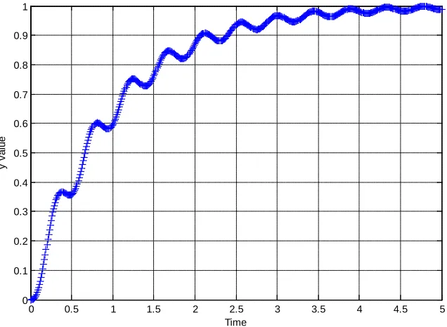
g) If you run the simulation for 5 seconds (and only plot the Matlab results), you should get the plot shown in Figure 2.

Figure 2. Results of the Matlab simulation for the integral controller.

3) Now we are going to modify the Simulink model.

a) Save openloop_DE.slx as closedloop_DE.slx and make all of your changes to closed_loop.slx.

b) Modify closedloop_driver.m to simulate closedloop_DE.slx(modify the argument to sim)

0 0.5 1 1.5 2 2.5 3 3.5 4 4.5 5

0 0.1 0.2 0.3 0.4 0.5 0.6 0.7 0.8 0.9 1

Time

y

v

al

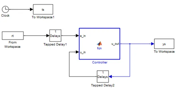
4 c) We are going to first implement the controller by cheating as much as we can. When we are done with this step we want closedloop_DE.mdl to look like Figure 3. You should note two things about this figure, compared with openloop_DE.mdl:

• The inputs (e_in, u_in) and output (u_out) are different

• The order of the input ports are different

• The Plant is now labeled the Controller

You now need to start editing this model. If you do everything correctly, the rest of this project will be easy. It is probably a good idea to open both openloop_DE and closed_loop_DE, find the

corresponding variables (e.g., yout corresponds to uout), and use this a a guide to the correct variable sizes.

i) Change the name of the block to Controller is the easiest, just click on the Plant name and edit it.

ii) Change the input and output variables by clicking on the Controller block and then Simulink and Edit Data icon (see Project Part A). You need to change the variable names, the ports, and make all of the variables functions of Bc, Ac, and Nbc.

iii) You need to edit the code so it uses the variables Bc, Ac, Nbc, e_in, u_in, and u_out. iv) You need to also edit all of the delays in this model to be functions of Nbc.

Figure 3. Initial configuration of closedloop_DE.mdl used for debugging.

d) Now we will test what we have so far. Modify openloop_driver.m. Somewhere before the sim command, rename new variables as follows:

Bc = Bp;

Ac = Ap;

Nbc = Nbp;

5 e) Copy the file closedloop_DE.slx to the file closedloop_DE2.slx (so we don’t screw up what is

already working) and modify closedloop_driver.m to run this new file. Open both closedloop_DE2.slx and openloop_DEslx. Select the plant model (the input, output, and feedback elements) from

openloop_DEand copy them to closedloop_DE2. After some editing, your final system should look like that shown in Figure 4. Note that the input to the plant is now u_in. To make this change, you will need to edit the Plant block and code.

Figure 4. Finals version of closedloop_DE.mdl.

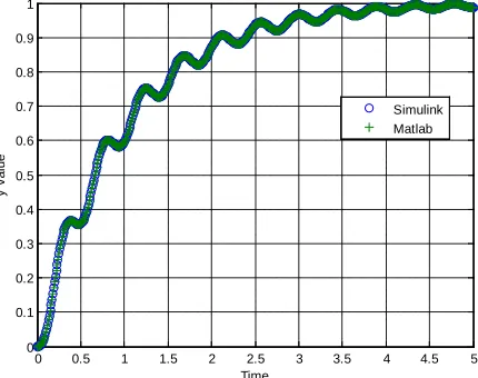
f) Now edit closedloop_driver so you can plot the results from both the Matlab and Simulink results. If you run closedloop_driver you should get the results shown in Figure 5. If you do not get this result, you have done something wrong!

Figure 5. Final results for implementing the feedback control system with the integral controller.

4) Modify you system to use the discrete-time PID controller

2

26.3( 1.74 0.777)

( )

( 1)

c

z z z

z z

G = − +

−

Your simulation results should look like those in Figure 6 (note the final time has been changed). Include this figure in your memo.

0 0.5 1 1.5 2 2.5 3 3.5 4 4.5 5

0 0.1 0.2 0.3 0.4 0.5 0.6 0.7 0.8 0.9 1

Time

y

v

al

ue

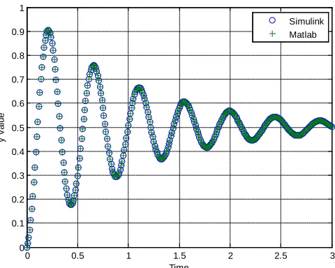
6 5) Modify your simulation to use the proportional+derivative controller, G z_c( ) 12.8(z 0.65 )3

z

−

= . Your

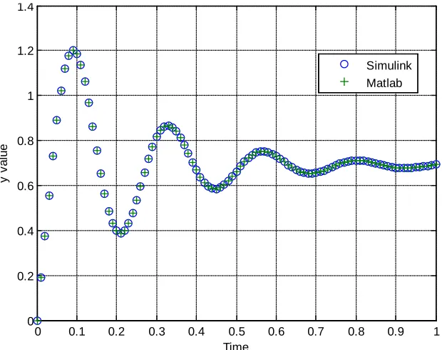
results should look like those in Figure 7. Include this figure in your memo.

To turn in: write a short memo including your graphs (with captions and figure numbers), and any suggestions you may have for improving this part of the project. e-mail me your memo.

Figure 6. Matlab and Simulink results for PID controller.

Figure 7. Matlab and Simulink results for PD controller.

0 0.1 0.2 0.3 0.4 0.5 0.6 0.7 0.8 0.9 1

0 0.5 1 1.5

Time

y

v

al

ue

Simulink Matlab

0 0.1 0.2 0.3 0.4 0.5 0.6 0.7 0.8 0.9 1

0 0.2 0.4 0.6 0.8 1 1.2 1.4

Time

y

v

al

ue