Study and Application of Horizontal Well Productivity Formula with Continuous Time Varying Considered

ISSN Print: 2327-588X

DOI: 10.4236/jpee.2018.69005 Sep. 18, 2018 32 Journal of Power and Energy Engineering

Study and Application of Horizontal Well

Productivity Formula with Continuous

Time-Varying Considered

Chao Liu

, Junting Zhang, Haojun Wu, Bo Zhang, Long Wang

Bohai Oilfield Research Institute of CNOOC Ltd., Tianjin Branch, Tianjin, China

Abstract

The horizontal well technology has been widely applied to enhanced oil re-covery for low permeability and heavy oil reservoir. It is the important basis for designing and optimizing horizontal well to determine the productivity. The productivity determination of horizontal wells in offshore oil fields is mainly based on the actual productivity data of producing directional wells in the similar reservoirs nearby. Considering pressure drop and oil layer thick-ness to calculate the productivity, this method lacks certain theoretical basis and requires rich working experience for reservoir engineers. The other me-thod is Joshi Formula which needs the known horizontal well control radius to be known. But the control radius is man-made at certain degree. In order to address the shortcomings of existing methods, a new reservoir engineering method was proposed to determine the horizontal well productivity formula, horizontal flow pattern and control radius based on the principle of equiva-lent flow resistance and conformal transformation. This method has over-come the disadvantage of determining on person. It provided some theoreti-cal basis for getting the horizontal well productivity and is of some guiding meaning for evaluating the productivity of adjustment wells and development wells.

Keywords

Horizontal Well, Principle of Equivalent Flow Resistance, Conformal Transformation, Control Radius, Pseudo-Steady State Time

1. Introduction

Horizontal well productivity formula has been studied and widely applied from 1940s [1]. It has been numerously researched by domestic and foreign scholars

How to cite this paper: Liu, C., Zhang, J.T., Wu, H.J., Zhang, B. and Wang, L. (2018) Study and Application of Horizontal Well Productivity Formula with Conti-nuous Time-Varying Considered. Journal of Power and Energy Engineering, 6, 32-39. https://doi.org/10.4236/jpee.2018.69005

Received: August 12, 2018 Accepted: September 15, 2018 Published: September 18, 2018

Copyright © 2018 by authors and Scientific Research Publishing Inc. This work is licensed under the Creative Commons Attribution International License (CC BY 4.0).

http://creativecommons.org/licenses/by/4.0/

DOI: 10.4236/jpee.2018.69005 33 Journal of Power and Energy Engineering flow, after which the final productivity formula could be solving by principle of equivalent flow resistance. Babu [6] derived the horizontal well productivity formula through physical model. The domestic researcher Chen Yuanqian [7] got the other horizontal well productivity formula based on Joshi Formula. In the view of mathematical model, Chen Xiaofan [8] simplified the formula initial boundary condition and derived the analytical formula. According to Econo-mides horizontal well productivity formula, Gao Jian [9] analyzed the main in-fluencing factors. Gao Hongmei [10] researched the development of different well productivity formula. Zhang Feng [11] compared and analyzed differences of the horizontal well productivity formula at steady state time between Chen Formula and Joshi Formula. Ding Yiping [12] determined the productivity for-mula of fractured horizontal well multiple transverse cracks by the conception of equivalent radius and analyzed the geometric and physical parameters of reser-voir model and fracture. Xu Guomin [13] studied remaining oil potential tap-ping in the maturing area combined with fine preliminary geological study and horizontal well development technology advantages.

Previous studies have done similar to horizontal wells productivity formula. In the classical formula engineers usually using, there are patterns such as con-trol radius that determines empirically. The productivity formula was improved mainly aimed at this question in this paper. Considering the travel time to the pseudo-steady state time and controlling radius after oil well producing, a new reservoir engineering method was proposed to determine the horizontal well productivity formula based on the principle of equivalent flow resistance, con-formal transformation. It gets accuracy of the formula with the producing well data verifying and has the formula applied in the offshore reservoir adjusting wells proration production. It provides theoretical basis for determining the ho-rizontal well productivity in offshore reservoir and has some directive signific-ance.

2. Methodology

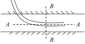
Providing that at the mid of the horizontal homogeneous circular reservoir with constant thickness, there was a horizontal well producing, which showed as Fig-ure 1. The formation and well parameters were known which including that the formation radius is re, the well radius is rw, the horizontal interval is L, the energy

at edge of the formation is too enough to keep the pressure Pe all the time, the

bottom hole flowing pressure is Pwf, the thickness of oil layer is h, the

DOI: 10.4236/jpee.2018.69005 34 Journal of Power and Energy Engineering

Figure 1. The figure of horizontal well

production.

The flow of horizontal well in the horizontal plane can be imaged as that countless vertical wells with length of differential units which radius is dL is producing in the horizontal interval L. As the time increasing, the flow of every well unit could be in pseudo-steady state. At that moment the formula of pseu-do-steady state starting time was introduced:

The start time of pseudo-steady state:

2 t e

s 0.0872 C r

t

K

φµ

= _(1-1)

During the pressure transmission, spread radius is investigation radius ri:

s i

t

3.386 Kt

r

C

φµ

= (1-2)

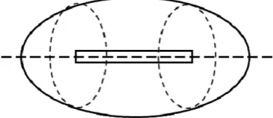
According to the spread radius formula during pseudo-steady state, it could be known that the spread distance of the root and finger on horizontal interval was the longest. The pressure was spread gradually from horizontal interval to exterior of the layer. The flow characteristics of horizontal well were showed as Figure 2.

From Figure 2, it can be seen that the flow of the fluid in the horizontal plane could be approximately recognized as elliptical flow which was showed as Figure 3.

So that the flow of horizontal well can be equivalent to elliptical flow along the horizontal wellbore and plane radial flow along the vertical wellbore. The hori-zontal well productivity could be calculated with the principle of equivalent flow resistance. Providing the elliptical flow resistance in the horizontal plane is Rh

and radial flow resistance in the vertical plane is Rv, the productivity formula is

that:

i wf h

h v

P P Q

R R

− =

+ (1-3) The horizontal plane and vertical plane flow rate formulas of horizontal well were derived.

2.1. Horizontal Well Planar Flow Analysis

According to Zhukovsky conversion, the plan elliptical flow of horizontal well can be converted to circular flow, the formula is:

, ei

z x iy u iv r θ

ξ

ξ

DOI: 10.4236/jpee.2018.69005 35 Journal of Power and Energy Engineering

Figure 2. The figure of flow in the horizontal well production.

Figure 3. The figure of ellipse flow in horizontal

well production.

1 1

2 2

Z

L ξ ξ

 

= _ + _

  (1-5)

1 _{1 cos}

2 2

x _r

L ξ r

ξ

θ

 

= _ + _

 

1 _{1 sin}

2 2

y _r

L ξ r

ξ

θ

 

= _ + _

  (1-6)

2 2

rξ = u +v

2 2

cos u

u v

θ= +

2 2

sin v

u v

θ=

+ (1-7)

According to conformal transformation 1 1

2 2

Z

L ξ ξ

 

= _ + _

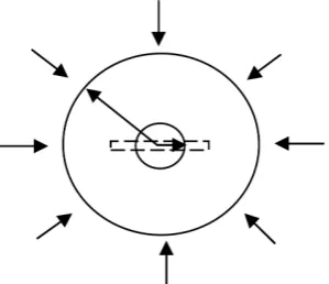
 , the ellipse (long axis is a, short axis is b) is converted to the circle (the radius is (a + b)/0.5L), the area from (−L/2, 0) to (L/2, 0) is mapped into the unit circle, showed as Figure 4.

Providing that there was a vertical well circular flow with radius 1 in circular area with radius (a + b)/0.5L of ξ plane. Considering the thickness of oil layer h

and elliptical radius _b=_a2₋

(

)

  , the flow rate in the horizontal plane

can be calculated with:

(

)

(

)

i wf

hh ₂

2

o

2π

2 ln

2

Kh P P q

a a L

B

L

µ

− =

 _{+ −} 

 

 

 

DOI: 10.4236/jpee.2018.69005 36 Journal of Power and Energy Engineering

Figure 4. The Figure of ellipse flow

con-formal transformation in horizontal well production.

In the formula (1-8) the long axis (a) of the ellipse was considered to equal the spreading radius (ri) plus the half of horizontal interval (L/2) when the well was

producing. So that the expression of value (a) in the formula (1-8) is:

s i

t

2 3.386 Kt 2

a r L L

C

φµ

= + = +

2.2. Horizontal Well Vertical Flow Rate Analysis

According to the conformal transformation, the vertical flow of horizontal well was converted into circular flow. _{ξ = −}1 e−πhZ_1 e₊ −πhZ_

  

  . The strip area in Z

plane can be converted into the circular area in ξ plane. rw in the Z plane is just

as ξw in the ξ plane.

( ) w w w 0,0 2π d d r r Z h ξ

ξ = = (1-9)

When the directional well which flow radius is ξw in ξ plane and horizontal

interval is L, the vertical plan flow rate formula is:

(

)

hv o w 2π ln 2π KL P P q h B r µ − =       (1-10)

The flow resistance formula can be derived by formulas (1-8) and (1-10):

(

)

2 o

h

2 ln

2π 2

a a L

B R

Kh L

µ _ + − _

= _{ }     (1-11) o v w ln

2π 2π

B h

R

KL r

µ

= _(1-12)

The horizontal well productivity formula is:

DOI: 10.4236/jpee.2018.69005 37 Journal of Power and Energy Engineering Including the value a,

(

)

(

)

i wf 2

2

s s

t t

o

w

2π

3.386 2 2 3.386 2

ln ln

2 2π

Kh P P Q

Kt _{L L} Kt _L

C C _{h h}

B S

L L r

φµ φµ

µ

− =

 _{ } 

 _{+ +  +  −} 

 

 _{ } 

 + + 

 

 

 

 

(1-14) The horizontal well productivity formula is show as (1-14). The productivity formula is calculated with horizontal interval, oil layer properties, which solved the disadvantages that the existing formulas could not calculate well controlling radius and controlling area must be given.

3. Application

According to the horizontal well productivity formula, the production of one horizontal well in Bohai A oilfield. And the formula calculation and actual pro-duction data were compared to verify the accuracy of the formula. It was known that according to the horizontal well productivity formula derived in this paper and the properties data of three wells, the theoretical curve of production changed with time. It had good results for the fitting which verified the accuracy of the formula.

The horizontal well technology has been widely applied in offshore reservoir development. It is the important index for producing to calculate the horizontal well productivity. The horizontal well productivity formula has been used to calculate the productivity of four adjusting wells. These wells have been drilled and put on production in Feb. 2014. The results showed that the errors between practical and the theoretical data were very small and the method has some practicality. The results were showed as Figure 5 and Figure 6. The error analy-sis was showed as Table 1 and Table 2.

In the view of Table 1 and Table 2, the production of some adjusting wells was designed with the horizontal well productivity formula. The actual produc-tion data showed that the errors were little enough to confirm the formula relia-ble, which provided the theoretical basis and be applied in determining the pro-duction in offshore oil field.

4. Conclusions

DOI: 10.4236/jpee.2018.69005 38 Journal of Power and Energy Engineering

Figure 5. The production calculation curve of the two horizontal wells in B

oilfield.

Figure 6. The production calculation curve of the two horizontal wells in C

oilfield.

Table 1. The comparison table of actual production data and formula calculation data

in B oilfield.

Oilfield Well name Actual production _(m3_/d) Calculate production _(m3_/d) Error (%)

B oilfield B1H 38.6 35.4 8.23

B oilfield B2M 43.9 39.5 9.96

Table 2. The comparison table of actual production data and formula calculation data

in C oilfield.

Oilfield Well name Actual production _(m3_/d) Calculate production _(m3_/d) Error (%)

C oilfield A4H 145 148.4 2.36

C oilfield A5H 165 159.7 3.21

0 20 40 60 80 100 120

0 100 200 300 400 500 600 700

O

il p

ro

du

ctio

n

（

m

3/d

）

Viscosity（mPa•s）

Theoretical curve Actual data

60 80 100 120 140 160 180 200

0 100 200 300 400 500 600 700

O

il p

ro

du

ctio

n

（

m

3/d

）

Horizontal well length（m）

DOI: 10.4236/jpee.2018.69005 39 Journal of Power and Energy Engineering 3) The production of four adjusting wells in Bohai B oil field was designed with the horizontal well productivity formula. The actual production data showed that the errors were little enough to be applied in determining the pro-duction in offshore oil field.

Conflicts of Interest

The authors declare no conflicts of interest regarding the publication of this pa-per.

References

[1] Li, X.L., Zhao, Z.Y., Liu, M.T. and Zhang, L.P. (2008) An Overview of Horizontal Well Water Injection Technology. Special Oil & Gas Reservoirs, 15, 1-5.

[2] Liu, X., Zhang, X.G., Chen, H., An, F. and Sun, L.J. (2005) A Research Overview of Horizontal Well Water Injection and Oil Production Technology. Journal of Jiang-han Petroleum Institute, 27, 802-804.

[3] Hao, M.Q., Li, S.T., Yang, Z.M. and Liu, X.G. (2006) An Overview of Multi-Lateral Well Technology. Special Oil & Gas Reservoirs, 13, 4-7

[4] Giger, F.M. (1989) Analytic Two-Dimensional Models of Water Cresting before Breakthrough for Horizontal Wells. SPE 15378, 409-416.

[5] Joshi, S.D. (1988) Augmentation of Well Productivity with Slant and Horizontal Wells. SPE 15375, 729-743.

[6] Babu, D.K. and Odeh, A.S. (1989) Productivity of a Horizontal Well. SPE 18298, 417-455.

[7] Chen, Y.Q. (2008) Derivation and Correlation of Production Rate Formula for Ho-rizontal Well. Xinjiang Petroleum Geology, 29, 68-71.

[8] Chen, X.F., Le, P., Su, G.F. and Yang, J. (2010) A New Formula to Calculate the De-liverability of Horizontal Well. Journal of Southwest Petroleum University (Science & Technology Edition), 32, 93-95.

[9] Gao, J., Yue, L., Duan, Y.Z. and Yan, Y.Z. (2003) The Main Factors of Affecting Ho-rizontal Well Production Capacity. Foreign Oilfield Engineering, 19, 16-17. [10] Gao, H.H., Wang, X.M. and Wang, Z.W. (2005) Review of Horizontal Well

Produc-tivity Formulae Study. Xinjiang Petroleum Geology, 26, 723-726.

[11] Zhang, F., Zhao, P.Q., Chen, Y.Q. and Qin, J.M. (2008) Study on Contrast of Two Deliverability Equations of Horizontal Well. Well Testing, 17, 16-18.

[12] Ding, Y.P., Wang, X.D. and Xing, J. (2008) A Method of Productivity Calculation for Fractured Horizontal Well. Special Oil & Gas Reservoirs, 15, 64-68.