Email: [email protected]
Received February 1, 2012; revised March 2, 2012; accepted March 17, 2012
ABSTRACT
Modeling the force-velocity dependence of a muscle-tendon unit has been one of the most interesting objectives in the field of muscle mechanics. The so-called Hill’s equation [1,2] is widely used to describe the force-velocity relationship of muscle fibers. Hill’s equation was based on the laboratory measurements of muscle fibers and its application to the practical measurements in muscle mechanics has been problematic. Therefore, the purpose of this study was to develop a new explicit calculation method to determine the force-velocity relationship, and test its function in experimental measurements. The model was based on the motion analysis of arm movements. Experiments on forearm rotations and whole arm rotations were performed downwards and upwards at maximum velocity. According to the present theory the movement proceeds as follows: start of motion, movement proceeds at constant maximum rotational moment (Hy- pothesis 1), movement proceeds at constant maximum power (Hypothesis 2), and stopping of motion. Theoretically derived equation, in which the motion proceeds at constant maximum power, fitted well the experimentally measured results. The constant maximum rotational moment hypothesis did not seem to fit the measured results and therefore a new equation which would better fit the measured results is needed for this hypothesis.
Keywords: Muscle Mechanics; Muscle Power; Force-Velocity Relationship; Arm Movement
1. Introduction
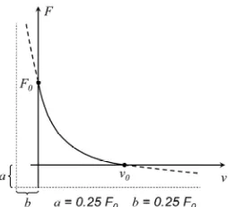
Modeling the force-velocity relationship of muscle-tendon unit involves many different factors. In muscle mecha- nics force-velocity relationship of skeletal muscle is of- ten presented by so-called Hill’s equation (F+a)(v +b) = b(F0 + a), where F is the maximum force within mus-cle contraction, a and b are constants, F0 the isometric force of muscle or the constant maximum force gener-ated by muscle with zero velocity and v is velocity, (Figure 1) [1,2]. This equation was based on the labora-tory measurements in which force (F) of the activated muscle lifted different loads (F = mg) and speed of the load (v) was then measured. In Hill’s equation F is force, a is constants force, v is velocity, b is constant velocity and F0 is constant force. In the equation the vectors of forces and velocities have the same direction and there-fore Hill’s equation can be presented in a scalar form. The left side of Hill’s equation is the product of force and velocity and that is power. As the right side of the equa-tion is constant it can be seen that Hill’s equaequa-tion is a constant power model. Hill’s force-velocity relationship is one of the most essential equations of muscle mechan-ics and it has often been principle object in biomechani-cal studies for about 50 years, e.g. [3-6]. Force measured
from skeletal muscle during maximum tension depends on several internal and external factors. Internal factors are e.g. anatomical structure of muscle (cross sectional area, pennation etc.), fiber type distribution (fast and slow twitch muscle fibers have different force-velocity equations), condition of the muscle (fatigue, training) and muscle length. External factors are e.g. contraction type (isometric, concentric and eccentric) and contraction ve-locity (rate of change of muscle length). Good reviews of the above mentioned factors have been presented, e.g. [4,7,8]. Force (F) creates a moment about the joint which is moment arm multiplied by force (M = r × F). Length of muscle’s moment arm depends on joint angle and it changes as the rotation movement proceeds about the joint axis. The combined effect of the forces of several different muscles produces the rotation movement about the joint axis.
Figure 1. Hill’s equation(F+a)(v + b) = b(F0 + a) where F0 is so-called isometric force or force with zero velocity, v0 is the highest possible velocity, a and b are constant force and constant velocity. In rotational movement torque M corre-sponds to force F and angular velocity φ corresponds to velocity v.
generate within a certain range of velocity. The principle of constant maximum power is the same as in Hill’s equation except that the constant maximum power in the present study is a characteristic of whole muscle group instead of separate muscle fibers as in the Hill’s equation. This study continues the development of the earlier find-ings [11-13].
2. Methods
The experiments in the present study consisted of three different maximum velocity arm movements: 1) forearm rotation downwards, 2) whole arm rotation downwards and 3) upwards. The selection of these movements was based on the earlier findings of Rahikainen and Luhtanen [11] where so called “constant power theory” seemed to work at the last phase of the arm push in shot put. In or- der to study this finding more extensively it was reason-able to choose a simple procedure as represented by arm rotations in the present study. The photographs of arm movements in this study were generated by a special mo- tion camera system [14,15] which represents the move- ment as a series of object images. The paths of the mark lights attached to the moving object can be seen as bro- ken light-lines. The principle of the method is to photo- graph the moving object through a rotating disc which consists of one transparent opening and nine filter open-ings serving as the shutter apertures. As the exposure disc rotates in front of the camera lens (film camera Ca- non T70) and the camera aperture is open, the disc serves as the shutter. This way several overlapping exposures are generated on the same frame. The transparent open- ing generates images of the moving object, and the filter openings generate the light-lines indicating the paths of mark lights attached to the moving object (Figure 2). In this study the speed of rotation of the exposure disc was 300 rotations per minute, exposing five (300/60) object images per second and giving the time interval of 20 ms
Figure 2. Forearm rotation downwards with maximum force. Angle of rotation φ and its corresponding time T (ms) are presented on the subject image.
for nine light-lines between consecutive object images (for more detail, see [14,15]). Figure 2 represents a fore- arm rotation downwards. As seen in the figure the radius of the rotation circle is not exactly the same as the radius of forearm rotation. This is because of a slight motion of the elbow joint. Actually the radius of forearm rotation is slightly larger than the radius of circle on the figure and it can be measured from the forearm image before the start of the rotation movement. Angular velocity mea- surements are calculated with the formula
S R T
(1) in which the length of forearm is the radius of rotation R and the distance measured between two successive measured points on the path of light-lines is the distance increment ΔS.
2.1. Measurement of Rotation Arc
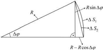
For convenience the arc ΔS1 was measured as a straight
line ΔS2 (Figure 3) and the error between these two va- lues was estimated. The arc ΔS1 can be calculated from the straight line ΔS2 from the formula:
2
1 2
1 arccos 1
2 S
S R
R
[image:2.595.367.478.85.221.2]Formula derivation from the right-angled triangle in Figure 3.
22 2 2 2
2 sin 1 cos
S R R
(2)
2
2 2
2 sin cos 1 2cos
S
R
(3)
2 2
sin cos 1 (4)
2
2 2 2 cos
S
R
rotation, R = length of forearm, arc ΔS1 = distance the mark light travels during the time interval Δt and ΔS2 = the arc
ΔS1 measured as a straight line.
2 2
1
cos 1
2
S R
(6)
2 2 1
1 arccos 1
2
S S R
R
(7)
The maximum value measured from Figure 2 (corre- sponding time 140 ms) is ΔS/R = ΔS2/R = 0.356. Substi-tuting this value in the formula above (7) the arc of rota-tion is obtained as ratio form ΔS1/R = 0.358. It can be seen that ΔS2 fits with adequate accuracy to the distance
ΔS1.
2.2. Progress of Research
The present study continues the earlier study [11] and it is a new round in the diagram of Figure 4 presenting the progress of research (testing the hypotheses): 1) Equation of arm movement was derived and test predictions were made. 2) Experiments were performed in arm rotations. 3) Equation of arm rotation was fitted to the experimental results and their compatibility was observed. 4) If the present equation of motion did not fit at all the measuring results, the hypothesis would be disproved. If the present equation of motion fitted the measuring results in some definite accuracy, the hypothesis would receive confir- mation. 5) In the future, by making additional experiment (a new round in the diagram) the hypothesis will receive more confirmation.
2.3. Arm Rotation
[image:3.595.321.521.83.239.2]Because the muscle system is able to transfer only a cer-tain quantity of chemical energy during the time of con-traction, it is obvious that arm rotation must have maxi-mum power that cannot be exceeded. It can also be as-sumed that the maximum power acts within a certain range of velocity and it is a constant maximum power. At the beginning of the movement angular velocity is natu-rally zero and it takes some time to generate force. After the start of the movement it is possible that a maximum muscle force takes action and within rotational motion maximum rotational moment acts as well. The constant
Figure 4. Diagram of the progress of testing the hypotheses of arm rotations.
maximum power acts within a certain range of velocity which cannot be at the beginning of the rotational move- ment because power is the product of moment and angu- lar velocity. Therefore, a constant power “theory” is pos- sible only when the velocity is high enough. As the ve- locity increases the motion reaches the point where the maximum power takes action and acting rotational mo- ment is less than the maximum moment. This way power remains constant as the angular velocity increases and moment decreases.
2.4. Research Hypotheses
According to the present theory and above mentioned facts the movement proceeds as follows: 1) start of mo- tion, 2) movement proceeds at constant maximum rota- tional moment during the first part of the movement [Hypothesis 1], 3) movement proceeds at constant maxi- mum muscular power during the second part of the movement [Hypothesis 2], 4) stopping of motion.In or- der to test the research hypotheses, the following ex-periments were conducted: forearm rotation downwards at maximum velocity (1), whole arm rotation downwards at maximum velocity (2), whole arm rotation upwards at maximum velocity (3). The maximum power hypothesis was tested so that the theoretical angular velocity-time values from Equation (15) were fitted into the measured angular velocity-time curves of arm rotations. It was as-sumed that if the measured angular velocity-time values matched the theoretical values within a certain velocity range then the Hypothesis 2 would be fulfilled. The maximum rotational moment hypothesis was tested by Equation (8).
2.5. A Model of Arm Rotation
[image:3.595.83.258.84.169.2]vitational force is minor and it is added to the motion mechanics afterwards in Section 2.6. The model of arm rotation is the equation of motion:
d d P I C T
(8)
where I is moment of inertia in arm rotation, is an-gular velocity, P is power generated by arm muscles, T is time, P/ is moment generated by muscle force, C is moment generated by inner friction of muscle and C is constant coefficient of friction.
The mass distribution of the subject’s arm sectors dif-fered from the average values in subject mass tables. Therefore the mass distribution of the arm sectors were defined by sinking the arm sectors into water, and weighing the over flowed water. The masses of the arm sectors were calculated by means of water volume and arm sector density (V). The length of subject’s whole arm was 0.64 m and the arm sectors, hand, forearm 1, forearm 2, upper arm 1, upper arm 2 were 0.128 m each. Arm sector densities were 1.16, 1.13, 1.07 for hand, forearm and upper arm, respectively [6]. Moment of in-ertia for the forearm rotation was I = 0.11 kg·m2 and for the whole arm rotation I = 0.52 kg·m2.
Hypothesis 1 implies that movement proceeds at a constant maximum rotational moment. In that case the moment generated by muscle forceP in Equation 8 is a constant maximum moment. Hypothesis 2 implies that movement proceeds at a constant maximum muscular power. In that case the power P in Equation (8) is a con-stant maximum power. In order to determine the validity of Hypothesis 2, Equation (8) was solved for angular velocity-time function and this equation was employed for validity determination:
Equation of power d 2 d
I P C
T
(9)
where d d I
T
is power in arm rotation, P is power
generated by arm muscles and C2
is power consumed by friction.
Solution
2 d d
I T P C
(10)
2 0 1 2 d 2 T I C
C P C
2 2 1 CT I C e P (14)
2 1 CT I P e C
(15)
2.6. Effect of Gravitational Force on the Movement
The moment which is induced by gravity
r mgwas omitted from the motion model. The power gene- rated by this moment is
r mg
, where mg is gravitational force of arm segments, r is distance of the center of gravity of segments from the rotation axis and angular velocity of arm rotation. The theoretical an-gular velocity function, Equation (15), and the measured angular velocity function coincide within so narrow ve-locity range that the power induced by gravity can be calculated as a constant factor. In this case it is included in the power P as follows: P of rotation downwards = power generated by muscular force + power generated by gravitational force and P of rotation upwards: P = power generated by muscular force-power generated by gravita-tional force.2.7. Finding the Matched Range of Measured and Theoretical Angular Velocity Functions There are two unknown variables in Equation (15), pow-er P and kinetic friction coefficient C. In order to deter-mine these two unknown variables, two equations were required. These two equations were obtained from the hypothesis according to which the movement proceeds at constant maximum power within certain velocity range. By substituting two angular velocity-time value pairs from the measured angular velocity-time curve in Equa-tion (15) the two required equaEqua-tions were obtained. The zero point of time (Figure 5) is at the intersection point of the time-axis and the broken-line curve and in order to find that some iteration was done. From these two equa-tions P and C could be solved. Then the constant maxi-mum power hypothesis was tested by comparing the calculated theoretical values from Equation (15) with the values of measured angular velocity-time curve.
3. Results
0 dT
kg·m2 kg·m2
[image:5.595.62.288.85.242.2]/s
Figure 5. The measured angular velocities from forearm rotation downwards (points on the curve A-E) and the theoretical angular velocity values calculated from Equa-tion 15 (broken line). The zero point of time for the theo-retical angular velocity curve is at the intersection of the time-axis and the broken-line curve (the same time scaling is same for both curves).
(a)
(b)
Figure 6. Whole arm rotation downwards (a) and upwards (b). Time of rotation is seen with the increment of 20 ms.
rotations upwards and downwards. In Figures 5 and 7 the solid line is the curve fitting to the points represent- ing the technique to filter small digitizing errors in tradi- tional motion analysis. This way the complicated analy- sis of the series of the object images in the present study
0.52 kg·m2
3.0 kg·m2/s
(a)
2 1 ICT
P e
C
0.52 kg·m2 3.0 kg·m2/s
[image:5.595.312.537.87.415.2](b)
Figure 7. The measured angular velocities (points on the curve fitting A-E) from the whole arm rotation downwards (a) and upwards (b) and the theoretical angular velocity values calculated from Equation 15 (broken lines). The zero point of time for the theoretical angular velocity curve is at the intersection of the time-axis and the broken-line curve.
could be facilitated without losing a sufficient accuracy. Hypothesis 1 states that the rotational movement pro-ceeds at a constant maximum rotational moment within a certain range of velocity. This statement implies that ro-tational moment is about constant or P is constant. By observing Figures 5 and 7 it can be seen that move-ment proceeds at constant acceleration or d dT is constant approximately between the points A-B on the velocity-time curve. The kinetic friction C is not con-stant. By substituting these terms in Equation (8)
d d
P
I C
T
it can be seen that the left side of the equation is constant and the right side of the equation is not constant. There-fore, we can conclude, that Hypothesis 1 is not fulfilled.
[image:5.595.106.241.330.632.2]T (ms) Δφ(rad) ΣΔφ(rad) (rad s) rad s2
20 0.055 0.06 2.75 114
40 A 0.110 0.17 5.50 155
60 0.170 0.35 8.52 155
80 B 0.231 0.59 11.54 155
C
100 0.291 0.89 14.56 128
120 0.319 1.22 15.93 72.5
140 D 0.329 1.56 16.48 12
160 0.319 1.89 15.93 -56
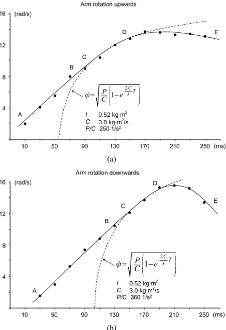
[image:6.595.56.287.154.301.2]curve A-E. The theoretical angular velocity function with maximum power hypothesis (Equation 15) was fitted into the curve of the measured angular velocity-time values. Moment of inertia of forearm rotation was calculated I = 0.11 kg·m2 (see 2.5). The values of friction coefficient C and power and friction coefficient ratio P/C were ob-tained within the curve fitting, C = 2.38 kg·m/s2 and P/C =285 1/s2. In Figure 5 the movement proceeds at a con-stant acceleration between the phases A and B (~ 40 - 80 ms) until the liquid friction begins to influence and ac-celeration decreases between B-C. According to the Hy-pothesis 2 the movement proceeds at a constant power between C-D which is followed by stopping of the movement (D-E). The theoretical angular velocity curve (broken line) coincides with the measured angular veloc-ity curve within section C-D. Therefore, we conclude that Hypothesis 2 is fulfilled within this range of velo- city.
Figure 7 represents the curves of the measured points of angular velocity-time values from the whole arm ro- tations downwards and upwards (Figure 6). The theo- retical angular velocity functions with maximum power hypothesis (Equation (15)) were fitted into the measured point curves. Moment of inertia of forearm rotation was calculated I = 0.52 kg·m2 (see 2.5). The values of friction coefficient C and power and friction coefficient ratio P/C were obtained within the curve fitting, whole arm rota-tion downwards C = 3.0 kg·m/s2 , P/C =360 1/s2 and whole arm rotation upwards C = 3.0 kg·m/s2, P/C =250 1/s2. The movement follows the hypothesized movement pattern described in the forearm rotation above. The theoretical angular velocity curves (broken lines) coin-cide with the measured angular velocity curves in section C-D (~ 150 - 190 ms and 90 - 150 ms in downward and upward rotation, respectively, Figure 7).
d d
I P C P I C
T T
(16)
yields one power value (P1) and the other one (P2) comes
from the curve fitting used in Figures 5 and 7 (P/C). In forearm rotation downwards the angular accelera- tion at point T = 0.10 s, = 14.5 rad/s was calculated by using the tangent of the angular velocity curve (Fig- ure 8). The tangent point can be found because the tan- gent has only one point on the curve, otherwise there are two intersection points. The value of angular acceleration in Figure 8 was calculated according to
d dT
= 14.5/0.12 1/s2 = 121 1/s2.
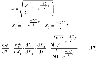
This value of angular velocity derivative can also be calculated using Equation (15). The time and angular velocity of this equation corresponding to the measured angular velocity curve time 0.10 s and velocity 14.5 rad/s was calculated with Equation (13). Substitution of veloc-ity 14.5 rad/s into Equation (13) gives time 0.031 s. The derivative of Equation (15)
1 2
2
2
1 ,
2 1 ,
CT
I
CT
I
P e C
C
X e X
I
T
2
1 2
1 2
2
2
d d
d d
d d d d
1
CT
I
CT
I
P C e
X X I
T X X T
e
(17)
Substituting in this equation T = 0.031 s, I = 0.11 kg·m2, C = 2.38 kg·m2/s and P = 693 W, the value of angular acceleration of 112 1/s2 was obtained. Moment arm of gravitational force is so short at forearm rotation that the power generation of gravitational force has no significance. In whole arm rotation downwards and whole arm rotation upwards the effect of gravitational force is within power P. The accuracy of results is pre-sented in Table 2.
4. Conclusions
[image:6.595.341.537.411.532.2]Angular acceleration dT
14.5 / 0.12 1/s 13 / 0.16 1/s 11 / 0.17 1/s
Moment of inertia (I) 0.11 kg·m2 0.52 kg·m2 0.52 kg·m2
Power into acceleration d d I
T
193 W 562 W 370 W
Coefficient of friction (C) 2.38 kg·m2/s 3.0 kg·m2/s 3.0 kg·m2/s
Power into friction
C2
500 W 531 W 363 WMuscle Power (P1) 693 W 1093 W 733 W
Power/Coefficient of friction (P/C) 285 1/s2 360 1/s2 250 1/s2
Muscle Power (P2) 678 W 1080 W 750 W
Error
11 22 100 0.5
P P P P
[image:7.595.55.537.113.496.2] 2.2% 1.2% 2.3%
Figure 8. Calculation of angular acceleration at point (T = 0.10 s, = 14.5 rad/s), where the theoretical angular ve-locity curve (broken line) coincides with the measured an- gular velocity curve (points) between C-D.
left side of Equation (8) is constant.
d d
P
I C
T
Torque accelerating the movement is not the same as muscle force which is included in the term P/. There- fore, we can conclude that Hypothesis 1 is not fulfilled. However, “movement proceeds at a constant accelera-tion” is an interesting finding which should be studied more closely. In Equation (8) kinetic friction was as- sumed to be directly proportional to velocity between A-B. This is a third hypothesis included into this study, which is not necessarily true. It is possible that kinetic
friction is constant at small velocities and at large veloci-ties directly proportional to velocity. Then there is a con- stant torque value accelerating the movement between A-B. The constant acceleration of the velocity curve may be related to the evolution of the human beings. For ex-ample the smooth acceleration may be essential for the accuracy of javelin throwing and targeting in fighting and hunting. As mentioned in [10] when modeling the control of the human limb motions, the final aim is to estimate the force production of individual muscles in-volved. Therefore the constant acceleration theory may play important role in human movements.
Hypothesis 2: movement proceeds at a constant maxi- mal muscle power. Since the matched range (C-D) of the theoretical and measured velocity curves of arm rotation was long enough, it can be clearly seen that the curves did not intersect each other. Therefore it can be inferred that the constant maximum power hypothesis is true be- tween C-D. In addition to the present study of three dif- ferent type of arm rotation experiments the model of constant maximum power was also fulfilled in the previ-ous experiments of shot put [11]. The different arm movements used in these experiments helped to achieve a greater certainty for the functioning ability of the pre-sent model. This model can be considered the most in-teresting finding of the present study.
REFERENCES
[image:7.595.56.309.116.507.2][4] W. Herzog, “Mechanical Properties and Performance in Skeletal Muscles,” In: V. Zatsiorsky, Ed., Biomechanics in sport, Blackwell Science University Press, Cambridge, 2000, pp. 21-32. doi:10.1002/9780470693797.ch2
[5] B. R. MacIntosh and R. J. Holash, “Power Output and Force Velocity Properties of Muscle,” In: B. M. Nigg, B. R. MacIntosh and J. Mester, Eds., Biomechanics and Bi-ology of Movement, Human Kinetics, Champaign, 2000, pp. 193-210.
[6] D. A. Winter, “Biomechanics and Motor Control of Hu-man Movement,” 3rd Edition, John Wiley & Sons Inc., Hoboken, 2004, pp. 215-222.
[7] J. H. Challis, “Muscle-Tendon Architecture and Athletic performance,” In: V. Zatsiorsky, Ed., Biomechanics in sport, Blackwell Science University Press, Cambridge, 2000, pp. 33-55. doi:10.1002/9780470693797.ch3
[8] D. E. Rassier, B. R. MacIntosh and W. Herzog, “Length Dependence of Active Force Production in Skeletal Mus-cle,” Journal of Applied Physiology, Vol. 86, No. 5, 1999,
[10] R. T. Raikova and H. Ts. Aladjov, “Comparison between Two Models under Dynamic Conditions,” Computers in Biology and Medicine, Vol. 35, No. 5, 2005, pp. 373-387.
doi:10.1016/S0010-4825(04)00041-1
[11] A. Rahikainen and P. Luhtanen, “A Study of the Effect of Body Rotation on the Arm Push in Shot Put,” Russian Journal of Biomechanics, Vol. 8, No. 2, 2004, pp. 78-93. [12] A. Rahikainen, “Biomechanics in Shot Put,” Helsinki
University, Helsinki, 2008.
[13] A. Rahikainen, J. Avela and M. Virmavirta, “Modeling the Force—Velocity Relationship in Arm Movement,” Proceedings of the 14th ECSS Congress, Oslo, 24-27 June 2009, p. 570.
[14] A. Rahikainen, “Method and Apparatus for Photograph-ing a Movement,” US Patent No. 4927261, 1990. [15] A. Rahikainen, “The Use of Rotating Disk in the