Mineral Prospectivity Mapping Method Integrating Multi Sources Geology Spatial Data Sets and Case Based Reasoning

Mineral Prospectivity Mapping Method Integrating

Multi-Sources Geology Spatial Data Sets and

Case-Based Reasoning

Binbin He1, Jianhua Chen2, Cuihua Chen3, Yue Liu3

1_{School of Resources and Environment, University of Electronic Science and Technology of China, Chengdu, China} 2_{College of Geophysics, Chengdu University of Technology, Chengdu, China}

3_{College of Geosciences, Chengdu University of Technology, Chengdu, China}

Email: binbinhe@uestc.edu.cn, {chjh3, chencuihua}@163.com

Received October 26,2011; revised December 20, 2011; accepted January 4, 2012

ABSTRACT

Extracting and synthesizing information from existing and massive amounts of geology spatial data sets is of great sci-entific significance and has considerable value in its applications. To make mineral exploration less expensive, more efficient, and more accurate, it is important to move beyond traditional concepts and establish a rapid, efficient, and intelligent method of predicting the existence and location of minerals. This paper describes a case-based reasoning (CBR) method for mineral prospectivity mapping that takes spatial features of geology data into account and offers an intelligent approach. This method include a metallogenic case representation that combines spatial and attribute features, metallogenic case-based storage organization, and a metallogenic case similarity retrieval model. The experiments were performed in the eastern Kunlun Mountains, China using CBR and weights-of-evidence (WOE), respectively. The re-sults show that the prediction accuracy of the CBR is higher than that of the WOE.

Keywords: Mineral Prospectivity Mapping; Case-Based Reasoning; Metallogenic Case Representation; Metallogenic Case Retrieval; Eastern Kunlun Mountains

1. Introduction

Mineral prospectivity analysis and quantitative resource estimation have been recognized as important when inte-grating multi-source geology spatial data in recent years [1]. The statistical and mathematical approaches devel-oped recently for multi-resources geological spatial data integration include weights-of-evidence (WOE) [2-8], and the logistic regression [9,10]. The fuzzy logic [11, 12], artificial neural networks [13,14] and the Fractal method [15] have been applied in the assessment of min-eral resources potential. Although these methods promote the efficiency and effectiveness of mineral resource prospecting, their algorithms are unable to accumulate knowledge, and lack intelligent reasoning. Meanwhile, similar deposit types occur in similar geological condi-tions and spatial distribucondi-tions. The metallogenic geo-logical conditions and spatial distribution of discovered and typical deposits can be used to construct a historical case-base for mineral prospectivity analysis. Traditional analysis methods cannot mine the depth of information or make intelligent inferences. In recent years, some re-searchers have begun applying case-based reasoning (CBR) to the environment, urban planning, and land use.

provement of efficiency and quality, and the accumula- tion of knowledge. Additionally, CBR and the identifica- tion process are highly automated and reusable. CBR is an effective method in cases in which prior knowledge is lacking or for constructing complex issues in quantitative models.

In this paper, a method for mineral prospectivity map-ping was proposed integrating multi-sources geology spatial data sets and case-based reasoning, including a metallogenic case representation model that combines spatial and attribute features, the metallogenic case-fea- ture weights-determining model, metallogenic case-based storage organisation, and a metallogenic case-similarity retrieval model. The experiment was performed in the eastern Kunlun Mountains, China to predict the existence of potential iron deposits using case-based reasoning and weights-of-evidence, respectively.

2. Methodology

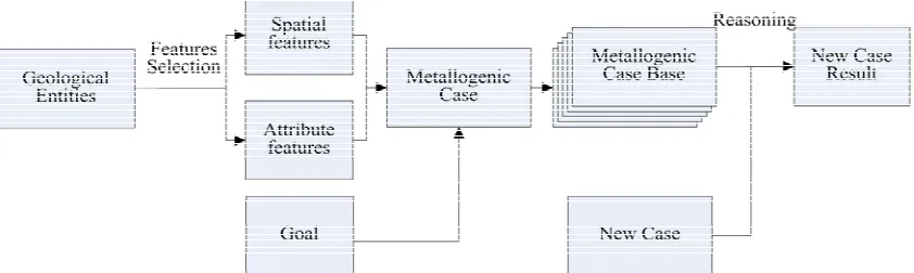
The mineral prospectivity mapping method using case- based reasoning include three main components: a met- allogenic case representation model, metallogenic case storage, and a metallogenic case retrieval model. Figure 1 describes the flow of mineral prospectivity mapping method using CBR.

2.1. Metallogenic Case Representation Model

Generally, a case in a traditional CBR model is com- posed of both attribute and goal features. Because of the spatial distribution and regional laws of geological enti- ties, the case representation is different from a traditional one. The features of a metallogenic case include both spatial and attribute features, which are selected or ex- tracted from metallogenic entities.

During the construction of a metallogenic case repre- sentation model, each grid of a certain size is taken as a representative object. First, typical feature attributes re-lated to ore control that are contained in vector grids of existing mineral points are extracted. Then, the corre- sponding names of mines in vector grids and relevant

result values are determined. The extracted-features at- tribute, the corresponding names, and the relevant results are all described by the rules of case expression. To ex- tract spatial features, the orientation relations, the metric relations, and the topology relations related to ore control in each vector grid are extracted, and spatial relations are transformed to attribute mode. Therefore, a metallogenic case consists of general attributes and spatial-relation property items. The basic expression is as follows:





C A A  A A A A (1)

where Aai is the general feature property item, Asj is the

spatial-relation feature property item, and Result repre-sents the result of the case. To solve a new case, existing cases can be extracted by spatial relations under certain rules (e.g., spatial coding). After that, candidates for a historical case set are obtained.

2.2. Metallogenic Case Storage

After a typical metallogenic case is constructed, it is stored in a spatial database in database tables or into document systems in a text file. The stored cases are then indexed to improve the efficiency of the metallogenic case-similarity retrieval model.

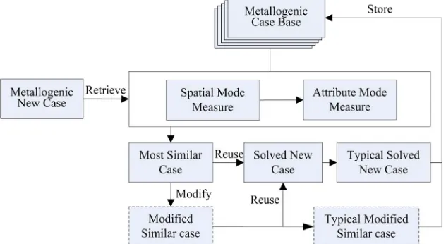
2.3. Metallogenic Case Retrieval Model

Because a metallogenic case has spatial features, it is different than a traditional CBR model. First, during the construction of a metallogenic case retrieval model, all vector grids are set as unsolved cases under the metal- logenic case representation model. In other words, each case describes typical attribute and spatial features, and the results description (i.e., the case-determining attribute) is set to blank. Second, a similarity-measure threshold is set, and each unsolved case is retrieved for similarity. After a similar case is found, its result is assigned to the unsolved case according to the threshold and the strategy given. If the case obtained is unsatisfactory, it can be modified by expertise. Its result can then be assigned to the unsolved case. The retrieval unsolved cases in all

vector grids are then completed. Third, the typical cases obtained or modified can be stored into the case base for expansion and update.

After a metallogenic case base is constructed, the met- allogenic case retrieval model (Figure 2) can use it to compare existing metallogenic cases with new ones. The similarity measurement formulas for existing and new cases are as follows:

%

di 100* 1 sqrt

sum(

searchedWeightsS *

totalWeightsSum S _  

  stance weights) um        _{ }  _       2 2 2 2 2 eight *dist ist n n



distance weight *dist w weight *d

 

  (3)







dist

diff newCaseValue, caseValue min 1,

maxValue minValue *inf inityCons tant

 

 

 _ 

 

(4)

where “S%” is similarity ranged between 0% and 100%;

“distance” is the weighted sum of the squares of “disti”

ranged between 0 and 1; “searchedWeightsSum” is the sum of the weights, with the new case feature and the actual case feature both being non-empty; “totalWeig- htsSum” is the sum of the weights of all case features; “disti” is the distance between the new case feature and

the actual case feature, in which the value is the smaller of either 1 or the Euclid distance between the new case feature and the actual case feature; “newCaseValue” is the new case feature value; “caseValue” is the actual case feature value; “maxValue” and “minValue” are the case corresponding feature’s maximum and minimum values; and “infinityConstant” is a large constant.

To measure similarity, each new case is compared with

all cases in the case base. The return value is based on the selection strategies of the maximum, threshold, or K nearest neighbors. If the value is unsatisfactory, it can be modified by the return value and relevant expertise. The typical cases obtained and the cases modified can be stored into the case base for expansion.

3. Experiments

To verify the effectiveness of the proposed method, the experiments of mineral potential prediction for iron de- posits were performed in the eastern Kunlun Mountains, using the metallogenic CBR model and the weights-of- evidence model, respectively. All of the data sets used in this paper were derived from our established multisource geology spatial database, which contains geological, geophysical, geochemical, and remote-sensing data. The metallogenic CBR model was implemented with C# _based

on ArcEngine GIS components. The weights-of-evidence model was performed with Arc-SDM [21].

3.1. Geological Setting of Study Area

The eastern Kunlun Mountains are within Qinghai Prov- ince, China, and are shown as an insertion from left to right to the provincial map (Figure 3). The Mountains are within latitudes 34˚57′ and 37˚56′N, and longitudes 90˚31′ and 100˚04′E. Of the study area, the eastern Kun- lun orogenic belt is attached to the southern margin of the Qaidam Basin.

The area consists of three major deep crustal-scale faults that divide the area roughly from north to south into sub- tectonic belts (Figure 4). Kunbei (“Kun” is short for Kunlun. “bei” means north in Chinese) belt is in the north. It belongs to the Kunbei Caledonian back-arc basin situ-ated mainly in the northwestern part of the Kunlun Mountains. The belt is made of early Palaeozoic folding belts dominated by the Ordovician marine sediments

Figure 3. Eastern Kunlun Mountains within Qinghai Province, China.

Note: Showing major lithologic units, stratigraphic units, and crustal-scale faults. The east Kunlun orogenic belt is subdivided into the Kunbei belt, and the Kunnan belt.

and low-grade metamorphic rock. Kunzhong (“zhong” is middle in Chinese) belt is the basement of an uplift belt and a granitic belt. It is made predominantly of the mid- dle to late Proterozoic metamorphic sequences, and Pa- laeozoic and Mesozoic granitic rock. The Devonian con- tinental sandstones, conglomerate, and volcanic rock, and Carboniferous marine limestone and sedimentary rock lie over the metamorphic and plutonic basement. The com- position of Kunnan (“nan” means south in Chinese) belt is geologically similar to that of the Kunzhong belt, but it consists of numerous Triassic successions. As of today, there are 81 known sites of iron formation within the area. Their locations are shown as black dots in Figure3.

Within the study area, regions exposed mainly by lithologic and stratigraphic units are displayed in Figure 4. The Jinshuikou Group is the oldest crystalline base- ment that comprises gneiss, amphibolite rock, migmatite, and marble. It belongs to a suite of middle-to-high grade of metamorphic rock [22]. The Tanjianshan Group of the Ordovician-Cambrian period is composed of intermedi- ate-mafic volcanic rock, and phyllite crystalline limestone and sandstone. The Elashan Formation of the Triassic time consists basically of volcanic rock that is intermedi- ate-acid. The rock is with sandstone intercalation. The Wanbaogou Group of the New Mesoproterozoic period is subdivided into an upper unit and a lower one, compris- ing mainly carbonate rock and intermediate-mafic vol- canic rock. Both types of rock belong to the pre-Cambrian folding basement with a low-grade of metamorphism [23]. The volcanic rock and carbonaceous slate of the Wanbaogou Group serve as important ore beds of pre- cious metal (e.g., gold) and non-ferrous metals (copper, cobalt, and nickel) in the Kunnan belt [24]. The Nachitai Group of the Ordovician period consists largely of schist, mafic volcanic rock, chert, and crystalline limestone. The Maoniushan Formation of the Devonian time is com- posed of an intermediate-acid volcanic rock underlain by clastic rock. The Variscan-Indosinian granite is closely associated with the metalliferous mineralization in the region when the granite occurs extensively, diversely and permanently [25]. Known iron mineralization occurred mainly in the Yemaquan metallogenic belt located in the western part of the Mountains, whereas the Dulan-Elashan metallogenic belt lies in the east.

3.2. Data Preprocessing and Metallogenic Case Construction

The best ore-controlling variable and threshold were de- termined using proximity analysis of the weights-of- evidence model. On the basis of a correlation analysis among evidence variables, the authors selected vector ore-controlling data of stratum, unconformity, fault, re- gional geochemical data, remote-sensing mineralization information, Bouguer gravity data, aeromagnetic data,

and mineral occurrence for this experiment. Before con- structing the specific metallogenic case, the region was partitioned into 96,576 grids, each one being 1 km by 1 km. All of the evidence-variable data were spatially joined to a grid polygon, and each grid had corresponding fea-ture-attribute values. The unconformity, fault, and min-eral occurrences were buffered by with distances of 3000 m, 300 m, and 1000 m, respectively.

To extract the spatial features of the metallogenic case, the fault’s direction (orientation relationship), the short- est distance between mineral occurrence and faults (met- ric relationship), the disjoint relationship between min- eral occurrence and faults, and the unconformities (to- pology relationship) were computed and extracted in each grid polygon. The spatial relationships were then transformed into attributes and stored in the attribute tables of each grid polygon. This process paved the way for metallogenic case retrieval. In this way, the metal- logenic representation model combined with spatial and attribute features was constructed. Each grid polygon became a case representation object. By analyzing each grid layer’s attribute table in tandem with ore-controlling factors, the authors established the metallogenic case’s attribute features by using lithological characters, chro- nostratigraphy, unconformity, fault, regional chemical ano- maly, remote-sensing mineralisation anomaly, Bouguer gravity anomaly, and aeromagnetic anomaly. In this way, specific genetic types became object attributes. The met- allogenic case representation model in this research is as follows:

C = (unconformity, regional geochemical anomaly, Bouguer gravity anomaly, aeromagnetic anomaly, chro- nostratigraphy, lithological characters, remote-sensing mineralisation anomaly, fault characters, fault directions, short distance to fault, distance to unconformity, disjoint fault, disjoint unconformity, genetic type).

Prior to analysis, the attribute and spatial features of the above case are set corresponding weights, which are determined and assigned based on the Analytic Hierarchy Process (AHP) [26]. On the basis of expert knowledge, the importance of AHP case features is as follows: re- gional geochemical anomaly > fault directions > short distance to fault = disjoint fault > fault characters = re-mote-sensing mineralisation anomaly > chronostratigra-phy = lithological characters > distance to unconformity = disjoint unconformity > unconformity characters = Bouguer gravity anomaly = aeromagnetic anomaly. Ta-ble 1 shows the comparison matrix of metallogenic CBR features by AHP. The matrix is equalised and simplified to seven features. After calculating, uniformity has been passed and each feature weight determined; identical, important features have the same weights (Table 2).

Table 1. The CBR features comparison matrix by AHP.

B1 B2 B3 B4 B5 B6 B7 B8 B9 B10 B11 B12 B13 B1 1 1/7 1 1 1/3 1/3 1/4 1/4 1/6 1/5 ½ 1/5 1/2

B2 1 7 7 7/3 7/3 7/4 7/4 7/6 7/5 7/2 7/5 7/2

B3 1 1 1/3 1/3 1/4 1/4 1/6 1/5 ½ 1/5 1/2

B4 1 1/3 1/3 1/4 1/4 1/6 1/5 ½ 1/5 1/2

B5 1 1 3/4 3/4 3/6 3/5 3/2 3/5 3/2

B6 1 3/4 3/4 3/6 3/5 3/2 3/5 3/2

B7 1 1 4/6 4/5 4/2 4/5 4/2

B8 1 4/6 4/5 4/2 4/5 4/2

B9 1 6/5 6/2 6/5 6/2

B10 1 5/2 1 5/2

B11 1 2/5 1

B12 1 5/2

B13 1

B1: unconformity; B2: regional geochemical anomaly; B3: Bouguer gravity anomaly; B4: aeromagnetic anomaly; B5: chronostratigraphy; B6: lithological characters; B7: remote-sensing mineralisation anomaly; B8: fault characters; B9: fault directions; B10: short distance to fault; B11: distance to unconformity; B12:disjoint fault; B13:disjoint unconformity.

Table 2. The CBR equivalent property features comparison matrix and weights determined by AHP.

B1 B2 B3 B4 B5 B6 B7 Weights

B1 1 7 7/3 7/4 7/6 7/5 7/2 0.250

B2 1 1/3 ¼ 1/6 1/5 1/2 0.036

B3 1 ¾ 3/6 3/5 3/2 0.107

B4 1 4/6 4/5 4/2 0.143

B5 1 6/5 6/2 0.214

B6 1 5/2 0.179

B7 1 0.071

B1: regional geochemical anomaly; B2: Bouguer anomaly; B3: chronostratigraphy; B4: remote-sensing mineralization anomaly; B5: fault directions; B6: short distance to fault; B7: distance to unconformity.

layer’s attribute table, selected all the records in which the field showing the genetic type of mineral occurrence was non-empty, and exported those records for further analysis. The final records were stored in a text file in which all attribute values were separated by tabs. The corresponding genetic type case base was then con- structed. The attribute tables of relevant grid polygon layers were exported and stored in a text file, and each unsolved case set was constructed (each grid represents an unsolved case object). Each grid in the polygon layers corresponds to an unsolved metallogenic case. After a similarity measurement, each grid was assigned a genetic type, and the similarities were assigned values between 0 and 100%. In this way, the classification strategy auto- matically outlined a regional metallogenic prediction map showing high, medium, and low potentials.

3.3. Mineral Potential Prediction Results and Analysis

Based on the data-processing and metallogenic CBR model

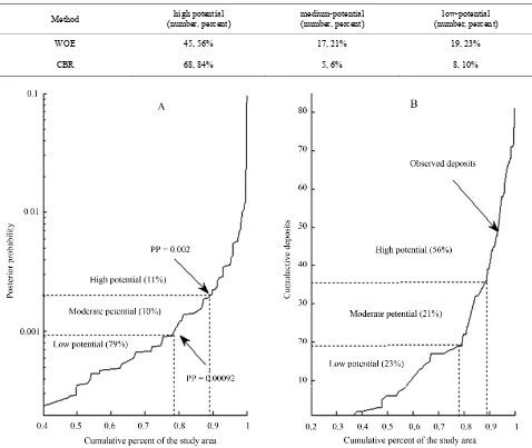
described above, an experiment regarding mineral poten-tial prediction for iron deposits was performed in the eastern Kunlun Mountains, China. Figure 5 reports, re-spectively, the curves representing the relationships be-tween 1) posterior probability based on the WOE and cumulative mineral occurrence; and 2) posterior prob-ability and cumulative areas. Table 3 and Figure 6 show the favorable metallogenic potential regions (i.e., areas of high and medium potential) extracted using weights-of- evidence model. High- and medium-potential areas oc-cupy 21% of the study area and contain 62 points of 81 known deposit points (i.e., 77% of known deposit points). High-potential areas occupy 11% of the total area and include 45 known deposit points (i.e., 56% of known de- posit points). Medium-potential areas occupy 10% of the total area and include 17 known deposit points (i.e., 21% of known deposit points).

Table 3. The contrast of prediction results using CBR and WOE.

Method _{(number, percent)} high potential medium-potential _{(number, percent) (number, percent)} low-potential

WOE 45, 56% 17, 21% 19, 23%

CBR 68, 84% 5, 6% 8, 10%

Figure 5. Variation of cumulative area with sum of weights and cumulative deposits using WOE.

Figure 7. Potential prediction map for iron deposits using CBR in eastern Kunlun Mountains, China.

study area, with high-potential areas accounting for 10% of the total area and the medium-potential areas accounting for 11% of the total area. The prediction results show that known mineral occurrence is highly consistent with the high-potential areas, as analysis predicts that 68 of 81 known mineral occurrences fall into the high-potential areas (84%), 5 fall into the medium-potential areas (6%), and 8 fall into the low-potential areas (10%). Overall prediction accuracy (high- and medium-potential areas account for 90%) is significantly higher than the accu-racy of the traditional weights-of-evidence model (i.e., 77%).

4. Conclusion

The metallogenic CBR method for regional mineral pros- pectivity mapping is a new and intelligent prediction method. It makes full use of multisource massive geol- ogy spatial data. It also surpasses traditional mineral- prediction approaches to improve the intelligence, effi- ciency, and accuracy of mineral prediction. This paper takes spatial features of geology data into account and proposes an integral metallogenic CBR method, which includes the metallogenic case representation model, metallogenic case storage, and the metallogenic case similarity retrieval model. Finally, an application of mineral potential pre- diction for iron deposits was performed in the eastern Kunlun Mountains, China, using a metallogenic CBR and WOE, respectively. The results indicated that the predic-tion accuracy of the metallogenic CBR is significantly higher than the accuracy of the traditional weights-of-evi- dence model.

5. Acknowledgements

This study was supported by the National Natural Science Foundation of China (Grant No. 41171302 & 40701146) and the National High-Tech R&D Program of China

(Grant No. 2007AA12Z227). We express our gratitude to Zhuang Yongcheng from the Qinghai Institute of Geol-ogy Survey for his directions.

REFERENCES

[1] A. K. Porwal and O. P. Kreuzer, “Introduction to the Special Issue: Mineral Prospectivity Analysis and Quan- titative Resource Estimation,” Ore Geology Reviews, Vol. 38, No. 3, 2010, pp. 121-127.

doi:10.1016/j.oregeorev.2010.06.002

[2] G. F. Bonham-Carter, F. P. Agterberg and D. F. Wright, “Weights of Evidence Modeling: A New Approach to Mapping Mineral Potential,” In: F. P. Agterberg, et al., Eds., Statistical Applications in the Earth Sciences, Ca- nadian Government Publishing Centre, Ottawa, 1989, pp. 171-183.

[3] F. P. Agterberg, “Combining Indicator Patterns in Weights of Evidence Modeling for Resource Evaluation,” Natural Resources Research, Vol. 1, No. 1, 1992, pp. 39-50. doi:10.1007/BF01782111

[4] J. R. Harris, L. Wilkinson and E. C. Grunsky, “Effective Use and Interpretation of Lithogeochemical Data in Re- gional Mineral Exploration Programs: Application of Geo- graphic Information Systems (GIS) Technology,” Ore Geology Reviews, Vol. 16, No. 3-4, 2000, pp. 107-143.

doi:10.1016/S0169-1368(99)00027-X

[5] E. J. M. Carranza, “Weights of Evidence Model of Min-eral Potential: A Case Study Using Small Number of Prospects, Abra, Philippines,” Natural Resources Re-search, Vol. 13, No. 3, 2004, pp. 173-187.

doi:10.1023/B:NARR.0000046919.87758.f5

[6] B. Daneshfar, A. Desrochers and P. Budkewitsch, “Min-eral-Potential Mapping for MVT Deposits with Limited Data Sets Using Landsat Data and Geological Evidence in the Borden Basin, Northern Baffin Island, Nunavut, Can- ada,” Natural Resources Research, Vol. 15, No. 3, 2006, pp. 129-149. doi:10.1007/s11053-006-9020-7

Cuaig and A. Mamuse, “Weights-of-Evidence and Logis- tic Regression Modeling of Magmatic Nickel Sulfide Pros- pectivity in the Yilgarn Craton, Western Australia,” Ore Geology Reviews, Vol. 38, No. 3, 2010, pp. 184-196. doi:10.1016/j.oregeorev.2010.04.002

[8] B. B. He, C. H. Chen and Y. Liu, “Gold Resources Poten-tial Assessment in Eastern Kunlun Mountains of China Combining Weights-of-Evidence Model with GIS Spatial Analysis Technique,” Chinese Geographical Science, Vol. 20, No. 5, 2010, pp. 461-470.

doi:10.1007/s11769-010-0420-6

[9] F. P. Agterberg, G. F. Bonham-Carter, Q. M. Cheng and D. F. Wright, “Weights of Evidence Model and Weighted Logistic Regression in Mineral Potential Mapping,” In: J. C. Davis, et al., Eds., Computers in Geology, Oxford Uni- versity Press, New York, 1993, pp. 13-32.

[10] E. J. M. Carranza and M. Hale, “Logistic Regression for Geologically Constrained Mapping of Gold Potential, Ba- guio District, Philippines,” Exploration and Mining Ge-ology, Vol. 10, No. 3, 2001, pp. 165-175.

doi:10.2113/0100165

[11] F. Aminzadeh, “Applications of Fuzzy Expert Systems in Integrated Oil Exploration,” Computers & Electrical En- gineering, Vol. 20, No. 2, 1994, pp. 89-97.

doi:10.1016/0045-7906(94)90023-X

[12] X. Luo and R. Dimitrakopoulos, “Data-Driven Fuzzy Ana- lysis in Quantitative Mineral Resource Assessment,” Com- puters & Geosciences, Vol. 29, No. 1, 2003, pp. 3-13.

doi:10.1016/S0098-3004(02)00078-X

[13] K. Koike, S. Matsuda, T. Suzuki and M. Ohmi, “Neural Network-Based Estimation of Principal Metal Contents in the Hokuroku District, Northern Japan, for Exploring Ku- roko-Type Deposits,” Natural Resources Research, Vol. 11, No. 2, 2002, pp. 135-156.

doi:10.1023/A:1015520204066

[14] J. P. Rigol-Sanchez, M. Chica-Olmo and F. Abarca-Her- nandez, “Artificial Neural Networks as a Tool for Mineral Potential Mapping with GIS,” International Journal of Remote Sensing, Vol. 24, No. 5, 2003, pp. 1151-1156. doi:10.1080/0143116021000031791

[15] P. Gumiel, D. J. Sanderson, M. Arias, S. Roberts and A. Martín-Izard, “Analysis of the Fractal Clustering of Ore Deposits in the Spanish Iberian Pyrite Belt,” Ore Geology Reviews, Vol. 38, No. 4, 2010, pp. 307-318.

doi:10.1016/j.oregeorev.2010.08.001

[16] G. P. Lekkas, N. M. Avouris and L. G. Viras, “Case- Based Reasoning in Environmental Monitoring Applica-tions,” Applied Artificial Intelligence, Vol. 8, No. 3, 1994, pp. 359-376. doi:10.1080/08839519408945448

[17] A. Holt and G. L. Benwell, “Applying Case-Based Rea-soning Techniques in GIS,” International Journal of Geographical Information Science, Vol. 13, No. 1, 1999, pp. 9-25. doi:10.1080/136588199241436

[18] J. A. Ye and X. Shi, “Integrating Case-Based Reasoning and GIS for Handling Planning Applications,” Journal of Urban Planning Department, No. 3, 2001, pp. 34-40. [19] Y. Y. Du, W. Wen, F. Cao and J. Min, “A Case-Based

Reasoning Approach for Land Use Change Prediction,” Expert Systems with Applications, Vol. 37, 2010, pp. 5745-5750. doi:10.1016/j.eswa.2010.02.035

[20] R. C. Schank and P. A. Robert, “Scripts, Plans, Goals, and Understanding: An Inquiry into Human Knowledge Structures,” Lawrence Erlbaum, Hillsdale, 1977.

[21] L. D. Kemp, G. F. Bonham-Carter and G. L. Raines, “Arc- WofE: ArcView Extension for Weights of Evidence Map- ping [EB/OL],” 1999.

http://gis.nrcan.gc.ca/software/arcview/wofe

[22] G. C. Wang, Q. H. Wang, P. Jian and Y. H. Zhu, “Zircon SHRIMP Ages of Precambrian Metamorphic Basement Rocks and Their Tectonic Significance in the Eastern Kunlun Mountains, Qinghai province, China,” Earth Sci-ence Frontiers , Vol. 11, No. 4, 2004, pp. 481-490 . [23] Y. S. Pan, W. M. Zhou and R. H. Xu, “The Early

Palao-zoic Geological Features and Evolutions of the Kunlun Mountain,” Science in China (Series D), Vol. 26, No. 4, 1996, pp. 302-307.

[24] X. D. Guo, Y. J. Zhang, G. G. Liu, A. J. Pan and F. Zhang, “Metallogenic Regularities and Prospecting Di- rection of Gold and Copper in Eastern Kunlun,” Gold Geology, Vol. 10, No. 4, 2004, pp. 16-22.

[25] Z. Z. Qian, Z. G. Hu, J. Q. Liu and H. M. Li, “Active Con- tinental Margin and Regional Metallogenesis of the Pa- laeo-Tethys in the East Kunlun Mountains,” Geotectonica et Metallogenia, Vol. 24, No. 2, 2000, pp. 134-139. [26] T. L. Saaty and L. G. Vargas, “Uncertainty and Rank Or-