ISSN Online: 2152-7261 ISSN Print: 2152-7245
A Model of the Market Process with Numerical
Simulation
Ricardo Luis Chaves Feijó, Fabio Barbieri
School of Economics, Business Administration and Accounting at Ribeirão Preto, University of São Paulo, São Paulo, Brazil
Abstract
The paper simulates the price-arbitrage process at the market for homogene-ous good and tries to show the convergence into a single price from different cross-linked markets of this homogeneous good. It examines the problem by random generation of values in the simulation environment offered by the Matlab program. It is emphasized here the approach in which the agent’s alertness is crucial to the market. The emphasis is not on the price that equilibrates supply and demand, since there is not a single price for a homo-geneous commodity. A homohomo-geneous good is negotiated with different prices in different parts of a market. The paper explains the process in which the agent’s alertness leads to a uniform price in terms of a simulation model, in the belief that that technique leads to a better understanding of the precise nature of the market process and the agent’s alertness role in equilibration. The paper also discusses the effects of the heterogeneous agents and market barriers in the market convergence process. The innovative feature of the pa-per is the simulation expa-periment.
Keywords
Numerical Simulation, Alertness, Market Process
1. Introduction
Two main pointes make us believe that the paper has the potential to contribute to the literature. First, numerical simulations seem to be a fruitful way to study market process and price convergence, in particular. Second, the inclusion of alertness itself as a determinant of the probability of discovery of new markets is an interesting and novel assumption.
Forty-eight years ago, Littlechild and Owen [1] developed an algebraic model to describe the market process. They claimed to be the mathematical formalization How to cite this paper: Feijó, R.L.C. and
Barbieri, F. (2018) A Model of the Market Process with Numerical Simulation. Mod-ern Economy, 9, 1868-1897.
https://doi.org/10.4236/me.2018.911118
Received: October 2, 2018 Accepted: November 17, 2018 Published: November 20, 2018
Copyright © 2018 by authors and Scientific Research Publishing Inc. This work is licensed under the Creative Commons Attribution International License (CC BY 4.0).
http://creativecommons.org/licenses/by/4.0/
Open Access
of the Austrian school’s view of the market process. However, such a model dis-torts the fundamental meaning of the Austrian dynamics approach on market. It does not faithfully follow Ludwig von Mises’s approach to the market process, it is not faithful to the concept of equilibrium of this school (logical equilibrium and not mathematical one), it does not describe the price mechanism as Aus-trian economists do, does not effectively address the role of the entrepreneurial activity on the functioning of the markets.1 In short, though pioneering, it had been a failed attempt to give Austrian insights a mathematical treatment.2
Nevertheless, the structure of the model developed in the pioneer paper allows an interesting computational approach to the process of price arbitrage in the markets for a homogeneous good. In particular, it is important to show the pos-sibility of converging to a single price for the good in question when the markets are initially isolated from one another and are gradually linked by the agents’ own arbitration process, as they discover these markets and those are integrated with each other.
The idea that arbitrage would bring about a single price for homogeneous good is very old in economic thought.3 The intuition, widely disseminated in the profession, is that the quotations of homogeneous goods converge quickly at a single price by the agents’ action in the market. However, in the last century the scientific community has more technically examined the problem of uniform price formation in the markets and concluded that the process would not be so simple and immediate. In fact, a gigantic literature on learning (in particular prices) is accumulating, including decision errors and limited rationality. In ad-dition, the growing treatment of the problem by computational methods and numerical simulation procedures is noted.4
In this spirit, we propose an interesting and original treatment of the basic problem of simultaneous price convergence of a homogeneous good practiced in different markets by means of random generation of values of the variables in the simulation environment offered by the Matlab program.5 The hypotheses of the new treatment are simple and follow in general the model of Littlechild and Owen, although with no pretense of being an Austrian representation of the market process. The point of advancement in relation to the pioneer model is the possibility of a probabilistic treatment of the process of discovery of new 1Lundholm [2] believes that the theoretical model in question uses only the initial ideas of Kirzner, an Austrian school economist, as Kirzner [3] does, and it does not quite describe the author’s in-sights after 1982 when he incorporates more fundamentally the role of uncertainty. According to the critic, the model, in fact, is not tied to the more recent Austrian description of the market process in which agents discover individual buyers and sellers, not markets. See Kirzner [4].
2According to the Google Scholar indicator, the paper was cited 41 times since, scientific perfor-mance short of a successful study. Moreover, it is noted that it was published in a highly regarded journal (Journal of Economic Theory). Although there is much more mathematics today in Austrian models than in the past, the paper in question did not have the repercussion that was imagined. 3It was present in the classical economists, and Alfred Marshall reiterated it.
4In general, these studies are based on a modeling structure with game theory. Keyhani [5] offers an interesting survey of numerical simulation procedures investigating price convergence.
5Computer simulations allow us to go beyond analytical treatment and to study systems that cannot be easily modeled with equations.
markets, or of new prices, through computational simulation exercises. Purely algebraic treatment and the corresponding price convergence theorems in dif-ferent markets for a homogeneous good are not successful in incorporating into the equations the process of market discovery itself and their integration through arbitrage. In fact, such a process is only presupposed, and not demon-strated or evaluated as to its effectiveness; the speed of integration given the mechanism of discovery etc. The use of simulation, instead of mathematical analysis, allows a detailed study, though artificial data, of the dynamics of con-vergence taking into account the discoveries by the agents of new prices.
It is, therefore, a study on the role of knowledge and discovery in the process of price convergence in the markets; a relevant study even if, over time, the sin-gle convergence price is not necessarily the intertemporal equilibrium price. The single price obtained by the arbitrage of the markets, accompanied by increasing discoveries by the agents, would not be a final state for the price practiced in the
linked markets (effectively arbitrated by a common set of agents). The study of uniform price formation, however, facilitates the investigation of the equilibrium price by allowing a single price to be assigned subsequently to each homogene-ous good. In this setting, one can study the possibility that the traditional condi-tions of general equilibrium be met.
The central contribution of the essay lies in the use of computational simula-tions to model the discovery of new markets through a probabilistic process that controls the agent’s chance to discover a market, starting from its base, the place where he previously knows and arbitrates, by a distribution of probabilities whose variance depends on a particular propensity of the agent in question, his alertness.6
Although there is an enormous amount of studies dealing with the process of convergence of markets by discovery of new prices, we did not find any numeri-cal simulation study with the use of a simple Matlab program and able to study the effectiveness of the convergence process and its sensitivity to the basic para-meters of the model. When the problem of incomplete information in which economic agents operate is recognized, the traditional approach focuses more on the restrictive role of imperfect information and the costs of obtaining informa-tion. The genuinely Austrian approach incorporates a radical ignorance of the agents, which is not quantifiable, which is unknown to the analyst, and therefore very difficult to model. More than just assuming that agents are unaware of formation sets, Austrians are concerned with studying the process by which in-formation is revealed to agents and how they learning to interpret it. From this point of view, the discovery of information involves surprise and could not be priced. Economists at the Austrian school investigate to what extent and under 6The term refers to the concept widely used by Kirzner ([3], [6]), which in this author is much richer and full of implications. It concerns the entrepreneur’s role in discovering opportunities and how this leads to market equilibrium. In this explanation, entrepreneurial activity is crucial for the mar-ket process to equilibrium. The concept of alertness in Kirzner also incorporates speculative and in-novative activities.
what conditions such a discovery would lead the market toward equilibrium. In the real and complex economy, they ask whether there is a tendency to approach, rather than distancing, the equilibrium trajectory.
The proposed simulation model sheds new light on the process in which equi-librium is reached, with reference to a formal model that follows many aspects of pioneering treatment, however, with no pretense of formalizing the richness of the Austrian approach. It is only a model of numerical simulation of the process of convergence of prices in the markets. The emphasis is only on the arbitration process. At every moment, the price adjustment in each market obeys the law of supply and demand, and the interest is only in how different prices converge with the gradual integration of the markets by the agents’ arbitrage. Therefore, the emphasis of the study falls not on the concept of equilibrium itself, but on the mechanism of equilibration. A homogeneous good is transacted at different prices in different parts of a market because the market participant does not know all of it (knows only parts of it or submarkets). It is imagined here that, with the discovery of the agents, given the alertness of each one, a uniform price is arrived at. Given the price differences between the new market and the known markets, transfers of goods take place immediately. There is no lag between buying and selling in the model, within which prices could change. This price can, after being reached, be examined regarding its dynamic stability by a gener-al equilibrium model, which does not belong to the scope of this study. It is then a question of providing a description of the process of price convergence in terms of a simulation exercise based on a mathematical model similar to that of Littlechild and Owen, but introducing an explicit and detailed hypothesis about the process of discovering new markets, treatable only through computer simu-lations, not mathematical analysis. It is believed that the present simulation ex-ercise leads to a better understanding of the nature of price convergence in the markets and the role of agent discovery in this process.
In this sense, consideration is given to obtaining homogeneous prices for the performance of the computational model by drawing random variables when running the program in Matlab and obtaining artificial data. The paper also examines the speed of the convergence process, and how long it lasts, which de-pends on arbitrary parameters. At the end, some analysis of parameter variation is done and entry barriers are added. To do so, the paper is structured into five sections, in addition to this introduction. Section 2 presents the algebraic refer-ence model in a synthetic way. Section 3 shows the extensions of the basic model and explains the numerical simulation technique. Section 4 presents the numer-ical simulation results for different sets of parameters. The penultimate section discusses the effects of the hypothesis of heterogeneous agents and market bar-riers in the process of market convergence before the brief concluding section of the essay.
2. Basic Structure of the Convergence
Here are seven basic hypotheses of the model:1) It is assumed that a homogeneous commodity is transacted in a given set of markets (each segment is called a “submarket”) over a period. The homogeneous commodity hypothesis is just to simplify the model. By submarkets are meant isolated markets from other markets, in the sense that agents acting on it do not act on others.
2) Agents are price takers. That is, it is a model of perfect competition, or al-most perfect, because the information is not complete.
3) The excess demand curves that form in each segment of the submarket are constant over time and are linear in relation to prices. The way prices respond to such excesses is always the same, given by a simple linear equation.
4) There is a single price in each submarket at every instant of time, which is determined only by the net quantity of commodities offered on it. Although prices vary with time, each time it is unique to each submarket.
5) The products are transferred between submarkets by the arbitrators. Each agent knows the existence of only a single set of submarkets. That is, it is an im-perfect knowledge model in which learning involves research on the part of the agent.
6) Two processes occur simultaneously: arbitrage among known submarkets and new submarkets are known. At the same time, agents arbitrate submarkets and are alert to the discovery of new submarkets.
7) For each agent, the increase in the amount he transfers between submarkets is directly proportional to the price differences between two submarkets he arbi-trates. The transfer rate, regulated by a constant of proportionality, varies ac-cording to the agent and denotes different impatience, precaution, flexibility and cost of adjustment. The constant is fixed per agent, and does not vary from one submarket to another.
The model does not consider production. There is a prevailing starting price in each submarket and, from this, price movements occur through the arbitrage action. In the supply, goods are transferred from the submarkets that practice lower prices to those with higher prices. Individual demand also responds to prices. The difference between these two forces generates, at each instant, an excess supply or net supply of goods by all agents in each submarket, which de-pends on the agents’ responses to price differences between them (transfer rates). In each sub-market, the supply varies with the price differences formed at each moment, considering the transfer rates, and a predetermined total amount of transacted goods is assumed so that the sum of the net offers is null, for all sub-markets.
In the original model of Littlechild and Owen, the probability of the agent discovering a new submarket is given by a constant invariant in time that reflects differences in the individual alertness. It is assumed that this probability is pro-portional to the price difference between the prices practiced in potentially arbi-trated submarkets and relevant prices in the price range among previously known submarkets, but the constant of proportionality is greater the higher the alertness of the agent. In the simulation model of this essay, the alertness level of
the agent is otherwise: it has a probability distribution governed by a normal curve, in which the variance depends on the degree of alertness of the agent in question.7 Drawings are made by the computer obeying the specified distribu-tion that allows identifying the submarkets reached (and linked), as will be de-tailed later.8
It works with the hypothesis of division, such that different agents know dif-ferent markets. At first, each agent knows only the price in their original market, not in all the markets in which they could operate. The discovery of prices in-volves some kind of cost, at least an expenditure with displacement. The agent must go to different sales stations (submarkets) and investigate the prices, for the same homogeneous good, practiced in these places. The greater the alertness, the greater the range of searched places. Hopefully, in some of them arbitrage possibilities will arise, which will be explored.
The model investigates theoretically how the arbitration process leads to a uniform price. To do this, it begins by defining two concepts:
1) Two directly linked submarkets occur when at least one agent knows both. 2) In indirectly linked submarkets, there is an intermediate chain of submar-kets, which starts and ends in two of them, and each point of the chain is di-rectly linked to the next.
Working with the same assumptions and concepts, but without detailing the discovery process, Littlechild and Owen [1] demonstrate mathematically that if two submarkets are linked (directly or indirectly) all prices will tend to converge at a uniform equilibrium price. The series of discoveries will lead to a link of all submarkets or to non-linked submarkets, whose prices will equal the uniform equilibrium price among the linked submarkets. A submarket may remain un-known to an agent if its prices converge quickly on the prices in submarkets al-ready discovered, thereby reducing its chance of being discovered, even if it maintains a degree of attraction. The proof of these authors is purely mathemat-ical, in the form of theorems.
The submarket set is represented by M =
{
1, 2, , m}
and the set of traders by N={
1, 2, , n}
. Trader j knows the existence of a fixed subset of submarketsj
M ⊆M. He can arbitrate in any submarket k such that k M∈ j. Mj can
change with time. If the submarkets k and k′ are such that k k M, ′∈ j, they are
directly linked. They are indirectly linked if there is a submarket chain 0, , ,1 q
k k k in which k0=k and kq =k′ such that kl−1 and kl are di-rectly connected to l=1, 2, , q. Directly or indirectly linked submarkets are said to be linked. A set of submarkets is said to be linked if each pair within it is of linked submarkets. Let x tk
( )
be the quantity of goods offered in excess by7There is nothing particularly special about normal function other than the fact that it is a symmetric distribution function and concentrated at the central points. Any other distribution function with this characteristic would also serve our purposes.
8The alertness basically affects the discovery of new submarkets. The transfer rates could also be af-fected by it, however, for simplicity, alertness is considered to affect only the probability of finding out. That is, in the simulations one can change the alertness and the transfer rate independently of each other in order to monitor the effects of each one on the numerical results.
all agents in the submarket k, coming from all other submarkets (net supply). For all submarkets, net transfers cancel out because there is no good coming from outside of the total set of submarkets: k
( )
0kx t =
∑
. The price p tk( )
is the equilibrium price in the submarket k. In the model, it depends on x tk( )
by a linear equation of type k( )
k( )
k k
p t =a −b x t , with ak >0 and bk >0.
Therefore, k
( )
k k( )
k k
p t a x t
b =b − and obviously
( )
( )
k
k k
k k k
k k
p t a x t
b = b −
∑
∑
∑
. As k( )
0kx t =
∑
, the first member of the equa-tion is a constant, and therefore, a certain weighted average price, defined by( )
1k k k k k p t p b b
=
∑
∑
, is also constant. Littlechild and Owen demonstrate that,for taking prices agents,
p
is the uniform price that will prevail among all submarkets. Alternatively, in more detail: all the prices of a linked set of markets tend to the uniform price, taking into account the trend of equilibrium among them.9 In this model, it defines a rate of adjustment of transfers among submar-kets, for transfers from all submarkets k′ linked to k and to all agents j, as( )
j(
)
k k k
j
j k M
x t σ p ′ p
′∈
=
∑ ∑
− , k M∈ i, the set of linked submarkets to the agent j. In which σj>0 conditions the impact of price differences among submarkets k and k′ on the flow of goods between them.
3. The Numerical Simulation
The dynamic behavior of the markets, their process and the process of price convergence between submarkets are analyzed through numerical simulation exercises implemented in the Matlab language and run on a computer with cer-tain characteristics.10 The simulation is done through an extensive program.11 In this section, we present the ideas of the numerical simulation model through a purely algebraic exposition, without excess of matrix algebra. It is noted, howev-er, that Matlab programs use matrix calculus. The basic structure of the model of the previous section, common to the Littlechild and Owen essay, is basically maintained, but with some changes. The main change is the introduction of an explicit process in which Mj, the set of linked submarkets, changes with time.
The discovery process is very difficult to deal with in a purely mathematical ap-proach. Computational simulation facilitates the study of this. It is necessary to discuss the code that gave rise to the Matlab program. The algorithm underlying the program must be explicit as to its idea, the structure of the model that 9The proof of the theorem depended on the hypothesis that the submarkets in question were linked. In one of the four lemmas related to the demonstration, it is also shown that the difference between the lowest and the highest price tends to zero. In addition, all the prices in the different submarkets approximate an average value (the weighted average price commented above). Cf. Littlechild and Owen [1].
10Desktop with processor Intel i7-3770, 3.4 GHz CPU, 8 GB RAM, 64 bit operating system. Matlab version: R2013a.
11The interested reader may have access to the Matlab program used in the simulation on a special webpage.
supports it, also because there are technical innovations that need to be made explicit. In this section, we want to present the code explicitly and clearly.
In the simulation, the model of determination of the trajectory of prices in the market process (p tk
( )
) works with the two basic equations presented in theprevious section:
( )
( )
k k
k k
p t =a −b x t (3.1)
In which x tk
( )
is the excess supply or net supply of goods by all agents in the market k. Net supply, in turn, depends on the price differences between re-lated markets, and is governed by the dynamic supply equation, seen earlier:( )
(
)
,j
k k k
j k M kj j
x t σ p ′ p k M
′∈
=
∑ ∑
− ∈ (3.2)
The factor k j
σ
is the coefficient of flexibility that conditions transfer rates among submarkets (transfer coefficient). The dynamics of the transfer of goods from one submarket to another (of the known ones) depends fundamentally on the price differences between them. The prices are given to the agents and they adjust the transfers according to the observed differences. The transfers them-selves adjust the prices according to the adjustment trajectory given by equation (3.1). The net supply, then formed, determines the price pk in t, distinguishingit from what would be the same price at an instant just before. The price at t
(p tk
( )
) feedbacks Equation (3.2) by giving new net supplies, and so on. There is, therefore, a dynamic process not explicitly stated in detail in equations. In fact, we have here a recursive process that will be computationally accompanied.12In numerical simulation, unlike the purely mathematical model, the mechan-ics of the discovery process of new sub-markets are made explicit.13 In Littlechild and Owen, the attraction of submarket k to agent j at time t is given by
{
}
max 0, k ,
j k
kj p q qj p
ρ
= − ′′ ′− . Where q′j and q′′j represent the smaller and larger prices that agent j knows at t. pk is the price charged in the sub-marketin question. The possibility of finding the submarket k within a given time in-terval (of a certain duration) is proportional to ρkj and the proportionality
constant τj is called the alertness coefficient. That is, the authors propose that
the discovery of new submarkets by the agent in question depends on the price difference between those and the prices already known by him, and a coefficient proportional to the alertness.
This does not seem to be an adequate way of formalizing the process of dis-covery brought about by the alertness. The disdis-covery presupposes finding something that already exists, which is available but is not known. Discovery is not the occurrence of “happy accidents”, but the result of the agent’s alertness 12A numerical simulation study is better suited than purely algebraic to follow the process in which the variables feedback, because the simulations are done in a programming environment that does it step by step, as the values are generated and recalculated.
13In this regard, Littlechild and Owen [1] propose that the discovery process be modeled as a Markov chain: “It seems natural to model this discovery process as a markov process, in which the transition probabilities for each trades depend upon (1) the “attractiveness” for him of the markets which re-mains to be discovered, and (2) his own entrepreneurial ability.” (p. 366) However, the authors do not explain this model.
that forces him to seek out opportunities, to explore the environment in search of new information already available, but that was not to his knowledge. When Littlechild and Owen claim that the discovery of new markets depends on the price differences expressed in ρkj they disregard what leads agents to discover
markets with greater or lesser price variations from previously known prices. The criticized model says that once this or that price variation has been found, the agent reacts to it according to his alertness. However, what makes the agent find a more favorable ρkj to the link of new markets is the state of alert itself.
That is, the alertness affects the probability of discovery of new submarkets al-ready existing and does not only concern the reaction to given price differences. It is proposed here to simulate an environment of search for opportunities by identifying probability distributions and computer-based draws.
In this new model, the possibility of discovery no longer depends on ρkj,
de-pends on a probability distribution given by a certain curve employed in a ran-dom draw. The more distant pk is from
j
q′ and q′′j, in fact, the greater the attraction of the submarket (the greater the flow would be established between them, given the transfer coefficient), but the less likely it would be to be discov-ered. Unlike the reference model, each round of the program assumes here that the agent only knows a single price (that of the round in question) associated with its base submarket, of origin (q′ = ′j qj). The standard deviation τj of the
distribution function governing the discovery of new submarkets is the alertness coefficient itself.
In this sense, it works here with the following models: m submarkets are in-formed by the program user (
k
=
1, ,
m
). He also reports the number n of agents in each submarket (for simplicity, the same for all of them) (j
=
1, ,
n
), which has this submarket as a base. The user indicates a value for τ , the deter-ministic factorof the alertness (the same for all agents). The effective final value of the alertness coefficient for agent j of submarket k is k kj j
τ =τξ . Where
( )
~ 0,1
k
j unif
ξ for each j and k. The initial prices for the submarket k are drawn:
100
k k
p = ε (3.3)
where εk ~unif
( )
0,1 for each k.The program sorts the submarkets incrementally, according to the magnitude of the initial prices. If k′ >k then k k
i i
p ′> p . The user informs the number of
loops in which the arbitration process occurs and the minimum margin of con-vergence aimed at taking the module of the differences among the prices prac-ticed in the submarkets. He/she also informs the deterministic coefficient of the price equation. The transfer coefficients are drawn: k
j
σ
, where k ~( )
0,1j unif
σ
for each j and k.
The model identifies the research effort (alertness) of agent j that operates from the submarket k from which it always departs (its base).14 To do so, a 14The hypothesis that agent
( )
j k, always departs from market k, where he is, implies that he does not memorize the markets that were linked in the previous round. Unlike the reference model, in the simulations there is a forgetting of submarkets with each round. Such a hypothesis is necessary be-cause prices in each one change constantly with the arbitration process itself.frequency distribution k j
y centered on pk is assembled:
k k k k
j j j
y =τ η +p (3.4)
where k ~
( )
0,1j N
η for each j and k. The coefficient k
j
τ determines the standard deviation of this distribution and is proportional to the alertness of the agent
( )
j k, . The number of submarkets discovered by agent j (j
=
1, ,
n
) operating from submarket k (k
=
1, ,
m
) is checked.15 It begins with k=1 and repeats fork
=
2, ,
m
. A matriz n × m matrix of zeros is generated for each k. For each agent j of the submarket k in question (these are represented in the respective columns of the zeros matrix), it goes through all other submarkets k′ and it finds in each case: if k 0i
y > (only draws with positive result in y are considered), if k′ ≠k (the submarket does not compare with itself) and if:
k k k k
j
p′− p ≤ y −p
(3.5) the position
( )
i k, ′ of the zeros matrix associated with 𝑘𝑘 assumes unit value. This indicates that agent j directly links the submarkets in question. By going through all the agents in k, it has a matrix indication (Z
k) of all the submarkets that were directly linked by agents acting from the submarket k. The same is done fork
′′ =
1, ,
k
−
1,
k
+
1, ,
m
.The modeling of the discovery process of new submarkets by the agent j in question is explained by the graph of Graph 1. On the horizontal axis, 17 sub-markets are numbered from 1 to 17. The vertical axis indicates the frequencies associated with normal functions centered on submarket 8. These distribution functions follow the process described in Equation (3.4). Based on them, the computer makes a lottery. In the figure, a frequency is set
(
f =0.02)
,representing a certain draw made by the machine. For this frequency, there is a high probability that the price drawn is smaller (or greater) than the average price p8, associated with submarket 8, at a distance ( k k
j
y −p ) greater than the
distance of prices measured by the price practiced in the last submarket k′
considered linked to the submarket 8 in question.16 This probability is greater the higher the value of 8
j
τ . The figure shows 8 submarkets linked, by lot indica-tion, to submarket 8 (4 on each side) for 8 2
j
τ = , and 10 connected submarkets (5 on each side) for 8 3
j
τ = , j′ ≠ j.
Then, it constructs the matrix Vk, with the price differences between two submarkets, by the following procedure: it generates the n dimensional vector with unit inputs (vector ones(n,1)); it generated the matrix with n rows, each one identical to the vector P (1 × m) (with entries p jj, =1, , m):
( )
,1Q ones n P= (3.6)
For each
k
=
1, ,
m
, one findsk
′ =
1, ,
k
−
1,
k
+
1, ,
m
and defines:15The precise identification of the agent depends on j and k. There are n agents operating in each submarket (j=1, ,n) and k submarkets (k=1, ,m), so there would be n m× agents in total. 16Of course, the two distances associated with the two distribution tails must be considered.
Graph 1. Discovery of submarkets by a lottery process according to a normal function. The vertical axis indicates frequency. Decimal separations with commas.
1, ,
k
jk jk j n
V =Q ′−Q = (3.7)
where j k k, , ′ indicates line j and columns k and k′.
Finally, it constructs the matrix Wk with the price differences between two linked submarkets obtained from the matrix
Z
k:k k k
W =Z V for
k
=
1, ,
m
(3.8) Similarly to Equation (3.2) proposed by Littlechild and Owen, the total varia-tion of supply (of demand, if negative) in each submarket, with agents starting from submarket k, is given by:1, ,
k k k
j j n
X σ W
=
= (3.9)
where k j
σ
is the drafted transfer coefficients.The total variation of the supply (of the demand, if negative), with agents starting from all the submarkets, is obtained as follows:
1, , 1, , 1, ,
k k k
j
k m k m j n
X = X = σ W
=
=
∑
=∑
(3.10)
Now it begins of the price formation equation. In the new version of Equation (3.1), the parameter bk would depend on a deterministic factor and another random factor. The program user informs the deterministic factor d. The ran-dom factor is given by the expression: rk ~unif
( )
0,1 for eachk
=
1, ,
m
.Therefore:
k k
b = ⋅d r (3.11)
The prices practiced in the different submarkets evolve according to the vari-ous iterations. The final price in the submarkets, after the first iteration in the loop, is given by:
( )
:,k k
f k
p = p −b X⋅ j (3.12)
where X
( )
:,j denotes the k-th column of X. Fork
=
1, ,
m
.17 For each new iteration in t, k( )
k(
1)
i f
p t = p t− , new transfers are generated
and the system compares the price distance in t, among the different submarkets, with the minimum allowable M margin (margin of convergence reported by the user):
( )
( )
k k
f f
p t′ −p t <M
(3.13) to each
k
′ =
1, ,
k
−
1,
k
+
1, ,
m
4. Results of the Numerical Simulation
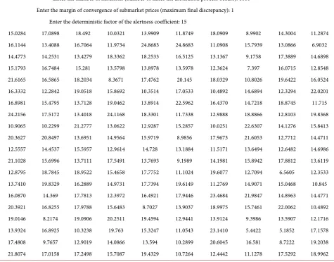
Each simulation involves running the program only once for a set of parameters entered by the user. The program performs several iterations until the reported convergence condition is reached. The first simulation was done for 10 submar-kets in which initial prices were drawn by the computer based on Equation (3.3). Prices are placed in increasing order and are associated with sub-markets from 1 to m. The user informs the number n of agents that will act in each submarket (total number of agents n m× ), the number N of iterations in the program loop (the number of times the arbitrage occurs), the convergence margin M of the prices of different submarkets (maximum permissible final discrepancy), the de-terministic factor τ of the alertness coefficient, the deterministic factor d of Equ-ation (11) used as a parameter of the price equEqu-ation. The values initially reported are m = 10, n = 20, N = 100, M = 1, τ= 5, d = 0.1. Flexibility coefficients k
j
σ
are generated by programs based on a uniform distribution function of 0 to 1 and used in estimating the total supply variation (demand, if negative) in each submarket. Therefore, initially in the face of Equation (3.11), the parameter bk is drawn for each k. Table 1 shows, for a simulation, the output on the Matlab screen with these coefficients for n m× agents, as well as the parameters bk for the price equation determined by the deterministic value d informed and by the draw in the uniform distribution. These values will remain the same throughout any simulation for a given d.Then, it estimates the Equation (3.4) of the research effort of each agent translated by a normal distribution function around the initial price of the market in question. The program through two loops going through all the sub-markets and all the agents makes such an estimate. In each case, the draw of a specific point is made throughout the distribution function that governs the price search effort. Table 2 shows the exit of the prices drawn, in the hundredth iteration, around each of the initial prices of the different submarkets. The sys-tem reveals, as a result of the draws in question, the submarkets discovered by each of the agents operating in the m submarkets. Such an estimate is made based on Equation (3.5) which translates into a specific programming sequence.
The system generates the
Z
k matrix of zeros and 1, which translates linked17From Equation (3.1), it follows that, at each iteration, k k
(
k k)
f i k i fp −p =b x −x and therefore
(
)
k k k k
f i k f i
p =p −b x −x .
or discovered markets by agents from all other submarkets. Next, the matrix with the price differences between the submarkets now connected and the sub-markets of origin is produced. The next step in the simulation is to estimate the supply variation (demand) in each submarket. This is done with agents starting at the same time from all the submarkets in question. Equation (3.12) is used to estimate the final price in the submarkets after each iteration. From one iteration to another, the system automatically proceeds in the simulation exercise up to the number of them informed. At the end of the hundredth iteration, Table 3 shows the Matlab output with the variation of the supply (demand) in each submarket, for this iteration, by line and by agents starting from different sub-markets, and the total variation of the supply in each submarket.18
Table 1. Determining factor of the price function (d), flexibility coefficients drawn ( k j
σ ), and parameters drawn for the price equ-ation (bk).
Command Window
Enter the coefficient of the price function (coefb): 0.1 Flexibility coefficients:
0.7335 0.3863 0.3565 0.3630 0.1203 0.2723 0.6235 0.7443 0.6065 0.4486 0.3050 0.4064 0.1628 0.4236 0.2208 0.8772 0.5033 0.3084 0.6005 0.1200 0.3115 0.2975 0.4059 0.1499 0.9641 0.9668 0.6292 0.9751 0.8981 0.1587 0.0064 0.1605 0.9644 0.7089 0.4309 0.9028 0.8656 0.0051 0.8080 0.4875 0.9661 0.3053 0.4073 0.8878 0.5027 0.7696 0.8460 0.2745 0.1200 0.4939 0.0721 0.8305 0.0418 0.2667 0.5176 0.4907 0.3461 0.7053 0.7204 0.1250 0.2444 0.3857 0.4326 0.4285 0.6502 0.5790 0.8241 0.1643 0.5385 0.1408 0.6067 0.1276 0.1450 0.1566 0.6992 0.3490 0.6325 0.4607 0.6848 0.5976 0.9593 0.1626 0.7057 0.9105 0.7786 0.8800 0.9464 0.6434 0.3790 0.4196 0.1420 0.4706 0.1593 0.9439 0.5305 0.4050 0.8367 0.5592 0.5325 0.6135 0.3343 0.5243 0.7518 0.8097 0.5875 0.9905 0.7250 0.2032 0.2839 0.3009 0.4355 0.5585 0.0752 0.7222 0.5500 0.5676 0.3900 0.0331 0.9466 0.2268 0.9307 0.7296 0.8149 0.5299 0.5598 0.1570 0.0372 0.2597 0.5205 0.8687 0.8848 0.1778 0.7064 0.2766 0.1126 0.1399 0.7117 0.7188 0.3995 0.5547 0.5314 0.2730 0.9648 0.6599 0.4132 0.3261 0.0204 0.0523 0.9130 0.6125 0.2944 0.1950 0.1405 0.0222 0.1998 0.2253 0.4425 0.4793 0.8154 0.7119 0.7734 0.5302 0.2461 0.7559 0.5617 0.5161 0.8715 0.6854 0.5013 0.5301 0.6341 0.7872 0.3510 0.6971 0.8128 0.8059 0.9876 0.9042 0.1782 0.3320 0.2175 0.8586 0.1167 0.3565 0.6019 0.5831 0.0129 0.2656 0.2500 0.9382 0.3574 0.3067 0.2025 0.4550 0.9782 0.8248 0.7020 0.9786 0.3413 0.6306
Parameters of the price equation. b=
0.0967 0.0989 0.0415 0.0700 0.0352 0.0192 0.0619 0.0401 0.0775 0.0954
Source: Result of the simulation in Matlab, given the program and parameters provided by the user.
18By rows, we interpret only movements of the nth agents of each column. Where n represents the location of the line counting vertically from top to bottom. The hundredth iteration corresponds to the maximum number of turns reported in the programming loop.
Table 2. Prices drawn around respective initial prices. 100th iteration.
Prices drawn around each starting price point
Observation: columns = submarkets//lines = agents
8.9562 14.2309 10.9892 18.0557 43.3676 43.4348 53.5571 55.5907 76.1003 94.4248 20.0764 13.4117 16.8516 8.5792 47.9399 51.9469 48.6588 58.2611 82.6683 97.9329 15.9174 20.4695 10.1907 12.9504 54.6789 48.6118 49.6280 57.4859 80.2394 99.2911 20.2459 23.4496 16.9068 21.5803 48.6266 56.9500 42.7496 48.4849 64.2941 98.4178 21.4155 14.3010 9.8855 17.1028 45.6796 55.7117 46.7486 53.1716 77.4461 92.8577 21.8430 14.9120 16.1868 18.7540 51.3319 49.1490 48.3029 49.3155 71.4437 92.6695 21.8542 11.7773 18.8712 19.0443 49.7780 38.1676 44.0721 48.7828 68.0812 94.1849 11.5401 11.5408 9.8954 13.6408 56.8756 48.4937 50.9833 49.1372 64.2041 99.0884 24.6165 18.6104 8.7036 18.5248 44.7098 47.2630 56.5068 37.7310 85.4037 100.2895 18.5987 19.1233 10.7648 12.7935 43.1336 53.8849 52.5609 45.3918 72.0079 94.2681 28.6056 18.9915 18.1280 6.2158 47.4831 52.1795 46.1789 55.7840 71.7928 89.9104 10.7304 6.3721 12.3575 11.6236 43.4721 49.5738 48.2879 44.4095 74.1891 98.8453 22.0650 17.6688 14.1423 21.3358 44.9731 46.2245 51.4606 56.7083 72.2050 99.7300 21.3438 10.6595 19.8467 10.6366 47.8336 46.4431 56.5116 46.1849 71.8851 98.4841 16.0873 18.3277 10.8991 20.8258 42.5873 48.0865 56.6684 53.1978 72.1600 101.1206 17.3959 11.6630 22.0149 11.1004 46.1730 47.8540 42.5840 44.7233 72.4370 100.6406 12.0568 16.1859 18.7431 17.4003 41.6170 40.5500 47.6658 40.4568 78.2790 96.0873 20.4163 10.4177 18.3128 13.7214 55.9853 49.2077 53.3346 47.1258 67.9835 91.7779 26.5303 11.3198 18.5146 13.1487 54.9889 53.3424 52.7799 44.8291 78.3463 96.5727 18.8382 14.3279 10.9800 15.0172 41.7529 51.6825 45.1925 35.7020 63.6955 97.2520
Source: Result of the simulation in Matlab. Prices generated in the hundredth iteration.
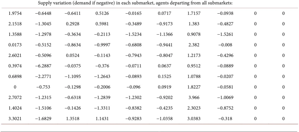
Table 3. Results at the end of the 100th iteration. Total net supply in linked markets for each agent in different submarkets. Total net supply for all agents in each submarket. Vectors of initial prices and at the end of the hundredth iteration.
Supply variation (demand if negative) in each submarket, agents departing from all submarkets:
1.9754 −0.6448 −0.6411 0.5126 −0.0165 0.0717 1.7157 −0.0938 0 0 2.1518 −1.3045 0.2928 0.5981 −0.3489 −0.9173 1.383 −0.4827 0 0 1.3588 −1.2978 −0.3634 −0.2113 −1.5234 −1.1366 0.9078 −1.5261 0 0 0.0173 −0.5152 −0.8634 −0.9997 −0.6808 −0.9441 2.382 −0.008 0 0 2.6021 −0.5096 0.0524 −0.1143 −0.7943 −0.8047 1.2173 −0.4296 0 0 0.3974 −6.2887 −0.0375 −0.376 −0.0711 0.0637 0.9512 −0.0889 0 0 0.6898 −2.2771 −1.1095 −1.2643 −0.0893 0.1525 1.0788 −0.0207 0 0 0 −0.753 −0.1298 −0.2006 −0.096 0.0919 1.8227 −0.0581 0 0 2.7072 −1.2315 −0.6318 −1.2839 −1.2302 −0.9202 3.966 −1.0069 0 0 1.4024 −1.5106 −0.1426 −1.3311 −0.8382 −0.4235 2.3023 −0.8752 0 0 3.3021 −1.6829 1.3518 1.1431 −0.9283 −1.0358 3.0383 −0.318 0 0
[image:14.595.57.540.525.738.2]Continued
1.229 −0.8605 0.1351 1.0197 −0.8691 −0.5936 1.0732 −0.0518 0 0 2.5066 −1.218 0.1049 −0.0682 −0.8844 −0.1642 0.1557 −0.4064 0 0 8.7401 −0.5708 1.2701 0.3905 −0.1779 −0.1463 2.9824 −1.1249 0 0 1.4995 −1.6115 −0.8638 −0.9306 −0.6528 −0.341 0.0853 −0.0818 0 0 0 −0.3004 0.2527 0.0314 −0.0274 0.0593 1.8545 −0.0604 0 0 2.0831 −0.8851 0.4425 1.0672 −0.8875 −0.5397 3.6523 −1.0727 0 0 3.4972 −2.5267 0.0452 −0.0897 −1.2843 −0.8427 2.714 −1.415 0 0 1.1994 −2.7561 −0.2993 −1.052 −0.951 −0.6098 0.0541 −0.4157 0 0 2.5678 −0.4725 −0.1813 0.6424 −1.5457 −0.8625 1.9292 −1.5315 0 0
Total variation of supply (demand if negative) in each submarket. All agents:
39.927 −29.2172 −0.0336 −2.5169 −13.8973 −9.8428 35.2658 −11.702 0 0 *** Initial and final price vector in iteration:
100
Vector of initial prices:
0.1701 6.2000 16.6108 22.1575 35.1243 46.7762 47.0506 57.1393 71.8806 96.7954 Vector of final prices:
12.1464 14.5361 13.3160 13.3619 47.2809 47.1149 46.0506 47.2394 70.5470 96.7954
Source: Result of the simulation in Matlab.
It also shows, at the end of it, the final prices, which are compared to the pric-es initially drawn. In this case, it is the hundredth iteration, because the loop of the program that commands the process of iterative approximation to the mar-gin of convergence reported by the user was executed a hundred times, the N
number informed. For different N informed, the number of iterations would have been naturally different.
At the end, a final price vector pf is given in the table above. It should be
noted that, in this case, there was no convergence between prices. However, in-stead of stating that the convergence process is not possible, the model for dif-ferent calibration parameters is tested. If it keeps the same parameters of the previous simulation, it now evaluates the simulation model for different alert-ness coefficients τ, in the values of 10, 15, 20 and 25. In each case, the same coef-ficients of flexibility k
j
σ
and the same parameters of the price equation is maintained, both in Table 1. The initial price vector is also the same for each simulation involving a specific τ. In all these simulations, it is first necessary to examine the degree of linkage that is obtained between the 10 submarkets in question. To do so, a procedure is developed that generates Table 4 where the number indicates quantities of agents arbitrating the respective submarkets for agents located in the same line (of the 20 lines generated in each submarket), in-cluding the agent of origin, which was already in the submarket. Any number greater than 1 indicates, therefore, connection between submarkets.Table 4. Results of linking submarkets to the end of the 100th iteration. Linked markets and “degree of connection”. Command Window
Degree of market linkage: Markets directly linked for agents departing from the submarket:
By agent group: 8
2 2 3 3 3 3 3 3 1 1 See the entries in which appears the numeral 1:
3 3 3 3 4 4 3 4 1 1 0 0 0 0 1 1 0 1 0 0
2 2 4 4 4 3 2 4 1 1 0 0 0 0 1 1 1 1 0 0
2 3 4 4 4 4 3 4 1 1 0 0 0 0 1 0 0 1 0 0
2 2 2 2 4 4 2 4 1 1 0 0 0 0 1 1 0 1 0 0
3 4 4 4 3 2 3 3 1 1 0 0 0 0 1 1 1 1 0 0
2 3 3 3 3 3 2 3 1 1 0 0 0 0 1 1 1 1 0 0
1 3 4 3 3 3 3 3 1 1 0 0 0 0 1 1 0 1 0 0
2 4 4 4 4 4 4 4 1 1 0 0 0 0 1 1 1 1 0 0
4 3 4 4 4 4 3 4 1 1 0 0 0 0 1 1 1 1 0 0
4 3 3 3 4 4 4 4 1 1 0 0 0 0 1 1 0 1 0 0
2 2 3 3 4 4 3 4 1 1 0 0 0 0 1 1 1 1 0 0
2 2 2 2 4 4 4 4 1 1 0 0 0 0 1 1 0 1 0 0
4 3 3 3 4 4 4 4 1 1 0 0 0 0 1 1 1 1 0 0
2 3 4 4 4 4 4 4 1 1 0 0 0 0 1 1 1 1 0 0
1 2 3 3 3 3 4 3 1 1 0 0 0 0 1 1 1 1 0 0
2 2 3 3 4 4 4 4 1 1 0 0 0 0 1 1 1 1 0 0
3 3 2 2 4 4 3 4 1 1 0 0 0 0 1 1 1 1 0 0
3 3 3 3 4 4 4 4 1 1 0 0 0 0 1 1 1 1 0 0
3 2 4 3 4 4 3 4 1 1 0 0 0 0 1 1 1 1 0 0
For all agents: 0 0 0 0 1 1 1 1 0 0
49 54 65 63 75 73 65 75 20 20 Markets directly linked: 4
Source: Result of the simulation in Matlab. Hundredth iteration.
These markets are not always directly linked. Market with such link can be seen in the right part of the table for agents departing from submarket 8, which discriminates the markets that he can exploit from that point (which receive the number 1). For agents starting from the submarket in question, there are at most 4 markets directly linked. Other results for linking are found for agents starting from other submarkets. For the given simulation, in the hundredth iteration, the maximum connection that was obtained was 4 markets directly linked to agents starting from the 1 to 8 markets. The program also accuses when no market is linked to another (in the case of agents that depart from markets 9 and 10).
The table to the left of Table 4 is obtained by summing the unit inputs of agents, in the same lines in the table, starting from a certain submarket. The ag-gregate number should be interpreted as the degree of connection of the sub-markets, it indicates the number of agents located in the line of the table, which acts in the linking of a market with some of the others. The last line of the table on the left should be interpreted as the overall degree of linking of the submarket
in question to some of the others, considering all the agents that have in the submarket their base.
Note that these tables only relate to the connections obtained in the last itera-tion, which starts from the price vector established in the penultimate round, since prices are possibly other for each iteration and, therefore, the submarket links. Markets are linked in the round in question, then switched off, and poten-tially tied again in the next iteration. The connection is not definitive, since the prices practiced in the submarkets change with each iteration and the agents de-part again to the process of search of advantageous prices and discovery of op-portunities of arbitration every round.
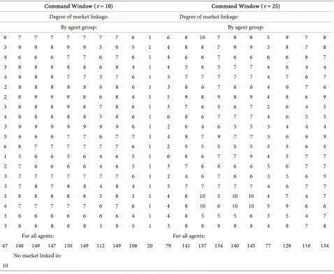
[image:17.595.61.540.323.715.2]Keeping the same basic parameters, then new simulations were done for dif-ferent coefficients of alertness τ. We work with the values of 10, 15, 20 and 25. Table 5 shows the degree of linkage of the submarkets to the end of the hun-dredth iteration for the first and last value. Simulations were also generated for intermediate values.
Table 5. Degree of connection of the submarkets to the end of the 100th iteration. Two coefficients of alertness τ. (d = 0.1).
Command Window (τ = 10) Command Window (τ = 25)
Degree of market linkage: Degree of market linkage:
By agent group: By agent group:
6 7 7 7 7 7 7 7 6 1 6 8 10 7 8 8 5 9 7 8
3 9 9 8 9 9 5 9 5 1 4 8 8 7 9 9 3 8 7 8
4 6 6 6 7 7 6 7 6 1 4 6 6 7 6 6 6 6 8 7
3 8 8 8 8 8 6 8 4 1 4 5 6 5 7 7 4 6 4 4
4 8 8 8 7 7 5 7 6 1 5 7 7 7 7 7 4 7 6 7
2 8 8 8 8 8 6 8 6 1 3 6 6 7 6 6 4 6 7 6
2 8 9 9 9 8 6 8 4 1 5 9 8 9 8 9 4 8 6 9
3 8 8 8 9 8 7 8 6 1 3 7 6 5 6 7 2 6 4 5
4 8 8 8 8 8 5 8 6 1 6 8 6 7 7 7 4 6 5 5
3 9 9 9 9 9 9 9 6 1 2 6 4 6 5 5 3 4 4 4
5 6 6 6 7 7 6 7 7 1 4 8 7 9 7 7 3 6 6 9
6 8 7 7 7 7 7 7 6 1 2 5 5 5 5 5 3 5 6 5
1 5 6 6 5 6 4 6 5 1 6 8 6 7 7 9 4 5 7 7
2 7 6 6 6 6 4 6 5 1 3 7 6 8 6 6 5 6 7 7
3 7 7 7 7 7 7 7 6 1 2 4 6 7 6 6 3 5 6 5
3 7 8 7 8 8 4 8 4 1 5 7 7 7 7 7 4 6 7 7
3 8 8 8 8 8 3 8 3 1 4 8 10 5 10 10 4 7 4 7
4 7 7 7 7 7 6 7 6 1 4 8 10 6 10 10 5 9 6 6
3 6 6 6 6 6 6 6 4 1 4 8 5 5 5 6 3 5 4 7
3 8 8 8 8 8 3 8 5 1 3 8 8 8 8 8 4 8 7 8
For all agents: For all agents:
67 148 149 147 150 149 112 149 106 20 79 141 137 134 140 145 77 128 118 134 No market linked in:
10
Source: Result of the simulation in Matlab. Hundredth iteration.
Graph 2 shows the trajectory of prices between submarkets, with the succes-sive discovery of new markets and the arbitrage process, for the different coeffi-cients of alertness applied to the problem under analysis, given the values adopted in the other parameters. In all simulations, the initial prices are the same, by construction, and the final submarket price vector is shown, in the dif-ferent contexts, in 10 steps equally spaced up to the hundredth iteration.
It should be noted that, even increasing the deterministic coefficient of alert-ness, homogeneous prices were not obtained in all submarkets considered.
Graph 2. Evolution of submarket prices in 10 steps. Final prices in the 100th iteration. Same initial prices in different simulations. Different coefficients of alertness τ (d = 0.1). (a) τ = 5; (b) τ = 10; (c) τ = 15; (d) τ = 20; (d) 25. Source: Result of the simulation in Matlab, given the program and parameters provided by the user. Output in EXCEL. Hundredth iteration.
Differently from the theoretical statements of Littlechild and Owen [1], in the simulation exercise there was no price convergence, only that the prices of the different submarkets tend to oscillate in an intermediate price range between the extreme values. Even increasing the value of the alertness, the system does not converge. However, the results of the numerical simulation may be other, and the system behaves dynamically in another way, when the values assigned to the basic parameters change in the exercise. Indeed, by making the deterministic product d of Equation (3.11), which regulates the price formation in Equation (3.12), assume a value less than 0.1, it is observed that the system has a more sta-ble behavior, with the dynamic convergence of submarket prices to the same uniform value. In fact, a new set of graphs with the evolution of submarket pric-es can be obtained by making, for example, the coefficient d assuming, by cali-bration, the value of 0.01.
Graph 3 remakes price trajectories in the simulations and presents its evolu-tion in a similar way to that of the previous figure, considering now the new value assigned to the parameter of the price equation. The new figure shows the evolution of the system to the alertness τ assuming values of 5, 10, 15 and 20.
Thus, in this case, uniform prices in the different submarkets are already formed with an alertness coefficient equal to 20. So the convergence process de-pends on the level of alertness of the entrepreneurs, but also on the parameters of the price equation, of how the new prices respond to the excesses of net supply that are being formed in the submarkets per action of the arbitration process. Table 6 shows the degree of binding of the submarkets to
τ
=10 and25 for the purpose of comparing the behavior of the system with the new deter-ministic factor d of the price equation in 0.01, in relation to the linking results for d= 0.1 of the previous exercise.
It should be noted that with the price equation parameter only 10% of the previous level, not only the convergence of submarket prices in the simulations is guaranteed, but also a considerably greater degree of linkage between the markets. By comparing Table 5 and Table 6, the highest values of connections cues in the case with a lower d and
τ
=25 are apparent. More precisely, in thiscase the mean degree of link increases from 123.1 to 194.5. Interestingly, the same does not occur for τ = 10.
Similar simulations were done for even lower values of d. Note that with the deterministic parameter of the price equation very low, say d = 0.001, there is no price convergence for an alertness of 20. In order to evaluate the effect of the factor d on convergence, an exercise is done with a big number of iterations (up to one thousand), and it evaluates the number of iterations that are necessary to allow the convergence of submarket prices to occur in terms of the values as-sumed by the parameter in question. It assumes in all the exercises that the alertness is 20. Graph 4 shows the relationship between the parameter d of the price equation and the number of iterations for the convergence of submarket prices to occur. The economic interpretation of this graph is that when the
coefficient d falls in a range between 0.008 and 0.018, specific to the parameters informed and the simulation exercise in question, convergence occurs in a smaller number of iterations, that is, it is performed more efficiently.
Note that, for
τ
=20, there is no price convergence between submarkets, forup to 1.000 iterations, for d = 0.001, and that the convergence occurs rapidly for
[image:20.595.59.536.326.716.2]d = 0.01, according to previous simulations (Graph 4). The range of d between 0.0075 and 0.02 is quite favorable for convergence at homogeneous prices in the simulations, however, such convergence does not occur easily (and may never occur) when d assumes values outside this range. Then the dynamic behavior of the prices in the simulations depends on the calibration of the model. It depends fundamentally on the parameter of the price equation and depends naturally on the alertness τ. Regarding the alertness, it sees in Table 6 how crucial to gence it is. In fact, a greater degree of alertness facilitates the process of conver-gence. Next, it is investigated by means of new simulations, to what extent a greater degree of entrepreneurial alertness facilitates the convergence of prices.
Table 6. Degree of connection of the submarkets to the end of the 100th iteration. Two coefficients of alertness τ (d = 0.01).
Command Window (τ = 10) Command Window (τ = 25)
By agent group: Degree of market linkage:
4 4 4 4 5 5 5 5 5 1 By agent group:
4 4 4 4 4 4 5 4 4 1 10 10 10 10 10 10 10 10 10 10 5 4 4 4 5 5 5 5 5 1 10 10 10 10 10 10 10 10 10 10 4 4 4 4 5 5 5 5 5 1 10 10 10 10 10 10 10 10 10 10 4 3 3 3 5 5 5 5 5 1 10 10 10 10 9 10 10 10 10 10 3 4 3 3 5 5 4 5 5 1 10 10 10 10 10 10 10 10 10 10 4 4 4 4 5 5 5 5 5 1 10 10 10 10 9 10 10 10 10 10
3 3 4 3 5 5 5 5 5 1 10 9 9 9 9 9 9 9 9 9
4 4 4 4 5 5 5 5 5 1 10 10 10 10 10 10 10 10 10 10 4 4 4 4 5 5 5 5 5 1 10 10 10 10 9 10 10 10 10 10 3 3 3 4 5 5 5 5 5 1 10 10 10 10 10 10 10 10 10 10
5 4 4 4 5 5 5 5 5 1 9 9 9 9 10 9 9 9 9 9
4 4 4 4 4 5 4 5 5 1 9 9 9 9 9 10 9 9 9 9
4 4 4 4 5 5 5 5 5 1 9 9 9 9 10 9 9 9 9 9
4 4 4 4 5 5 5 5 5 1 9 9 9 10 9 9 9 9 9 9
4 4 4 4 5 5 5 5 5 1 9 10 9 10 9 10 9 9 10 9
4 4 4 4 5 5 4 5 5 1 10 10 10 10 10 10 10 10 10 10 4 4 4 4 5 5 5 5 5 1 10 10 10 10 9 10 10 10 10 10 4 4 4 4 5 5 5 5 5 1 10 10 10 10 10 10 10 10 10 10 4 4 4 4 4 5 5 5 5 1 10 10 10 10 10 10 10 10 10 10 10 10 10 10 10 10 10 10 10 10
For all agents: For all agents:
79 77 77 77 97 99 97 99 99 20 195 195 194 196 192 196 194 194 195 194
Source: Result of the simulation in Matlab. Hundredth iteration.
Graph 3. Evolution of submarket prices in 10 stages. Final prices in the 100th iteration. Same initial prices in different simulations. Different coefficients of alertness degree τ (d = 0.01). (a) τ = 5; (b) τ = 10; (c) τ = 15; (d) τ = 20. Source: Result of the simulation in Matlab, given the program and parameters provided by the user. Output in EXCEL. Hundredth iteration.
Graph 4. Relationship between the parameter d of the submarkets price equation and the number of iterations of the program so that price convergence occurs in the stipulated margin of 1. τ = 20. Decimal separations with commas. Source: Result of the simulation in Matlab, given the program and parameters provided by the user. Output in EXCEL.
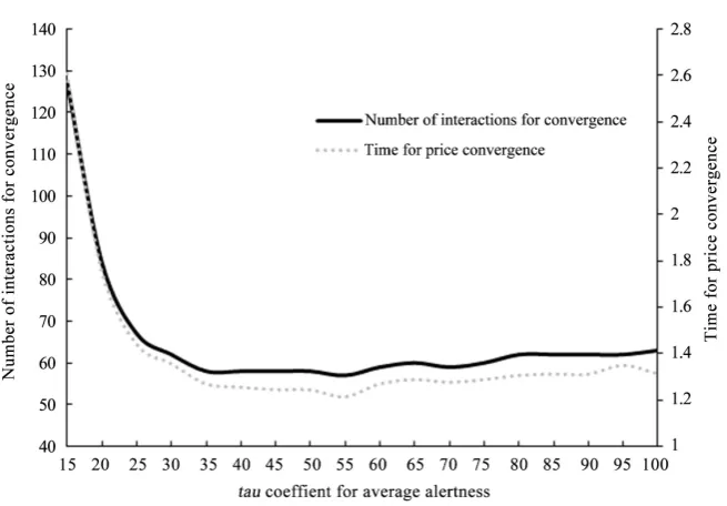
Graph 5 shows the relationship between τ and the number of iterations re-quired for the convergence of submarket prices. In all simulations d = 0.01was used. As seen previously, in the simulations, for the alertness below 20, there is no price convergence in the submarkets. The convergence velocity seems in-creasing for τ increasing up to 50, with some oscillation. However, it is noted that a higher value of the alertness, above this level, does not have a well-defined relation with the speed of price convergence. In fact, by examining the behavior of the curve in Graph 5, it is clear that, from a certain level, a greater degree of entrepreneurial alertness has no systematic effect on convergence. For
50≤ ≤
τ
200, an oscillatory pattern is observed in the relation between τ andconvergence velocity. In the next step of the paper, it is analyzed the relationship between the alertness coefficient and processing time until the convergence of prices in the submarkets is reached.
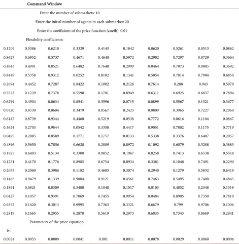
Therefore, it is still worth to examine the dynamic behavior of the numerical simulation model taking into account the processing time of the computer.19 For this exercise, all “pause” commands of the program in Matlab have been deleted. Simulations are performed for up to a thousand iterations, at the end of which the number of iterations for price convergence and the associated time in seconds are computed. For the exercise in question, a new vector of initial prices in the submarkets is drawn. Table 7 shows the output screen of the first simula-tion again indicating the case of 10 submarkets, 20 agents in each. The new drawn transfer coefficients are shown. The simulation is done initially for de-terministic coefficient of alertness of 15. New simulations, with the same basic parameters of this, will be made for different values of τ, from 20 to 100, varying 5.
Graph 5. Relation between the alert level (τ) and the number of iterations of the program in order for price convergence to occur at the stipulated margin of 1 (d = 0.01). Source: Result of the simulation in Matlab, given the program and parameters provided by the user. Output in EXCEL.
19Processing time should be seen as a measure of the efficiency of the price convergence process.
Table 7. Number of submarkets (m), number of agents in each (n), deterministic factor of the price function (d), drawn flexibility coefficients ( k
j
σ ) and drawn parameters for the price equation (bk).
Command Window
Enter the number of submarkets: 10
Enter the initial number of agents in each submarket: 20 Enter the coefficient of the price function (coefb): 0.01 Flexibility coefficients:
0.1209 0.5386 0.6210 0.3329 0.4145 0.1842 0.0620 0.5261 0.0513 0.0862 0.8627 0.6952 0.5737 0.4671 0.4648 0.5972 0.2982 0.7297 0.0729 0.3664 0.4843 0.4991 0.0521 0.6482 0.7640 0.2999 0.0464 0.7073 0.0885 0.3692 0.8449 0.5358 0.9312 0.0252 0.8182 0.1341 0.5054 0.7814 0.7984 0.6850 0.2094 0.4452 0.7287 0.8422 0.1002 0.2126 0.7614 0.288 0.943 0.5979 0.5523 0.1239 0.7378 0.5590 0.1781 0.8949 0.6311 0.6925 0.6837 0.7894 0.6299 0.4904 0.0634 0.8541 0.3596 0.0715 0.0899 0.5567 0.1321 0.3677 0.0320 0.8530 0.8604 0.3479 0.0567 0.2425 0.0809 0.3965 0.7227 0.2060 0.6147 0.8739 0.9344 0.4460 0.5219 0.0538 0.7772 0.0616 0.1104 0.0867 0.3624 0.2703 0.9844 0.0542 0.3358 0.4417 0.9051 0.7802 0.1175 0.7719 0.0495 0.2085 0.8589 0.1771 0.1757 0.0133 0.5338 0.3376 0.6407 0.2057 0.4896 0.5650 0.7856 0.6628 0.2089 0.8972 0.1092 0.6079 0.3288 0.3883 0.1925 0.6403 0.5134 0.3308 0.9052 0.1967 0.8258 0.7413 0.6538 0.5518 0.1231 0.4170 0.1776 0.8985 0.6754 0.0934 0.3381 0.1048 0.7491 0.2290 0.2055 0.2060 0.3986 0.1182 0.4685 0.3074 0.2940 0.1279 0.5832 0.6419 0.1465 0.9479 0.1339 0.9884 0.9121 0.4561 0.7463 0.5495 0.7400 0.4845 0.1891 0.0821 0.0309 0.5400 0.1040 0.1017 0.0103 0.4852 0.2348 0.1518 0.0427 0.1057 0.9391 0.7069 0.7455 0.9954 0.0484 0.8905 0.7350 0.7819 0.6352 0.1420 0.3013 0.9995 0.7363 0.3321 0.6679 0.799 0.9706 0.1006 0.2819 0.1665 0.2955 0.2878 0.5619 0.2973 0.6035 0.7343 0.8669 0.2941
Parameters of the price equation. b=
0.0024 0.0053 0.0009 0.0041 0.001 0.0011 0.0078 0.0029 0.0060 0.0096
Source: Result of the simulation in Matlab, given the program and parameters provided by the user.
This new vector of initial prices in the submarkets is pi = (10.9755; 18.7461; 26.6179; 43.2485; 43.2642; 65.5498; 69.4752; 75.8099; 79.7830; 93.3760) and the price vector at the end of the 127th interaction is pf= (47.9075; 48.0096; 47.3818; 48.0051; 48.1018; 48.8615; 48.0196; 47.9994; 48.0165; 48.0226) for the initial case with
τ
=15. The processing time was, in this case, 2.6051 seconds until theconvergence of the submarkets prices.
Graph 6 shows the relationship between the alertness (τ) and the convergence