1
Local Characteristics of and Exposure to Fine Particulate Matter (PM
2.5) in
1Four Indian Megacities
2
Ying Chen1*, Oliver Wild1, Luke Conibear2,Liang Ran3, Jianjun He4, Lina Wang5, Yu Wang6 3
1Lancaster Environment Centre, Lancaster University, Lancaster, LA1 4YQ, UK
4
2Institute for Climate and Atmospheric Science, School of Earth and Environment, University
5
of Leeds, UK
6
3Key Laboratory of Middle Atmosphere and Global Environment Observation, Institute of
7
Atmospheric Physics, Chinese Academy of Sciences, Beijing, 100029, China
8
4State Key Laboratory of Severe Weather & Key Laboratory of Atmospheric Chemistry of
9
CMA, Chinese Academy of Meteorological Sciences, Beijing, 100081, China
10
5Shanghai Key Laboratory of Atmospheric Particle Pollution and Prevention, Department of
11
Environmental Science and Engineering, Fudan University, Shanghai 200433, China
12
6Centre for Atmospheric Sciences, School of Earth and Environmental Sciences, University of
13
Manchester, Manchester, M13 9PL, UK
14
Correspondence to: Ying Chen (y.chen65@lancaster.ac.uk)
15 16 17
Highlights:
18
• PM2.5 increased by 75% during Diwali in Delhi, causing 20 extra daily mortality
19
• A weekend effect is found in Mumbai and Chennai but not in Delhi and Hyderabad
20
• Distinct differences in diurnal pattern of PM2.5 in different seasons and cities
2
Abstract:
22
Public health in India is gravely threatened by severe PM2.5 exposure. This study presents an
23
analysis of long-term PM2.5 exposure in four Indian megacities (Delhi, Chennai, Hyderabad
24
and Mumbai) based on in-situ observations during 2015-2018, and quantifies the health risks
25
of short-term exposure during Diwali Fest (usually lasting for ~5 days in October or November
26
and celebrating with lots of fireworks) in Delhi for the first time. The population-weighted
27
annual-mean PM2.5 across the four cities was 72 µg/m3, ~3.5 times the global level of 20 µg/m3
28
and 1.8 times the annual criterion defined in the Indian National Ambient Air Quality Standards
29
(NAAQS). Delhi suffers the worst air quality among the four cities, with citizens exposed to
30
‘severely polluted’ air for 10% of the time and to unhealthy conditions for 70% of the time.
31
Across the four cities, long-term PM2.5 exposure caused about 28,000 (95% confidence interval:
32
17,200–39,400) premature mortality and 670,000 (428,900–935,200) years of life lost each
33
year. During Diwali Fest in Delhi, average PM2.5 increased by ~75% and hourly concentrations
34
reached 1676 µg/m3. These high pollutant levels led to an additional 20 (13–25) daily
35
premature mortality in Delhi, an increase of 56% compared to the average over
October-36
November. Distinct seasonal and diurnal variations in PM2.5 were found in all cities. PM2.5
37
mass concentrations peak during the morning rush hour in all cities. This indicates local traffic
38
could be an important source of PM2.5, the control of which would be essential to improve air
39
quality. We report an interesting seasonal variation in the diurnal pattern of PM2.5
40
concentrations, which suggests a 1-2 hours shift in the morning rush hour from 8 a.m. in
pre-41
monsoon/summer to 9-10 a.m. in winter. The difference between PM2.5 concentrations on
42
weekdays and weekend, namely weekend effect, is negligible in Delhi and Hyderabad, but
43
noticeable in Mumbai and Chennai where ~10% higher PM2.5 concentrations were observed in
44
morning rush hour on weekdays. These local characteristics provide essential information for
3
air quality modelling studies and are critical for tailoring the design of effective mitigation
46
strategies for each city.
47
Keywords: PM2.5; Health effect; Diwali festival effect; Weekend effect; Long-term;
Short-48
term
49 50
1. Introduction
51
Exposure to fine particulate matter (particles with an aerodynamic diameter less than 2.5
52
µm, PM2.5) can pose a major threat to human health (Chowdhury and Dey, 2016; Gao et al.,
53
2018a; Gao et al., 2017; Huang et al., 2018; Pope et al., 2009; Wang et al., 2017). As a rapidly
54
developing country with an expanding population, India is suffering severe PM2.5 pollution,
55
with nine cities among the top ten most polluted cities in the world as reported by the World
56
Health Organization (WHO, 2016). Exposure to high levels of PM2.5 causes ~1 million
57
premature mortality per year across India (Conibear et al., 2018a). In order to tackle this PM2.5
58
pollution, the Central Pollution Control Board (CPCB) of India set revised National Ambient
59
Air Quality Standards (NAAQS) in 2009 that included PM2.5 regulations (CPCB, 2009). Some
60
mitigation policies have been implemented in major Indian cities(Chowdhury et al., 2017;
61
Sharma and Dixit, 2016), but limited improvement in air quality (~10% reduction in PM2.5) has
62
been seen (Chowdhury et al., 2017). PM2.5 pollution is expected to further deteriorate in the
63
coming decades (Chowdhury et al., 2018; Conibear et al., 2018b), due to rapid ongoing
64
urbanization. This surface pollution over India also has important global implications through
65
effective transport by the Asian summer monsoon to the upper troposphere and lower
66
stratosphere, where pollutants can be re-distributed on a global scale and thus affect global
67
climate forcing and air quality (Lelieveld et al., 2018; Liu et al., 2015; Yu et al., 2017).
4
Previous studies estimated health risks in India of exposure to PM2.5 based on model
69
analysis or satellite retrieves and mainly focused on long-term exposure (e.g., Chowdhury and
70
Dey, 2016; Conibear et al., 2018a, b; Gao et al., 2018b; Lelieveld et al., 2015; van Donkelaar
71
et al., 2015). In addition, intensive emissions and unfavourable meteorological condition for
72
dispersion can significantly increase PM2.5 and lead to hazardous short-term exposure with high
73
health risks (Atkinson et al., 2014; Héroux et al., 2015). In-situ observations at high temporal
74
resolution are valuable for more firmly grounded estimates of health risks. Furthermore,
75
characterizing the seasonal and diurnal variations of urban PM2.5 concentrations and their
76
relationships to meteorology is the key to understanding the drivers of air pollution and
77
devising effective mitigation strategies in Indian megacities (Schnell et al., 2018). Long-term
78
in-situ monitoring studies are critical for a better understanding of these factors. However, only
79
a few studies providing long-term observations of PM2.5 have been undertaken, and most of
80
these have focused on Delhi only (Sahu and Kota, 2017; Sharma et al., 2018). Information on
81
local characteristics such as the diurnal variation in pollutant emissions is also critical for
82
modelling studies. This information is scarce in India and models typically use a constant
83
diurnal profile of emissions (e.g., Mohan and Gupta, 2018) or standard profiles from American
84
or European cities to represent conditions in India (e.g., Marrapu et al., 2014). Long-term
85
observations of the diurnal variation of pollutants would provide essential information for
86
improving model performance.
87
This study presents a comprehensive summary of the seasonal and diurnal variation of
88
urban PM2.5 in four Indian megacities (Delhi, Chennai, Hyderabad and Mumbai), based on
89
ground observations from 2015 to 2018. This analysis reveals the observation-based patterns
90
of human activity and local temporal characteristics of emissions in each city, and hence
91
provides valuable input for modelling studies. In addition, for the first time, we report the
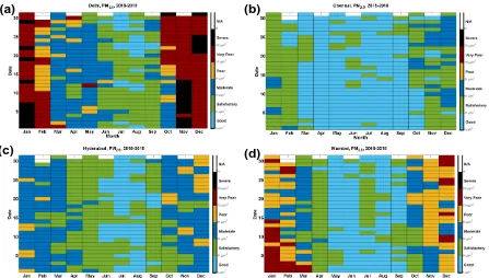
92
influences of weekend effect on the diurnal variations and quantify the health risks of
5
term exposure during Diwali Fest. Finally, the cumulative exposure of urban residents to PM2.5
94
and the corresponding health burdens are estimated for each city. The results of this study are
95
valuable for the designation and implementation of mitigation policies on a city level aimed at
96
improving air quality to meet the Indian NAAQS standards.
97 98
2. Materials and Methods
99
2.1 Data
100
Datasets of pollutants measured between 1 March 2015 and 31 December 2018 are
101
analysed in this study. An overview of the data is given in Table S1. Hourly PM2.5 observations
102
in Delhi, Chennai, Mumbai and Hyderabad (Fig. S1) are rountinely made at U.S. Embassy and
103
consulates using a beta attenuation monitor (San Martini et al., 2015). These records are
104
available from the AirNow website (https://www.airnow.gov/). The instruments are maintained
105
and calibrated following the regulations of the U.S. Environmental Protection Agency (EPA,
106
2009, 2015). PM2.5 observations from the U.S. Embassy are widely used in previous studies in
107
India (Wang and Chen, 2019) and China (Lv et al., 2017; Lv et al., 2015; San Martini et al.,
108
2015), and have been shown to be of good quality and in good agreement with other
109
observations (Jiang et al., 2015; Mukherjee and Toohey, 2016).
110
We use hourly meteorological observations at the airport in each city (VIDP-Delhi,
111
VOMM-Chennai, VABB-Mumbar and VOHY-Hyderabad). The flat topography surrounding
112
these airports suggests that the observations are broadly representative of the dominant
113
meteorological conditions in these cities. Historical records are archived by the National
114
Oceanic and Atmospheric Administration, and are available from the National Climatic Data
115
Center (https://www.ncdc.noaa.gov/data-access/). The height of the planetary boundary
116
layer (PBL) is obtained from the European Centre for Medium-Range Weather Forecasts
6
(ECMWF) ERA-interim reanalysis at a 3-hour interval and 0.125° × 0.125° spatial resolution
118
(https://www.ecmwf.int/).
119
2.2 Method
120
We estimate the long-term health impacts from exposure to ambient PM2.5 concentrations,
121
as these account for the majority of the health effects through capturing both acute and chronic
122
responses. Following our previous works (Conibear et al., 2018a, b), we use integrated
123
exposure-response (IER) functions (Burnett Richard et al., 2014), updated for the Global
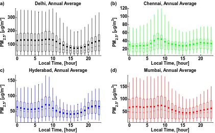
124
Burden of Disease GBD2016 (GBD, 2016) to estimate the relative risk (RR) of premature
125
mortality due to exposure to PM2.5 concentrations. There are IER functions with age-specific
126
modifiers for chronic obstructive pulmonary disease (COPD), lower respiratory infection (LRI),
127
ischaemic heart disease (IHD), cerebrovascular disease (CEV), and lung cancer (LC). We use
128
the parameter distributions from the GBD2016 for 1,000 simulations to derive the mean IER
129
with 95% uncertainty intervals. The IER functions have uniform theoretical minimum risk
130
exposure levels for PM2.5 between 2.4–5.9 µg/m3.
131
We use multi-year average annual-mean PM2.5 concentrations from measurements made
132
at U.S. diplomatic missions in Delhi (110 µg/m3), Chennai (33 µg/m3), Hyderabad (56 µg/m3),
133
and Mumbai (60 µg/m3). Baseline mortality data are taken from the GBD2016 for India (GBD,
134
2018). Population size was taken from the lastest Indian Census data for 2011. Population age
135
composition was taken from the GBD2016 population estimates for 2015 for India (GBD,
136
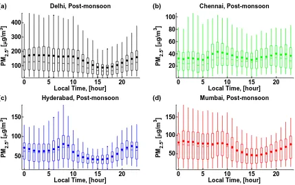
2017a).
137
Annual premature mortality (M) for each age and disease were estimated as a function of
138
population (P), baseline mortality rates (I), and the attributable fraction (AF) for a specific
139
relative risk (RR) (Equation 1). The disease burden from LRI, IHD, CEV, COPD, and LC was
140
estimated between 0 and 95 years upwards in 5 year groupings.
141
7
1
, RR
M P I AF AF
RR −
= = (1)
143
Annual years of life lost (YLL) for each age and disease were estimated as a function of
144
premature mortality and age-specific life expectancy (LE) from the standard reference life table
145
from the GBD2016 (Equation 2) (GBD, 2017b).
146
LE
M
YLL
=
(2)147 148
We estimate the short-term health impacts during Diwali Fest in Delhi from exposure to
149
ambient PM2.5 concentrations as all-cause premature mortality. The short-term health impacts
150
are accounted for within the long-term health impacts, and are used to indicate the variation in
151
the daily burden from acute responses (Héroux et al., 2015). We use the summary risk estimates
152
(γ) from Atkinson et al. (2014) of 1.04% (0.52–1.56) per 10 µg/m3 change in daily mean PM 2.5
153
concentrations (Cd), with respect to a reference PM2.5 concentration (Cr) of 0 µg/m3. We assume
154
no upper concentration cutoff. India-specific risk functions for ambient PM2.5 exposure do not
155
currently exist, however, the use of the summary risk estimate of 1.04% is conservative when
156
compared with the summary risk estimate of 1.2% from Levy et al. (2012) and 1.23% from
157
WHO (2013). Baseline mortality data are taken from the GBD2016 for India for all ages for
158
both genders combined (GBD, 2018). We convert these annual rates to daily rates (Id) by
159
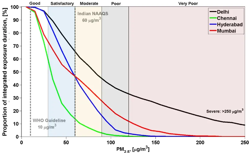
dividing by 365.25, consistent with previous work due to the lack of daily data (West et al.,
160
2007). We use first-three-day of Diwali Fest (320 µg/m3) and October-November two-month
161
(183 µg/m3) averaged daily-mean PM2.5 concentrations during 2015-2018 from the U.S.
162
Embassy measurements for Delhi.
163
8
d d d d
RR RR I P
M = −1 (4)
165
We use a linear exposure-response function with no cap on daily relative risk (RRd),
166
similar to a previous work (van Donkelaar et al., 2011), estimating daily relative risks following
167
Equation 3. Daily premature mortality (Md) is then estimated using Equation 4.
168
Using a logarithmic exposure-response function as in previous work (Crippa et al., 2016),
169
our estimates of short-term premature mortality are about 10% larger than with a linear
170
exposure-response function. To be conservative, we use the linear exposure-response function
171
in this study.
172 173
3. Results
174
3.1 Overview of PM2.5 in Four Megacities
175
The locations of Delhi, Chennai, Hyderabad and Mumbai are shown in Fig. 1, together
176
with annual mean surface concentrations of PM2.5 of anthropogenic origin over India in 2015
177
(van Donkelaar et al., 2015; van Donkelaar et al., 2011). Fig. 2 shows a calendar-view of daily
178
average PM2.5 concentrations in the four cities during 2015-2018, and monthly statistics are
179
shown in Fig. S1. There is no clear inter-annual trend in PM2.5 observed in these cities during
180
2015-2018. The Indian NAAQS classifies six different levels of air quality based on daily
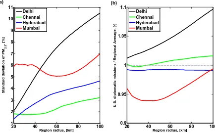
24-181
hour averaged PM2.5 concentrations (Fig. 2). The two cleanest air quality levels, ‘good’ and
182
‘satisfactory’, are defined as healthy, and the others (PM2.5 > 60 µg/m3) are defined as
183
unhealthy (CPCB, 2014). Delhi suffers the worst air quality among these cities, and the air
184
quality levels are categorized as ‘poor’, ‘very poor’ or ‘severe’ for ~50% of the time. These
185
hazy days mostly occur during October-February. The air quality in Chennai and Hyderabad
186
is much better than Delhi, with few ‘poor’ air-quality days; and ‘healthy’ days counted up to
9
50% of the time in Hyderabad and most of the time in Chennai. Mumbai has better air quality
188
than Delhi. This may be due to its coastal climate, where surface PM2.5 is often diluted by clean
189
air from the ocean. However, Mumbai still experiences about four months per year with air
190
quality of ‘poor’ standard or worse. The Diwali Fest and New Year festivals make the air
191
quality substantially worse in Delhi, as shown by the ‘severe’ days at the beginning of
192
November and January (Fig. 2a). This suggests that the fireworks during the festivals contribute
193
to an increase of PM2.5 loading in Delhi significantly. However, there is no clear festival effect
194
observed in the other three cities. It is unclear why no festival effect is observed in these other
195
cities, although it may reflect lower firework use and more favourable meteorological
196
conditions for dispersion in coastal cities.
197
All cities suffered severe episodes of poor air quality, with maximum hourly PM2.5
198
concentrations of 1676 µg/m3, 1334 µg/m3, 1107 µg/m3 and 758 µg/m3 in Delhi, Chennai,
199
Hyderabad and Mumbai, respectively. In Delhi, the maximum hourly PM2.5, observed during
200
the Diwali Fest nights in 2016 and 2018, is ~70% higher than the highest level recorded in
201
Beijing (980 µg/m3), China (San Martini et al., 2015; Wang et al., 2014; Zheng et al., 2015).
202
This strongly suggests that control of fireworks during the Diwali Fest would efficiently
203
mitigate short-term PM2.5 exposure in Delhi. This is also implied by a previous study (Singh et
204
al., 2010), where a significant increase in particle loading by a factor of 2-6 compared with the
205
period before and after Diwali Fest was found in Delhi during 2002-2007. Extreme episodes in
206
other cities were observed at night-time (10 p.m.-2 a.m.) from the end of October to the
207
beginning of December. The shallow planetary boundary layer (PBL) at night and intensive
208
crop burning in this season are the likely reasons for these extremely high concentrations
209
(Tiwari et al., 2013). Fig. S2 shows that there is a clear decrease in the frequency of high PM2.5
210
concentrations in all cities as the PBL height increases. We also observe an anti-correlation
211
between wind speed and PM2.5 loading. With the same PBL height, PM2.5 loading generally
10
decreases as wind speed increases, and PM2.5 is generally less than 100 µg/m3 when the wind
213
speed is greater than 4 m/s in all cities (Fig. S2). This is because the higher PBL and larger
214
wind speed dilute the surface PM2.5 (Chen et al., 2009; Mohan and Gupta, 2018).
215
In order to investigate the possible source regions of PM2.5 for each city, we analyse the
216
relationship between PM2.5 concentration and wind direction (Fig. 3). Delhi is influenced by
217
easterly and westerly/northwesterly winds, with high PM2.5 concentrations (>150 µg/m3) from
218
both directions. The westerly and northwesterly winds have the highest frequency (~33%) and
219
are associated with the most polluted episodes in Delhi. About 30% of the time PM2.5
220
concentration in Delhi are higher than 150 µg/m3, ~50% of which is associated with a westerly
221
or northwestly wind. This indicates that crop biomass burning and desert dust could be major
222
sources of PM2.5 in Delhi. Punjab and Haryana are located to the northwest of Delhi, and are
223
major sources of particles and gaseous precursors from crop burning during October-November
224
(Cusworth et al., 2018; Jethva et al., 2018; Rastogi et al., 2014), when the worst air quality is
225
observed in Delhi. Furthermore, previous modelling studies show significant increases (> 50%)
226
in aerosol loading when the westerly and northwesterly wind transports dust from the Thar
227
Desert to Delhi during April-June (Kumar et al., 2014a; Kumar et al., 2014b). In Hyderabad,
228
another inland city, the easterly/westerly wind pattern is also dominant. The easterly wind
229
brings a substantial amount of PM2.5 to Hyderabad, but the conditions are better than in Delhi,
230
with limited episodes of PM2.5 concentration higher than 150 µg/m3. Chennai and Mumbai are
231
coastal cities with a prevailing onshore wind for 70-80% of the time which brings relatively
232
clean marine air masses. The PM2.5 concentrations are generally lower than 75 µg/m3 when an
233
onshore wind is present. The offshore wind brings pollutants from inland regions to the cities,
234
but this occurs much less frequently (20-30%). These results indicate that there is a strong
235
interaction between meteorology and PM2.5 pollution, and strong local characteristics are found
11
in each city. Detailed investigation of these local characteristics would be helpful in tailoring
237
an effective mitigation policy for each city.
238
3.2 Seasonal and Diurnal Patterns of PM2.5
239
A distinct seasonal variation in the diurnal patterns is found, and this has different
240
characteristics in each city (Fig. 4). Generally, the climate in India is characterised by four
241
seasons: pre-monsoon/summer (March-May), monsoon (June-August), post-monsoon
242
(September-November) and winter (December-February). Notable inter-seasonal changes in
243
meteorology lead to significant differences in PM2.5 loading. Benefitting from the cleansing
244
effect of precipitation in the monsoon season (Ghosh et al., 2015), the hourly PM2.5 is generally
245
less than 50 µg/m3 in the inland cities (Delhi and Hyderabad) and less than 30 µg/m3 in the
246
coastal cities (Chennai and Mumbai). Apart from cleansing by precipitation, frequent deep
247
convection during summer monsoon in India can lift air pollutants near the surface to free
248
troposphere or even upper troposphere, as reported by previous modelling and observational
249
studies (Fadnavis et al., 2011; Kumar et al., 2015; Lelieveld et al., 2018). This transport process
250
dilutes air pollutants near the surface and could be one of the reasons that surface PM2.5
251
concentration is the lowest during the monsoon season. Future works, with aircraft
252
observations and modelling, are needed to quantify the relative importance of wash out and
253
vertical transport in reducing concentrations of surface pollutants. Chennai benefits from
254
prevailing onshore winds, with low PM2.5 loadings in both the pre-monsoon and monsoon
255
seasons (< 30 µg/m3). As a result of unfavourable meteorological conditions for dispersion and
256
an increase in emissions from heating (Guttikunda and Calori, 2013; Guttikunda and Gurjar,
257
2012), winter is the most polluted season in all cities. The slow wind speeds and shallow PBL
258
(Fig. S2) can trap PM2.5 in the surface layer and increase its concentration (Hu et al., 2019;
259
Zheng et al., 2015). The post-monsoon is the second most polluted season, with PM2.5 higher
12
than the annual averages. This inter-seasonal variation is consistent with the observations
261
during 2013-2016 (Sreekanth et al., 2018) despite the rapid increase of anthropogenic
262
emissions in India over the past decade (Li et al., 2017), indicating the importance of
263
meteorology on the seasonal variation.
264
A clear diurnal pattern is found in all cities during winter, post-monsoon and pre-monsoon
265
seasons (Fig. 4). However, no clear diurnal pattern is found during the monsoon season due to
266
the influence of precipitation. The minimum PM2.5 concentration during a day is generally
267
found at 3-4 p.m. local time, possibly resulting from the dilution effect of the fully developed
268
PBL in the afternoon (Fig. S3). PM2.5 concentrations peak during the morning rush hour in all
269
cities, the peaks approach 280 µg/m3 (Delhi), 90 µg/m3 (Chennai), 115 µg/m3 (Hyderabad) and
270
140 µg/m3 (Mumbai) in winter, respectively. It is interesting that the morning rush hour
271
consistently shifts 1-2 hours later from around 8 a.m. (pre-monsoon) to 10 a.m. (winter) in
272
Delhi and Mumbai, and to 9 a.m. (winter) in Chennai and Hyderabad. A remarkably strong
273
PM2.5 peak is found during morning rush hour in Chennai and Hyderabad, with hourly PM2.5
274
increased by ~50% and ~30% in two hours, respectively. However, only a slight increase in
275
PM2.5 concentration is observed in Delhi and Mumbai, with an increase of ~10% in winter.
276
These characteristics of PM2.5 variation during morning rush hour may be related to the size of
277
the population of each city. According to the latest census of India, there are around 4.6 and
278
7.0 million citizens in Chennai and Hyderabad, respectively; but more than 10 million citizens
279
in Delhi and Mumbai (India Office of the Registrar General and Census Commissioner, 2011).
280
Our results suggest that there is much greater human activity and emissions during the night in
281
these two larger megacities leading to higher night-time PM2.5 concentration but less variation
282
during the morning. The morning rush hour lasts longer until 10 a.m. in winter in these
283
megacities, in contrast to 9 a.m. in Chennai and Hyderabad. This is possibly because the busy
284
traffic, also alarger city size would prevent a smooth commute and lead to longer commuting
13
times (Alam and Ahmed, 2013; Srinivas, 2018). In addition, traffic is a major local source of
286
PM2.5 (~45%) in Delhi (Sahu et al., 2011). These results suggest that developing a more
287
convenient and efficient public transport system and encouraging the usage could be a key to
288
mitigate PM2.5 pollution, especially in the biggest cities. More work on source apportionment
289
is needed for each city to inform better targeted mitigation strategies.
290
291
3.3 Weekend Effect in Four Cities
292
We report the influence of a weekend effect on the diurnal patterns of PM2.5 in these cities,
293
as shown in Fig. 5. No noticeable weekend effect is found in Delhi and Hyderabad. This is
294
similar to Beijing and Chengdu in China (San Martini et al., 2015), with the diurnal patterns of
295
PM2.5 similar during weekdays and at the weekend. However, a notable weekend effect can be
296
found in Chennai and Mumbai. The difference in the diurnal pattern of PM2.5 between weekday
297
and weekend is greatest before 10 a.m. A stronger morning rush hour is found in Chennai and
298
Mumbai on weekdays, with ~10% higher PM2.5 than at the weekend. This indicates that the
299
decrease of traffic emissions in Mumbai and Chennai during weekend is probably the reason
300
of weekend effect, and control of traffic emissions could be an efficient measure for improving
301
air quality. In Chennai, PM2.5 concentrations are about 5 µg/m3 higher during night (12-5 a.m.)
302
at the weekend than on weekdays; in contrast, PM2.5 concentration is about 5 µg/m3 lower at
303
the weekend in Mumbai. These different weekend effects possibly indicate different life styles
304
and PM2.5 sources in each city. Further modelling and emission flux studies are needed to better
305
understand the sources of PM2.5 in each city.
306
3.4 Exposure to PM2.5 and Health Impacts
14
We use these long-term in-situ observations to estimate the exposure of the population to
308
PM2.5 in Delhi, Chennai, Hyderabad and Mumbai. The annual averaged PM2.5 loading in these
309
cities is 110 µg/m3, 33 µg/m3, 56 µg/m3 and 60 µg/m3, respectively. The population-weighted
310
annual mean PM2.5 loading is 72 µg/m3 across the four cities, which is about 3.5 times higher
311
than the global population-weighted value (20 µg/m3, van Donkelaar et al., 2010) and ~22%
312
higher than average Chinese city-level value (Zhang and Cao, 2015). The annual averaged
313
PM2.5 loading in Delhi is much higher than all Chinese major cities in the last five years (Wang
314
et al., 2019). Fig. 6 shows the time integrated exposure, which indicates the proportion of time
315
that a citizen is exposed to PM2.5 concentrations over a given level over the four years
316
measurement period. Citizens are exposed to unhealthy air quality (PM2.5 > 60 µg/m3) for about
317
70% (Delhi), 15% (Chennai), 50% (Hyderabad) and 45% (Mumbai) of the time. The air quality
318
is especially unhealthy in Delhi where citizens are exposed to ‘severe’ PM2.5 pollution (>250
319
µg/m3) for about 10% of the time. It is noteworthy that citizens of all four cities are exposed to
320
air quality exceeding the 10 µg/m3 WHO guideline nearly 100% of the time. PM2.5 in all the
321
cities except Chennai severely exceeds the revised Indian NAAQS standards of an annual
322
average of 40 µg/m3.
323
These continuous in-situ measurements give us an opportunity to make a robust
324
assessment of term health impacts on a city scale in India (Fig. 7). We estimate that
long-325
term ambient PM2.5 exposure causes 10,200 (95% confidence interval: 6,800–14,300), 2,800
326
(1,500–4,100), 5,200 (3,100–7,400), and 9,500 (5,800–13,600) premature mortality each year
327
in Delhi, Chennai, Hyderabad, and Mumbai, respectively. Our premature mortality estimate
328
for Delhi is reasonably agreed (~10% negative bias) with a previous estimate from the
329
GBD2016 (GBD, 2016). We estimate that about 248,000 (168,000–340,700), 66,000 (37,400–
330
96,800), 125,000 (78,300–176,100), and 230,000 (145,200–321,700) years of life are lost each
331
year in Delhi, Chennai, Hyderabad, and Mumbai, respectively. The annual mortality rate per
15
100,000 population, which is independent of population size, is 93 (62–130), 60 (33–89), 74
333
(45–106), 76 (46–108) in Delhi, Chennai, Hyderabad, and Mumbai, respectively.
334
Cardiovascular disease dominates the disease burden, with ischaemic heart disease (IHD)
335
contributing ~40% and cerebrovascular disease (CEV) contributing ~30% in each city.
336
We estimate the health risks of short-term exposure during the New Year and Diwali Fest
337
in Delhi and provide quantitative evidence to support control of fireworks. The fireworks
338
during New Year enhance the PM2.5 pollution in Delhi to some extent. The averaged PM2.5
339
concentration during 1-3 January (276 µg/m3) was about 20% higher than the monthly average
340
of January (227 µg/m3). This makes the daily premature mortality in Delhi slightly increase
341
from January average of 43 (24-59) person per day to 50 (28-67) person per day during the
342
New Year. The fireworks during Diwali Fest contribute substantially to the extremely high
343
hourly concentration of PM2.5 in Delhi (up to 1676 µg/m3), leading to hazardous short-term
344
exposure. Crop burning in Punjab and Haryana makes a large contribution to PM2.5 loading in
345
Delhi during October-November (Cusworth et al., 2018; Jethva et al., 2018), while fireworks
346
in Diwali Fest can greatly worsen PM2.5 pollution over the period of a few days (Singh et al.,
347
2010). We find that the PM2.5 concentration during Diwali Fest (including the festival start day
348
and the following two days) is 75% higher (~320 µg/m3) than the two-month average (~183
349
µg/m3 in October-November) in Delhi over this four-year period. We estimate the short-term
350
health impacts from ambient PM2.5 concentrations during Diwali Fest at 56 (32-75) premature
351
mortality per day in Delhi. This is an additional 20 (13-25) daily premature mortality, an
352
increase of 56% compared with the October-November average of 36 (19–50) daily premature
353
mortality. This highlights the importance of reducing firework emissions during Diwali Fest to
354
improve public health.
355
3.5 Spatial Representativeness and Uncertainty
16
In order to analyse the spatial representativeness of observations in U.S. diplomatic
357
missions in each city and the corresponding uncertainty, we extract surface PM2.5
358
concentrations from a global high spatial resolution satellite-retrieved dataset (van Donkelaar
359
et al., 2015, http://fizz.phys.dal.ca/~atmos/martin/?page_id=140). The extracted dataset
360
includes the annual averaged (2015-2016) PM2.5 concentration at locations of U.S. diplomatic
361
missions and their surrounding regions within a distance of 20-100 km. This satellite-retrieved
362
dataset is of high horizontal-resolution of 0.01 deg. × 0.01 deg. (lat-lon, about 1km × 1km).
363
The retrieved data has been validated and widely adopted for global health effect analysis in
364
previous studies (van Donkelaar et al., 2010; van Donkelaar et al., 2015). The standard
365
deviation and ratios of PM2.5 concentrations between U.S. diplomatic missions’ locations and
366
averages of surrounding regions are given in Fig. 8.
367
As shown in Fig. 8, the uncertainty in Chennai and Hyderabad is negligible, with
368
difference between U.S. diplomatic missions and surrounding regions less than 5%, and the
369
standard deviations increase slowly with the increase of distance from U.S. diplomatic missions
370
but always less than 5%. This indicates a relatively homogeneous spatial distribution of PM2.5
371
concentrations in Chennai and Hyderabad. In Mumbai, the standard deviation varies between
372
5-7%, with the minimum at a distance of ~60 km. This may be due to the influence of nearby
373
large cities, such as Pune which is about 100 km away from Mumbai. The difference between
374
U.S. diplomatic mission in Mumbai and the surrounding regional average is less than 6% in
375
general, with the maximum underestimation of ~6% when the distance is about 40 km. This
376
indicates that the observations of U.S. diplomatic mission in Mumbai well represent the nearby
377
region, at least the region within 100 km. The representativeness of observations in the U.S.
378
Embassy of Delhi decreases as the distance increases. The U.S. Embassy’s observations may
379
overestimate the PM2.5 concentrations in Delhi compared with the regional average, but this
380
overestimation is less than 5% and with standard deviations less than 6% when the distance (or
17
region radius) is less than 60 km. However, the overestimation increases to ~10% with a
382
standard deviation of ~10% when the distance is 100 km. This indicates a good
383
representativeness of U.S. Embassy’s observation for Delhi and its surrounding region within
384
60 km, but may overestimate the PM2.5 concentration and the corresponding human exposure
385
by ~10% if using U.S. Embassy’s observations to estimate the PM2.5 human exposure in a
386
larger region of Delhi, such as with a radius of 100 km. This could be due to the higher
387
urbanization level of Delhi, leading to a higher pollution level in/near the city center.
388
389
4. Conclusions and Discussion
390
This study has estimated the health risks of long-term exposure to PM2.5 based on in-situ
391
observations in four Indian megacities (Delhi, Hyderabad, Chennai and Mumbai) during
2015-392
2018, and quantified the health risks of short-term exposure during Diwali Fest in Delhi for the
393
first time. We also summarized the local characteristics of seasonal and diurnal variations of
394
PM2.5, and report the influence of a weekend effect on diurnal patterns. The results from this
395
study are valuable for modelling studies and helpful in tailoring city-specific mitigation
396
strategies.
397
Generally, substantial inter-seasonal variations in PM2.5 are observed in the four cities,
398
with the highest concentration during winter and the lowest during the monsoon season, when
399
intensive wet scavenging lowers pollutant concentrations (Naja et al., 2014; Ojha et al., 2012).
400
Winter is the most polluted season as a consequence of the shallow PBL and increased
401
emissions from heating (Guttikunda and Calori, 2013; Guttikunda and Gurjar, 2012). Solid fuel
402
burning is a common form of household heating in winter over India (Dumka et al., 2019;
403
Jagadish and Dwivedi, 2018). To increase the efficiency of energy use and reduce PM2.5
404
emissions in cities, we would suggest reduction in use of solid fuels (e.g., replace wood and
18
coal with liquid petroleum gas or compressed natural gas) and implementation of
406
central/electric heating systems with heating centres located in non-upwind regions (e.g., north
407
or south of Delhi). The megacities of Delhi and Mumbai show a weak morning rush hour effect,
408
but there is a strong one in Hyderabad and Chennai. For the first time, we report an interesting
409
and consistent shift of about two hours in the timing of the morning rush hour from
pre-410
monsoon/summer (8 a.m.) to winter (9-10 a.m.), and analyse the influence of a weekend effect
411
on the diurnal patterns of PM2.5 in Indian megacities. The coastal cities of Chennai and Mumbai
412
show a clear difference in morning PM2.5 concentrations between weekdays and the weekend,
413
but no noticeable difference was observed in the inland cities of Delhi and Hyderabad. These
414
results indicate traffic emissions could be important sources of PM2.5 and highlight the distinct
415
local characteristics of human activity in each city, which is critical information for modelling
416
studies. The four cities show significant differences in wind patterns and transport of PM2.5,
417
suggesting that different control strategies are needed for each city that take into account its
418
local emission characteristics and meteorological conditions.
419
In this study, we report the high health risks of exposure to PM2.5pollution in Indian cities
420
and highlight hazardous short-term exposure during Diwali Fest in Delhi. Across the four cities,
421
long-term exposure to PM2.5 causes about 28,000 (95% confidence interval: 17,200–39,400)
422
premature mortality and 670,000 (428,900–935,200) years of life lost each year. Fireworks
423
during the Diwali Fest lead to severe air pollution in Delhi, and this is responsible for 56
(32-424
75) premature mortality per day, a 56% increase over the monthly average. More effective
425
control policies are urgently required to mitigate the health burden and achieve sustainable
426
development. Previous studies have shown that the dominant emission sources contributing to
427
the disease burden from ambient PM2.5 exposure are land transport in Delhi, residential solid
428
fuel burning in Chennai and Hyderabad, and industrial coal burning in Mumbai (Conibear et
429
al., 2018a). The disease burden is likely to increase substantially in future due to population
19
ageing and growth, which enhance the susceptibility to disease, unless stringent emission
431
control policies are implemented (Conibear et al., 2018b).
432
We have estimated the PM2.5 exposure in the four cities with continuous observations, but
433
it is noteworthy that some other Indian cities experience more severe air pollution (WHO,
434
2016). Continuous, widespread pollutant measurements across India would provide more
435
complete information on regional pollutant characteristics and overall pollutant levels. More
436
detailed measurements of the physicochemical properties of PM2.5 in major cities, e.g., their
437
composition and size distribution, would permit better characterisation of urban sources, and
438
provide the information needed to design appropriate mitigation strategies.
439
440
Author contributions
441
Y. C. and O. W. conceived the study. Y. C. performed the analysis and interpreted the results with
442
input from all co-authors. L. C. helped with the health effect assessment. The manuscript was written with
443
input from all co-authors.
444
Additional Information
445
The authors declare no competing financial interest.
446
Acknowledgments
447
Hourly measurements of PM2.5 made at U.S. diplomatic missions in India are available through the
448
AirNow platform maintained by the U.S. Department of State and the U.S. Environmental Protection Agency
449
at https://www.airnow.gov/. Meteorological variables are available through the Integrated Surface
450
Database—Surface Data Hourly Global data product maintained by the U.S. National Oceanic and
451
Atmospheric Administration—National Climatic Data Center at https://www.ncdc.noaa.gov/. Y. W. would
452
like to thank the China Scholarship Council for support through a PhD scholarship. Y. C. and O. W. would
453
like to thank the NERC for funding (NE/P01531X/1 and NE/N006976/1). R. L. would like to thank the
454
National Natural Science Foundation of China (grant no. 41305114). L. C. would like to thank the N8
20
consortium and EPSRC (grant EP/K000225/1). The paper is based on interpretation of scientific results and
456
in no way reflect the viewpoint of the funding agencies.
21
References:
Alam, M.A., Ahmed, F., 2013. URBAN TRANSPORT SYSTEMS AND CONGESTION: A CASE STUDY OF INDIAN CITIES. Transport and Communications Bulletin for Asia and the Pacific 82.
Atkinson, R.W., Kang, S., Anderson, H.R., Mills, I.C., Walton, H.A., 2014. Epidemiological time series studies of PM<sub>2.5</sub> and daily mortality and hospital admissions: a systematic review and meta-analysis. Thorax 69, 660-665.
Burnett Richard, T., Pope, C.A., Ezzati, M., Olives, C., Lim Stephen, S., Mehta, S., Shin Hwashin, H., Singh, G., Hubbell, B., Brauer, M., Anderson, H.R., Smith Kirk, R., Balmes John, R., Bruce Nigel, G., Kan, H., Laden, F., Prüss-Ustün, A., Turner Michelle, C., Gapstur Susan, M., Diver, W.R., Cohen, A., 2014. An Integrated Risk Function for Estimating the Global Burden of Disease Attributable to Ambient Fine Particulate Matter Exposure. Environmental Health Perspectives 122, 397-403. Chen, Y., Zhao, C., Zhang, Q., Deng, Z.Z., Huang, M.Y., Ma, X.C., 2009. Aircraft study of mountain
chimney effect of Beijing, china. Journal of Geophysical Research: Atmospheres 114.
Chowdhury, S., Dey, S., 2016. Cause-specific premature death from ambient PM2.5 exposure in India: Estimate adjusted for baseline mortality. Environment International 91, 283-290.
Chowdhury, S., Dey, S., Smith, K.R., 2018. Ambient PM2.5 exposure and expected premature mortality to 2100 in India under climate change scenarios. Nature Communications 9, 318.
Chowdhury, S., Dey, S., Tripathi, S.N., Beig, G., Mishra, A.K., Sharma, S., 2017. “Traffic intervention” policy fails to mitigate air pollution in megacity Delhi. Environmental Science & Policy 74, 8-13. Conibear, L., Butt, E.W., Knote, C., Arnold, S.R., Spracklen, D.V., 2018a. Residential energy use emissions
dominate health impacts from exposure to ambient particulate matter in India. Nature Communications 9, 617.
Conibear, L., Butt, E.W., Knote, C., Arnold, S.R., Spracklen, D.V., 2018b. Stringent Emission Control Policies Can Provide Large Improvements in Air Quality and Public Health in India. GeoHealth 2, 196-211.
CPCB, 2009. National Ambient Air Quality Standards. Central Pollution Control Board, New Delhi, India. CPCB, 2014. National Air Quality Index Report, Central Pollution Control Board, New Delhi, India.,
https://app.cpcbccr.com/AQI_India/ (last access: 25.01.2019).
Crippa, P., Castruccio, S., Archer-Nicholls, S., Lebron, G.B., Kuwata, M., Thota, A., Sumin, S., Butt, E., Wiedinmyer, C., Spracklen, D.V., 2016. Population exposure to hazardous air quality due to the 2015 fires in Equatorial Asia. Scientific Reports 6, 37074.
Cusworth, D.H., Mickley, L.J., Sulprizio, M.P., Liu, T., Marlier, M.E., DeFries, R.S., Guttikunda, S.K., Gupta, P., 2018. Quantifying the influence of agricultural fires in northwest India on urban air pollution in Delhi, India. Environmental Research Letters 13, 044018.
Dumka, U.C., Tiwari, S., Kaskaoutis, D.G., Soni, V.K., Safai, P.D., Attri, S.D., 2019. Aerosol and pollutant characteristics in Delhi during a winter research campaign. Environmental Science and Pollution Research 26, 3771-3794.
EPA, 2009. Standard operating procedure for the continuous measurement of particulate matter. (last access: 8 Nov. 2018).
EPA, 2015. List of designated reference and equivalent methods. (last access: 20 Nov. 2018).
Fadnavis, S., Buchunde, P., Ghude, S.D., Kulkarni, S.H., Beig, G., 2011. Evidence of seasonal enhancement of CO in the upper troposphere over India. International Journal of Remote Sensing 32, 7441-7452. Gao, M., Beig, G., Song, S., Zhang, H., Hu, J., Ying, Q., Liang, F., Liu, Y., Wang, H., Lu, X., Zhu, T., Carmichael, G.R., Nielsen, C.P., McElroy, M.B., 2018a. The impact of power generation emissions on ambient PM2.5 pollution and human health in China and India. Environment International 121, 250-259.
Gao, M., Han, Z., Liu, Z., Li, M., Xin, J., Tao, Z., Li, J., Kang, J.E., Huang, K., Dong, X., Zhuang, B., Li, S., Ge, B., Wu, Q., Cheng, Y., Wang, Y., Lee, H.J., Kim, C.H., Fu, J.S., Wang, T., Chin, M., Woo, J.H., Zhang, Q., Wang, Z., Carmichael, G.R., 2018b. Air quality and climate change, Topic 3 of the Model Inter-Comparison Study for Asia Phase III (MICS-Asia III) – Part 1: Overview and model evaluation. Atmos. Chem. Phys. 18, 4859-4884.
22
GBD, 2016. Global, regional, and national comparative risk assessment of 84 behavioural, environmental and occupational, and metabolic risks or clusters of risks, 1990–2016: a systematic analysis for the Global Burden of Disease Study 2016. The Lancet 390 1345-1422.
GBD, 2017a. Global Burden of Disease Study 2016 (GBD 2016) Population Estimates 1950-2016.
http://ghdx.healthdata.org/record/global-burden-disease-study-2016-gbd-2016-population-estimates-1950-2016 (last access: 2025.2001.2019).
GBD, 2017b. Global Burden of Disease Study 2016 (GBD 2016) Reference Life Table.
http://ghdx.healthdata.org/record/global-burden-disease-study-2016-gbd-2016-reference-life-table
(lase access: 2025.2001.2019).
GBD, 2018. Institute for Health Metrics and Evaluation: GBD Compare Data Visualization. vizhub.healthdata.org/gbd-compare (lase access: 25.01.2019).
Ghosh, S., Biswas, J., Guttikunda, S., Roychowdhury, S., Nayak, M., 2015. An investigation of potential regional and local source regions affecting fine particulate matter concentrations in Delhi, India. Journal of the Air & Waste Management Association 65, 218-231.
Guttikunda, S.K., Calori, G., 2013. A GIS based emissions inventory at 1 km × 1 km spatial resolution for air pollution analysis in Delhi, India. Atmospheric Environment 67, 101-111.
Guttikunda, S.K., Gurjar, B.R., 2012. Role of meteorology in seasonality of air pollution in megacity Delhi, India. Environmental Monitoring and Assessment 184, 3199-3211.
Héroux, M.-E., Anderson, H.R., Atkinson, R., Brunekreef, B., Cohen, A., Forastiere, F., Hurley, F., Katsouyanni, K., Krewski, D., Krzyzanowski, M., Künzli, N., Mills, I., Querol, X., Ostro, B., Walton, H., 2015. Quantifying the health impacts of ambient air pollutants: recommendations of a WHO/Europe project. International Journal of Public Health 60, 619-627.
Hu, D., Chen, Y., Wang, Y., Daële, V., Idir, M., Yu, C., Wang, J., Mellouki, A., 2019. Photochemical reaction playing a key role in particulate matter pollution over Central France: Insight from the aerosol optical properties. Science of The Total Environment 657, 1074-1084.
Huang, J., Pan, X., Guo, X., Li, G., 2018. Health impact of China's Air Pollution Prevention and Control Action Plan: an analysis of national air quality monitoring and mortality data. The Lancet Planetary Health 2, e313-e323.
India Office of the Registrar General and Census Commissioner, 2011. Census of India, Minist. of Home Affairs, Gov. of India, New Delhi.
Jagadish, A., Dwivedi, P., 2018. In the hearth, on the mind: Cultural consensus on fuelwood and cookstoves in the middle Himalayas of India. Energy Research & Social Science 37, 44-51.
Jethva, H., Chand, D., Torres, O., Gupta, P., Lyapustin, A., Patadia, F., 2018. Agricultural Burning and Air Quality over Northern India: A Synergistic Analysis using NASA’s A-train Satellite Data and Ground Measurements. Aerosol and Air Quality Research 18, 1756-1773.
Jiang, J., Zhou, W., Cheng, Z., Wang, S., He, K., Hao, J., 2015. Particulate Matter Distributions in China during a Winter Period with Frequent Pollution Episodes (January 2013). Aerosol and Air Quality Research 15, 494-503.
Kumar, R., Barth, M.C., Madronich, S., Naja, M., Carmichael, G.R., Pfister, G.G., Knote, C., Brasseur, G.P., Ojha, N., Sarangi, T., 2014a. Effects of dust aerosols on tropospheric chemistry during a typical pre-monsoon season dust storm in northern India. Atmos. Chem. Phys. 14, 6813-6834.
Kumar, R., Barth, M.C., Pfister, G.G., Nair, V.S., Ghude, S.D., Ojha, N., 2015. What controls the seasonal cycle of black carbon aerosols in India? Journal of Geophysical Research: Atmospheres 120, 7788-7812.
Kumar, R., Barth, M.C., Pfister, G.G., Naja, M., Brasseur, G.P., 2014b. WRF-Chem simulations of a typical pre-monsoon dust storm in northern India: influences on aerosol optical properties and radiation budget. Atmos. Chem. Phys. 14, 2431-2446.
Lelieveld, J., Bourtsoukidis, E., Brühl, C., Fischer, H., Fuchs, H., Harder, H., Hofzumahaus, A., Holland, F., Marno, D., Neumaier, M., Pozzer, A., Schlager, H., Williams, J., Zahn, A., Ziereis, H., 2018. The South Asian monsoon—Pollution pump and purifier. Science.
Lelieveld, J., Evans, J.S., Fnais, M., Giannadaki, D., Pozzer, A., 2015. The contribution of outdoor air pollution sources to premature mortality on a global scale. Nature 525, 367.
23
Li, C., McLinden, C., Fioletov, V., Krotkov, N., Carn, S., Joiner, J., Streets, D., He, H., Ren, X., Li, Z., Dickerson, R.R., 2017. India Is Overtaking China as the World’s Largest Emitter of Anthropogenic Sulfur Dioxide. Scientific Reports 7, 14304.
Liu, D., Quennehen, B., Darbyshire, E., Allan, J.D., Williams, P.I., Taylor, J.W., Bauguitte, S.J.B., Flynn, M.J., Lowe, D., Gallagher, M.W., Bower, K.N., Choularton, T.W., Coe, H., 2015. The importance of Asia as a source of black carbon to the European Arctic during springtime 2013. Atmos. Chem. Phys. 15, 11537-11555.
Lv, B., Cai, J., Xu, B., Bai, Y., 2017. Understanding the Rising Phase of the PM2.5 Concentration Evolution in Large China Cities. Scientific Reports 7, 46456.
Lv, B., Liu, Y., Yu, P., Zhang, B., Bai, Y., 2015. Characterizations of PM2. 5 pollution pathways and sources analysis in four large cities in China. Aerosol Air Qual. Res 15, 1836-1843.
Marrapu, P., Cheng, Y., Beig, G., Sahu, S., Srinivas, R., Carmichael, G.R., 2014. Air quality in Delhi during the Commonwealth Games. Atmos. Chem. Phys. 14, 10619-10630.
Mohan, M., Gupta, M., 2018. Sensitivity of PBL parameterizations on PM10 and ozone simulation using chemical transport model WRF-Chem over a sub-tropical urban airshed in India. Atmospheric Environment 185, 53-63.
Mukherjee, A., Toohey, D.W., 2016. A study of aerosol properties based on observations of particulate matter from the U.S. Embassy in Beijing, China. Earth's Future 4, 381-395.
Naja, M., Mallik, C., Sarangi, T., Sheel, V., Lal, S., 2014. SO2 measurements at a high altitude site in the central Himalayas: Role of regional transport. Atmospheric Environment 99, 392-402.
Ojha, N., Naja, M., Singh, K.P., Sarangi, T., Kumar, R., Lal, S., Lawrence, M.G., Butler, T.M., Chandola, H.C., 2012. Variabilities in ozone at a semi-urban site in the Indo-Gangetic Plain region: Association with the meteorology and regional processes. Journal of Geophysical Research: Atmospheres 117.
Pope, C.A., Ezzati, M., Dockery, D.W., 2009. Fine-Particulate Air Pollution and Life Expectancy in the United States. New England Journal of Medicine 360, 376-386.
Rastogi, N., Singh, A., Singh, D., Sarin, M.M., 2014. Chemical characteristics of PM2.5 at a source region of biomass burning emissions: Evidence for secondary aerosol formation. Environmental Pollution 184, 563-569.
Sahu, S.K., Beig, G., Parkhi, N.S., 2011. Emissions inventory of anthropogenic PM2.5 and PM10 in Delhi during Commonwealth Games 2010. Atmospheric Environment 45, 6180-6190.
Sahu, S.K., Kota, S.H., 2017. Significance of PM2.5 Air Quality at the Indian Capital. Aerosol and Air Quality Research 17, 588-597.
San Martini, F.M., Hasenkopf, C.A., Roberts, D.C., 2015. Statistical analysis of PM2.5 observations from diplomatic facilities in China. Atmospheric Environment 110, 174-185.
Schnell, J.L., Naik, V., Horowitz, L.W., Paulot, F., Mao, J., Ginoux, P., Zhao, M., Ram, K., 2018. Exploring the relationship between surface PM2.5 and meteorology in Northern India. Atmos. Chem. Phys. 18, 10157-10175.
Sharma, M., Dixit, O., 2016. Comprehensive Study on Air Pollution and Green House Gases (GHGs) in Delhi. . DPCC.
Sharma, S.K., Mandal, T.K., Sharma, A., Jain, S., Saraswati, 2018. Carbonaceous Species of PM2.5 in Megacity Delhi, India During 2012–2016. Bulletin of Environmental Contamination and Toxicology 100, 695-701.
Singh, D.P., Gadi, R., Mandal, T.K., Dixit, C.K., Singh, K., Saud, T., Singh, N., Gupta, P.K., 2010. Study of temporal variation in ambient air quality during Diwali festival in India. Environmental Monitoring and Assessment 169, 1-13.
Sreekanth, V., Mahesh, B., Niranjan, K., 2018. Gradients in PM2.5 over India: Five city study. Urban Climate 25, 99-108.
Srinivas, A., 2018. How traffic flow affects travel time in Delhi and Mumbai. livemint.
Tiwari, S., Srivastava, A.K., Bisht, D.S., Parmita, P., Srivastava, M.K., Attri, S.D., 2013. Diurnal and seasonal variations of black carbon and PM2.5 over New Delhi, India: Influence of meteorology. Atmospheric Research 125-126, 50-62.
24
van Donkelaar, A., Martin, R.V., Brauer, M., Boys, B.L., 2015. Use of Satellite Observations for Long-Term Exposure Assessment of Global Concentrations of Fine Particulate Matter. Environmental Health Perspectives 123, 135-143.
van Donkelaar, A., Martin, R.V., Levy, R.C., da Silva, A.M., Krzyzanowski, M., Chubarova, N.E., Semutnikova, E., Cohen, A.J., 2011. Satellite-based estimates of ground-level fine particulate matter during extreme events: A case study of the Moscow fires in 2010. Atmospheric Environment 45, 6225-6232.
Wang, J., Xing, J., Mathur, R., Pleim Jonathan, E., Wang, S., Hogrefe, C., Gan, C.-M., Wong David, C., Hao, J., 2017. Historical Trends in PM2.5-Related Premature Mortality during 1990–2010 across the Northern Hemisphere. Environmental Health Perspectives 125, 400-408.
Wang, Y., Chen, Y., 2019. Significant Climate Impact of Highly Hygroscopic Atmospheric Aerosols in Delhi, India. Geophysical Research Letters 0.
Wang, Y., Li, W., Gao, W., Liu, Z., Tian, S., Shen, R., Ji, D., Wang, S., Wang, L., Tang, G., Song, T., Cheng, M., Wang, G., Gong, Z., Hao, J., Zhang, Y., 2019. Trends in particulate matter and its chemical compositions in China from 2013–2017. Science China Earth Sciences.
Wang, Y., Yao, L., Wang, L., Liu, Z., Ji, D., Tang, G., Zhang, J., Sun, Y., Hu, B., Xin, J., 2014. Mechanism for the formation of the January 2013 heavy haze pollution episode over central and eastern China. Science China Earth Sciences 57, 14-25.
West, J.J., Szopa, S., Hauglustaine, D.A., 2007. Human mortality effects of future concentrations of tropospheric ozone. Comptes Rendus Geoscience 339, 775-783.
WHO, 2013. Health risks of air pollution in Europe – HRAPIE project: Recommendations for concentration– response functions for cost–benefit analysis of particulate matter, ozone and nitrogen dioxide.
http://www.euro.who.int/__data/assets/pdf_file/0006/238956/Health_risks_air_pollution_HRAPIE _project.pdf?ua=238951 (last access: 238925.238901.232019).
WHO, 2016. WHO Global Urban Ambient Air Pollution Database (update 2016). Available:
http://www.who.int/airpollution/data/cities-2016/en/,, (last access: 08 Nov. 2018).
Yu, P., Rosenlof, K.H., Liu, S., Telg, H., Thornberry, T.D., Rollins, A.W., Portmann, R.W., Bai, Z., Ray, E.A., Duan, Y., Pan, L.L., Toon, O.B., Bian, J., Gao, R.-S., 2017. Efficient transport of tropospheric aerosol into the stratosphere via the Asian summer monsoon anticyclone. Proceedings of the National Academy of Sciences 114, 6972-6977.
Zhang, Y.-L., Cao, F., 2015. Fine particulate matter (PM2.5) in China at a city level. Scientific Reports 5, 14884.
Figure 1. Map of Delhi, Chennai, Hyderabad and Mumbai. Surface annual (2015) average of
PM2.5 is retrieved from satellite observations with sea-salt and dust excluded and at a relative
[image:25.595.125.484.133.480.2]Figure 2.Calendar-view of daily PM2.5 air quality levels averaged over 2015-2018. (a) Delhi,
(b) Chennai, (c) Hyderabad, and (d) Mumbai. The air quality levels are categorized following the
Indian national air quality index definitions (https://app.cpcbccr.com/AQI_India).
Figure 3.Frequency distributions of PM2.5 concentration as a function of wind direction. (a)
Delhi, (b) Chennai, (c) Hyderabad, and (d) Mumbai.
20% 15% 10% 5%
W E
S N
0 - 35 35 - 75 75 - 115 115 - 150 150 - 250 250 - 500 Delhi PM
2.5 [g/m 3
]
20% 15% 10% 5%
W E
S N
0 - 35 35 - 75 75 - 115 115 - 150 150 - 250 250 - 500 Chennai PM
2.5 [g/m 3
]
20% 15% 10% 5%
W E
S N
0 - 35 35 - 75 75 - 115 115 - 150 150 - 250 250 - 500 Hyderabad PM
2.5 [g/m 3]
20% 15% 10% 5%
W E
S N
0 - 35 35 - 75 75 - 115 115 - 150 150 - 250 250 - 500 Mumbai PM
2.5 [g/m 3]
(a) (b)
(c) (d)
(a) (b)
[image:26.595.112.473.458.697.2]Figure 4. Average diurnal variation of PM2.5 concentrations for each season. (a) Delhi, (b)
Chennai, (c) Hyderabad, and (d) Mumbai. The statistical values for each city in each season,
including average, median, 75% percentile, 25% percentile, 95% percentile and 5% percentile, are
[image:27.595.79.489.76.313.2]given in Fig. S4-S8.
Figure 5.Average diurnal variation of PM2.5 concentrations on weekdays and at the weekend.
(a) Delhi, (b) Chennai, (c) Hyderabad, and (d) Mumbai.
0 5 10 15 20
50 100 150 200
Delhi
Local Time, [hour]
PM 2 .5 , [ g /m 3 ]
0 5 10 15 20
20 40 60 80
Chennai
Local Time, [hour]
PM 2 .5 , [ g /m 3 ] Winter Pre-monsoon Monsoon Post-monsoon Annual average
0 5 10 15 20
40 60 80 100
Hyderabad
Local Time, [hour]
PM 2 .5 , [ g /m 3 ]
0 5 10 15 20
40 60 80 100 120 140 Mumbai
Local Time, [hour]
PM 2 .5 , [ g /m 3 ]
0 5 10 15 20
80 100 120
Delhi
Local Time, [hour]
PM 2 .5 , [ g /m 3 ] Weekend Weekday Average
0 5 10 15 20
30 35 40 45
Chennai
Local Time, [hour]
PM 2 .5 , [ g /m 3 ]
0 5 10 15 20
45 50 55 60 65 70 Hyderabad
Local Time, [hour]
PM 2 .5 , [ g /m 3 ]
0 5 10 15 20
50 60 70
Mumbai
Local Time, [hour]
PM 2 .5 , [ g /m 3 ]
(a) (b)
(c) (d)
(a) (b)
[image:27.595.79.488.472.707.2]Figure 7. Annual city-specific disease burden from long-term ambient PM2.5 exposure. (a)
Mortality rate per 100,000 population. (b) Premature mortality per disease of chronic obstructive
pulmonary disease (COPD), lower respiratory infection (LRI), ischaemic heart disease (IHD),
cerebrovascular disease (CEV), and lung cancer (LC). (c) Years of life lost.
(a)
(b)
Fig. 8. Spatial representativeness of U.S. diplomatic mission observations in each city. (a) Standard deviation of PM2.5 mass concentrations in surrounding region as a function of region
radius. (b) The ratio between U.S. diplomatic mission observation and regional average as a
function of region radius.
20 40 60 80 100
1 2 3 4 5 6 7 8 9 10 11 Sta n d a rd d e v ia ti o n o f PM 2.5 , [% ]
Region radius, [km]
(a)
Delhi Chennai Hyderabad Mumbai
20 40 60 80 100
0.9 0.95 1 1.05 1.1 U .S. d ip lo m a ti c m is s io n s / R e g io n a l A v e ra g e , [-]
Region radius, [km]
(b)
S1
Supporting Information
for
Local Characteristics of and Exposure to Fine Particulate Matter (PM
2.5) in
Four Indian Megacities
Ying Chen1*, Oliver Wild1, Luke Conibear2,Liang Ran3, Jianjun He4, Lina Wang5, Yu Wang6
1Lancaster Environment Centre, Lancaster University, Lancaster, LA1 4YQ, UK
2Institute for Climate and Atmospheric Science, School of Earth and Environment, University of Leeds, UK.
3Key Laboratory of Middle Atmosphere and Global Environment Observation, Institute of Atmospheric Physics, Chinese
Academy of Sciences, Beijing, 100029, China
4State Key Laboratory of Severe Weather & Key Laboratory of Atmospheric Chemistry of CMA, Chinese Academy of
Meteorological Sciences, Beijing, 100081, China
5Shanghai Key Laboratory of Atmospheric Particle Pollution and Prevention, Department of Environmental Science and
Engineering, Fudan University, Shanghai 200433, China
6Centre for Atmospheric Sciences, School of Earth and Environmental Sciences, University of Manchester, Manchester, UK
Correspondence to: Ying Chen (y.chen65@lancaster.ac.uk)
Contents of this file
Tables:
Table S1 – Overview of PM2.5 observations in four cities.
Figures:
Figure S1 – Monthly statistical overview of hourly PM2.5 concentrations.
Figure S2 – Hourly PM2.5 concentration as a function of PBL height and wind speed.
Figure S3 – The averaged diurnal pattern of PBL for each season.
Figure S4 – The annual averaged diurnal pattern of PM2.5 in each city.
Figure S5 – The winter averaged diurnal pattern of PM2.5 in each city.
Figure S6 – The pre-monsoon averaged diurnal pattern of PM2.5 in each city.
Figure S7 – The post-monsoon averaged diurnal pattern of PM2.5 in each city.