RESEARCH ARTICLE
HYDROLOGICAL IMPACTS OF LAND COVER CHANGES IN UPPER ATHI RIVER
CATCHMENT, KENYA
*Katana, S. J. S., Munyao, T. M. and Ucakuwun, E. K.
School of Environmental Studies, University of Eldoret, P. O. Box 1125-30100, Eldoret, Kenya
ARTICLE INFO ABSTRACT
Land cover changes have significant impacts on hydrological processes at the watershed level. The objective of the study was to apply a rainfall-runoff model derived using Hydrologic Engineering Centre-Hydrologic Modeling System (HEC-HMS) to predict hydrological impacts of land cover changes in Upper Athi River Catchment, Kenya. The derived HEC-HMS rainfall-runoff model was first calibrated and validated in the period 1984-1990 using six events in the study area. Land cover data used in the study were obtained from Land sat TM images of the years 1984, 1988 and 2010. The hydrological impacts were predicted using the calibrated HEC-HMS model in the period 1984-2010. Changes in peak discharges and runoff depths at the outlet of the study area were used to quantify hydrological impacts of land cover changes. The land cover change detection between 1984 and 2010 revealed that agricultural land and built-up land increased by 8.67 % and 23.70 % while closed/open woody vegetation, broadleaved evergreen forest and rangeland decreased by 9.98 %, 2.52 % and “19.88 %” respectively. The HEC-HMS model performance was found satisfactory with mean values of coefficient of efficiency (COE) during calibration and validation of 0.9514 and “0.9003” respectively. Impacts of land cover change analysis between 1984 and 2010 showed that peak discharges and runoff depths increased by 4-23% and 6-18% respectively. The increase in peak discharges and runoff depths were associated with the increase in impervious surfaces resulting from agricultural and built-up lands. The HEC-HMS model is recommended for prediction of hydrological impacts of land cover changes in the study area.
Copyright, IJCR, 2013, Academic Journals. All rights reserved.
INTRODUCTION
Changes in land cover have a major influence on the hydrological cycle and the environment of rivers and lake basins. The relationship between land cover change and hydrology is complex, with linkages existing at a wide variety of spatial and temporal scales. Theoretically, land use and land cover, soils, and topography are the three primary watershed properties governing hydrologic variability in the form of
rainfall-runoff response (Fu et al., 2005). Land cover change is an
important characteristic in the runoff process that affects infiltration,
erosion, and evapotranspiration (Mustafa et al., 2005). Improved
understanding of the relationships between land cover, climate and runoff at a watershed scale can be used to compare different parts of the watershed, identify those that are at risk or susceptible to change, and aid in management attempts to limit undesired impacts. Some studies indicate that the trends and direction in hydrologic response can be correctly inferred from the corresponding trends and direction
in land cover change (Hernandez et al., 2000). The hydrological
impacts of land cover and climate changes have received a considerable amount of interest in hydrology. Since the development of distributed and semi-distributed hydrological models, modeling the hydrological response to land cover and land use changes has been a topic of active research for many research groups worldwide (e.g.
Suwanwelarkamtorn, 1994; Rosso and Rulli, 2002; Mustafa et al.,
2005; Coutu and Vega, 2007; Ahn et al., 2008; Santillan et al., 2010).
Hydrologic models, especially simple rainfall-runoff models, are widely used in understanding and quantifying the impacts of land cover and land use changes, and to provide information that can be
used in land use decision making (Muthukrishnan et al., 2006). Many
hydrologic models are available, varying in nature, complexity and
accuracy of prediction (Shoemaker et al., 1997). The choice of a
model is determined by the availability of data and purpose of
*Corresponding author:samuelsirya@yahoo.com
the model. One of the models that have recently seen wide application is HEC-HMS model (USACE, 2010). It was designed to be applicable in a wide range of geographic areas for solving the widest possible range of problems. This includes large river basin water supply and flood hydrology, and small urban or natural watershed runoff. The parameters of HEC-HMS model are site specific and are usually determined through calibration using observed data. The Upper Athi River Catchment is one of the Kenya’s water towers. It is the source of the main Athi River and its tributaries. It lies between latitudes
0o49'48"S and 1o49'48"S and longitudes 36o34'48"E and 37o17'24"E,
with an approximate area of 5697.5 km2. Altitude ranges from 2600
m in the North West to 1500 m in the southern part above mean sea level (amsl). The highlands include Ngong Hills in the West, southern parts of the Abardare forest in the North West and Mua Hills on the South East. The climate across the catchment is variable, typically being humid in the upper zone consisting of the southern part of Abardare forest and semi-arid in the southern zone, dominated by rangelands.
There are two distinct rainy seasons in the catchment: March-April-May (the long rains) and October-November (short rains). The mean annual rainfall ranges from 1300 mm to 450 mm and daily
temperatures ranges from 10oC in the upper zone of the region to over
30oC in southern zone. The soils in the study area display spatial
variability. The upper zone consists of andosols, nitisols, cambisols and portions of phaeozems. The middle zone consists of nitisols and cambisols, while the southern zone is dominated by cambisol with minor portions of gleysols and ferrasols. Land use pattern within the Upper Athi catchment are highly influenced by rainfall patterns, topography and human activity. Agriculture dominates the economy of the highlands in the North West and western parts. This changes significantly moving away towards the middle and the southern parts. Industrial activities dominate middle zone, while livestock and small-scale irrigation are pronounced in the southern reaches of the
ISSN: 0975-833X
International Journal of Current Research
Vol. 5, Issue, 5, pp.1187-1193, May,2013
INTERNATIONAL JOURNAL
OF CURRENT RESEARCH
Article History:
Received 30th
January, 2013 Received in revised form
23th
March, 2013
Accepted 22nd April, 2013
Published online 12th
May, 2013
Key words:
catchment. The Upper Athi River Catchment has been experiencing land cover and use changes due to agricultural expansion and urbanization. Due to over population people have been moving towards sensitive areas like the highlands. In such areas land use without considering the slope and erodibility have led to severe
erosion and related problems. According to Lambretchts et al. (2003)
the southern slopes of the Abardare range forests have undergone destruction due intensive charcoal production and illegal logging. Other parts of Upper Athi River Catchment are also experiencing land cover and land use changes due to expansion of existing urban centres and agricultural expansion. The impacts of these land cover and land use changes on the hydrology of the study area have not been assessed. The main objective of study was to quantify land cover changes and the corresponding hydrological impacts in the Upper Athi River Catchment by integrating remote sensing/GIS and a hydrological model.
MATERIALS AND METHODS
Detection of Land Cover Changes
Land cover data required in the study were obtained from classification of Landsat Thematic Mapper images, with a 30-m ground resolution, for the years 1984, 1988 and 2010 (path/row: 168/61). A supervised signature extraction with the maximum likelihood algorithm was employed to classify the Landsat images. Bands 2 (green), 3 (red), and 4 (near infrared) were found to be most effective in discriminating each class and thus used for classification.
The classification scheme system by Anderson et al. (1976) was
modified and used in the image analysis. Ground control points obtained from field reconnaissance were used during interpretation of satellite images. Land cover and use changes were computed as a percentage of the total study area (Fig. 1).
Fig 1. Study Area
Derivation of HEC-HMS Model
The HMS model of the study area was constructed using HEC-HMS program version 3.5 (USACE, 2010). A complete HEC-HEC-HMS model consists of basin model, meteorological model, time series data and control specification components. A basin model gives the physical description of the watershed. The hydrologic components of
[image:2.612.324.540.158.469.2]a basin model are sub-basins, river/stream reaches, reservoirs, junctions, diversions, source and sink. The digital elevation model (DEM) was used to define a stream network and to disaggregate the watershed into a series of interconnected sub-basins by using HEC– GeoHMS, the GIS pre-processor for HEC–HMS coupled with ESRI’s Arcview GIS Program (USACE, 2003). The entire study basin was disaggregated into 9 sub-basins and the drainage networks also delineated (Figure 2). Then the topographic attributes for each sub-basin (e.g., average slope, flow length, area, lag times) were derived (Table 1).
[image:2.612.67.292.373.661.2]Figure 2. Basin model of the study area
Table 1. Topographic attributes of sub-basins
Sub-basin Area
(km2
)
Flow Length (m) Average
slope (%)
Lag times (minutes)
SBB1 1791.2 48850 0.43 389
SBB2 697.3 44131 0.77 288
SBB3 829.2 67375 0.96 365
SBB4 256.7 47093 1.82 217
SBB5 475.0 59932 1.81 261
SBB6 328.0 68484 1.71 297
SBB7 394.6 71921 1.65 312
SBB8 884.5 44697 0.61 318
SBB9 41.1 12498 2.18 73
[image:2.612.316.550.497.596.2]HEC-HMS Model input parameters
Several hydrologic input parameters are required in a HEC-HMS model for: 1) estimation of precipitation losses, 2) the unit hydrograph, and 3) flow routing. The type of parameters depends on the methods used. There are several alternatives in HEC-HMS program that may be used to define the input factors. In the study, the SCS CN method was used to estimate precipitation losses; SCS unit hydrograph used to transform rainfall excess into direct runoff and Muskingum method used for flow routing. The SCS CN was chosen because it utilizes land cover/use, making it possible to investigate impact of land cover/use change. In addition, the exponential decay method was used to model base flow. Based on the choice of methods, the main parameters of the model in the study area were curve number (CN), lag times of the sub-basins, sub-basin areas (A), the Muskingum routing coefficients (K and x), base flow recession constant, initial and threshold discharges. Curve numbers were estimated from land cover/soil data while lag times were computed using the topographic characteristics of the sub-basins (Table 1). On the other hand, the Muskingum routing coefficients (K and x), base flow recession constant, initial and threshold discharges were determined through calibration using known rainfall and discharge data.
Rainfall and stream flow analyses
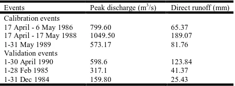
[image:3.612.64.296.450.535.2]Daily rainfall and stream-flow data for the period 1984-1990 was used in the study. The rainfall stations used were purposively selected within the study area, while only the river gauging station at the basin outlet was used. The analysis involved selecting sections with continuous data for both rainfall and streamflow. The selection was mainly dictated by the availability of streamflow data. These sections are referred herein as events. A total of six events each consisting of daily rainfall for all meteorological stations and corresponding daily discharges at the river gauging station (outlet) were identified as: 17 April – 6 May 1986; 17 April-17 May 1988; 1-31 May 1989; 1-31 Dec 1984; 1-28 Feb 1985 and 1-30 April 1990. The first three events were used for model calibration while the other three events were used for model validation. The main characteristics of each event are summarized in Table 2.
Table 2. Main characteristics of events
Events Peak discharge (m3
/s) Direct runoff (mm)
Calibration events
17 April - 6 May 1986 799.60 65.37
17 April - 17 May 1988 1049.50 189.07
1-31 May 1989 573.17 81.76
Validation events
1-30 April 1990 598.6 123.84
1-28 Feb 1985 317.1 41.37
1-31 Dec 1984 159.80 25.43
Curve number computation
The curve number (CN) is a function of hydrologic soil group, cover type, land use and antecedent moisture condition. In order to determine curve number, the land cover and soil type cover ages were combined through overlay analysis of GIS. The resulting coverage was used to delineate the sub-basin area into sub-areas that have same land use and soil type characteristics. The soils in the study area were broadly classified into hydrologic soil groups B and C. In this study, each sub-basin was assigned the dominant soil type and assumed uniform. The sub-basins with hydrologic soil group B were SBB3, SBB4, SBB5, SBB6 and SBB7 while those with hydrologic soil group C were SBB1, SBB2, SBB8 and SBB9. The curve number for every sub-area was obtained using appropriate tables such as those developed by SCS (1985). The representative curve number of each sub-basin was determined as the weighted average of all CN values of the sub-areas given by the expression:
) 1 .( ... ... ... ... ... ... ... ... ... ... 1 A A CN CN N i i i
where Ai and CNi are the area and the curve number of sub-area in
each sub-basin i, respectively. The moisture condition II was assumed during estimation of CN. The CN is one of the direct inputs in the hydrologic model. The land cover data from the classified Land sat Thematic image of 1988 was used to estimate the initial curve numbers required in the hydrologic model.
Calibration, Validation and Evaluation of HEC-HMS Model
The purpose of calibration was to obtain optimal values of curve numbers, initial discharges, recession constants, threshold discharges, and the Muskingum routing coefficients (K and x). The model calibration was performed using the optimization option available in HEC-HMS program version 3.5 (USACE, 2010). During the calibration process, initial values of curve numbers were computed using the 1988 land cover data, while arbitrary initial values of initial discharge, threshold discharge, recession constant, K and x were chosen. The calibration process involved adjusting the parameters until the observed and predicted hydrographs were close fit. The
modelvalidation involved predicting hydrographs using the optimal
parameters. The predicted hydrographs were then compared to the observed hydrographs recorded at outlet of the basin. In the study, main interest was the peak discharge and runoff depth measured at the outlet of the basin. The optimal parameters were used to evaluate model performances during calibration and validation. The coefficient of efficiency (COE) proposed by Nash and Sutcliffe (1970), mean
error (ME), percentage deviation of peak discharges (Dp) and
percentage deviation of discharges (Dv) were used to evaluate the
model performance. They are expressed as follows:
) 2 ....( ... ... ... ... ... ... ... ... ) ( ) ( 1 2 2
m oi ip oi q q q q COE ) 3 ....( ... ... ... ... ... ... ... ... ... ) ( n q qME
pi oi) 4 ( ... ... ... ... ... ... ... ... ... 100 ) ( op op pp p q Q q D ) 5 ...( ... ... ... ... ... ... ... ... 100 ) (
oi oi pi v q q q DWhere qpi is the predicted flow of day i (mm), qoi is the observed flow
of day i (mm), qm is the mean of all observed flows, qpp is the
predicted peak discharge (m3/s), qop is the observed peak discharge
(m3/s) at the basin outlet. In addition, the match was visually assessed
using the overall shape and fit of hydrographs. In addition, the product moment correlation coefficient (r) and coefficient of determination
(R2) were used to evaluate the model performance.
Predicting Impacts of Land Cover and Land Use Changes
Runoff depths, peak discharges and the general shapes of the hydrographs were used to quantify impact of land cover and use
changes. The events used in modelvalidation were later used in the
prediction of impact of land cover changes in the periods 1984-2010. The land cover and use data of 1984 and 2010 were used to compute the curve numbers required in the model. The impacts were quantified using the percentage changes in peak discharges and runoff depths recorded at the outlet of the study area.
RESULTS AND DISCUSSION
Land cover and use change detection
shown in Table 3. From Table 3 it is evident that agricultural and built-up lands increased between 1984 and 2010. The agricultural
land increased from 489.6 km2 (8.59%) in 1984 to 983.90 km2
(17.27%) in 2010, while built-up land increased from 1184.30 km2
(20.78%) in 1984 to 2534.60 km2 (44.48%) 2010. In the entire
period the agricultural land and built-up land increased by 494.20
km2 and 1350.30 km2, representing an increase of 8.67% and 23.70%
respectively. On the other hand, broadleaved evergreen forest, rangeland and closed/open woody vegetation decreased between 1984 and 2010. The broadleaved evergreen forest decreased from
260.50km2 (4.57%) to 117.00 km2 (2.05%). The rangelands
decreased from 2323.50 km2 (40.78%) to 1190.90 km2 (20.90%),
while closed/open woody vegetation decreased from 1439.60 km2
(25.27%) to 871.10 km2 (15.29%). Overall the broadleaved
evergreen forest, closed/open woody vegetation and rangelands
decreased by 143.50, 568.50 and 1132.60 km2, representing decrease
[image:4.612.305.545.66.454.2] [image:4.612.64.295.447.729.2]of 2.52%, 9.98 and “19.88%” respectively. The distribution of the different land cover types in 1984 and 2010 are shown in Figures 3 and 4, respectively. From Figures 3 and 4 it is evident that the agricultural land increased due to conversion of closed/open woody vegetation and broadleaved evergreen forest, while built-up land increased due to conversion of rangelands. The small decrease in broadleaved evergreen forest could be attributed to protection by Kenya Forest Service, since this category of land cover includes the Southern Abardare forest, which is a gazetted forest. On the other hand, increase in built-up land can be attributed to rural-urban migration.
Fig. 3. Land cover types as derived from Landsat TM of 1984
Fig. 4. Land cover types as derived from Landsat TM of 2010
Hydrological Modeling
Model Calibration, Validation and Evaluation
The optimal parameters obtained during calibration are shown in Tables 4 and 5 while the results of model evaluation are shown in Table 6 and illustrated graphically in Figures 5-10. From Table 5 it can be noted that the values of x were within the acceptable range of 0 - 0.5. The results of model performance evaluation using the optimal parameters during calibration and validation is given in Table 7 while Figures 5-10 show the predicted and observed flow hydrographs. The coefficient of efficiency (COE) between predicted and observed flow hydrographs were in the range 0.9308 to 0.9772 with mean COE of 0.9514 for the calibration events and COE in the range 0.8685 to 0.9529 with a mean COE of 0.9003 for validation events. The values of COE can be regarded as acceptable for all calibration and validation events, meaning a good fit between predicted and observed
values. These findings are in agreement to those of Chen et al. (2009)
Table 4. Optimal values of K and x
Reach K (hours) x
RCH1 35.31 0.22
RCH2 12.75 0.19
RCH3 4.6 0.19
RCH4 4.4 0.22
RCH5 5.99 0.20
Table 3. Land cover and land use in 1984, 1988 and 2010
Land cover type 1984 1988 2010 % Change
1984-2010
Area (km2
) % Area (km2
) % Area (km2
) %
Broadleaved evergreen forest
260.5 4.57 277.3 4.87 117.0 2.05 -2.05
Closed and open woody vegetation
1439.6 25.27 962.9 16.90 871.10 15.29 -9.98
Rangeland 2323.50 40.78 2038.40 35.61 1190.90 20.90 -19.88
Agricultural land 489.6 8.59 813.4 14.28 983.90 17.27 8.67
Built-up land 1184.3 20.78 1605.5 28.18 2534.60 44.48 23.70
[image:4.612.350.514.674.731.2]who obtained COE values ranging from 0.796 to 0.934 with an average of 0.885 during calibration and COE values ranging from 0.750 to 0.950 with a mean of 0.873 during validation of HEC-HMS model in Xitiaoxi basin, China and regarded the results as satisfactory. The mean errors (ME) were less than 10% except for one event (19.23%), indicating satisfactory performance overall. The percentage deviations of peak discharges and percent deviations of daily discharges were acceptable (less than 10%) except for one (-13.97%).
Chen et al. (2009) obtained percentage deviations in peak discharge
that were within 10% error and percent deviations in runoff volumes that were less than 10%, except for one event (10.9%) during calibration and recommended the use of the model. On the other hand,
Razi et al. (2010) observed 4% percent deviation in peak discharge in
[image:5.612.136.484.65.159.2]Johor River, Malaysia and recommended the use of the HEC-HMS model for estimating peak discharge. The results of the study have demonstrated that the calibrated and validated HEC-HMS model of the study area can be used for prediction of direct runoff and peak discharges satisfactorily. Figures 5-10 show the predicted and observed flow hydrographs.
Fig. 5. Predicted and observed flow using 17 April-6 May1986 event.
[image:5.612.299.548.78.409.2]Fig. 6. Predicted and observed flow hydrographs for 17April-17May 1988 event.
[image:5.612.316.551.428.560.2]Fig. 7. Predicted and observed flow hydrographs for 1-31May 1989 event.
Fig. 8. Predicted and observed flow hydrographs for 1-30April 1990 event.
Fig. 9. Predicted and observed flow hydrographs for 1-28 Feb 1985 event.
0 100 200 300 400 500 600 700 800 900
4/17/86 4/19/86 4/21/86 4/23/86 4/25/86 4/27/86 4/29/86 5/1/86 5/3/86 5/5/86
Days
fl
o
w
(
m
3/s
)
predicted flow observed flow
0 200 400 600 800 1000 1200 1400
4/12/1988 4/17/1988 4/22/1988 4/27/1988 5/2/1988 5/7/1988 5/12/1988 5/17/1988 5/22/1988
Days
F
lo
w
(
m
3/s
)
Predicted flow Observed flow
0 100 200 300 400 500 600 700
4/27/1989 5/2/1989 5/7/1989 5/12/1989 5/17/1989 5/22/1989 5/27/1989 6/1/1989 6/6/1989
Days
F
lo
w
(
m
3/s
)
predicted flow Obs erved flow
0 100 200 300 400 500 600 700
3/28/1990 4/2/1990 4/7/1990 4/12/1990 4/17/1990 4/22/1990 4/27/1990 5/2/1990
Days
F
lo
w
(
m
3/s
)
Predicted flow observed flow
0 50 100 150 200 250 300 350
1/28/1985 2/2/1985 2/7/1985 2/12/1985 2/17/1985 2/22/1985 2/27/1985 3/4/1985
Days
F
lo
w
(
m
3/s
)
Predicted flow Observed f low
Table 5. Optimal parameters for each sub-basin
Sub-catchment Optimal CN Recession constant Initial discharge (m3/s) Threshold discharge (m3/s)
SBB1 66 0.83 9.39 10.70
SBB2 64 0.83 2.96 3.95
SBB3 61 0.83 9.39 3.95
SBB4 52 0.83 2.96 3.95
SBB5 56 0.83 2.96 3.95
SBB6 55 0.83 2.96 3.95
SBB7 55 0.83 2.96 3.95
SBB8 65 0.83 4.42 3.78
SBB9 67 0.83 3.00 4.03
Table 6. Results of model performance evaluation using calibration and validation events
Events Sample size qop (m3/s) qpp (m3/s) Qo (mm) Qp (mm) Dp (%) Dv (%) COE ME
Calibration events
17April- 6 May 1986 20 799.60 814.0 65.37 69.38 1.80 8.96 0.9772 19.23
17 April -17May 1988 31 1049.50 1004.3 189.07 179.14 -4.31 -0.48 0.9463 -1.92
1-31 May 1989 31 573.17 596.44 81.76 87.54 4.06 0.52 0.9308 0.94
Validation events
1-30 April 1990 30 598.6 643.0 123.84 119.74 7.42 2.28 0.8685 6.25
1-28 Feb 1985 28 317.1 272.80 41.37 30.50 -13.97 1.17 0.8796 1.15
[image:5.612.65.295.466.616.2] [image:5.612.319.547.521.709.2]Fig. 10. Predicted and observed flow hydrographs for 1-31 Dec 1984 event.
It can be noted that the predicted and observed flow hydrographs matched well, implying that the model predicted flows satisfactorily.
Hydrological impacts of land cover changes
[image:6.612.314.555.48.174.2]The validation events were used to quantify the hydrological impacts of land cover changes between 1984 and 2010. The results are represented in Table 8 and illustrated in Figures 11-13, respectively.
Table 8. Impact of land cover and land use change between 1984 and 2010
Event 1984 2010 % Change
qpp
(m3/s)
Qp
(mm)
qpp
(m3/s)
Qp
(mm)
qpp Qp
1-28 Feb 85 565.10 58.58 618.50 64.35 9.45 9.85
1-30 April 90 736.90 182.73 768.00 195.26 4.22 6.86
1-31 Dec. 84 294.50 26.84 362.70 31.65 23.16 17.92
The peak discharges and runoff depths increased by 4-23% and 6-18% respectively, between 1984 and 2010. In the same period, built-up land and agricultural land increased by 8.67% and 23.70% respectively, while broadleaved evergreen forest, closed/open woody vegetation and rangelands decreased by 2.52%, 9.98 and 19.88% respectively. Increase in built-up land led to creation of impervious surfaces which decreased infiltration and increased surface runoff. Increase in agricultural land also led to less protection of soil against raindrop impact, since after harvesting and shortly after sowing, the plants do not cover the soil completely. Also depending on the type of crop being grown, croplands tend to have a percentage of bare ground even during the peak of growing season and may be completely bare prior to planting. The decrease in forest reduced evapotranspiration, depression storage and infiltration, leading to increase in surface runoff. In the study the increase in peak discharge and runoff depths can be attributed mainly to increase in built-up and agricultural lands. The results of the study agree with
those obtained by other authors (e.g. Costa et al., 2003; Mustafa et al.,
2005; Chen et al., 2009; Githui et al., 2009; Ahn et al., 2008;
[image:6.612.315.551.220.353.2]Santillan et al., 2010).
Fig. 11. Change in flow hydrographs between 1984 and 2010 for 1-31 Dec 84 event.
It can be noted that Peak discharge increased from 294.5 m3/s to
362.70 m3/s, between 1984 and 2010 for the 1-31 Dec event,
representing an increase of 23.16%.
Fig. 12. Change in flow hydrographs between 1984 and 2010 for 1-28 Feb 85 event.
The peak discharge increased from 565.1 m3/s to 618.5 m3/s while
time to peak decreased by one day for the 1-28 Feb 1985 event.
Fig. 13. Change of flow hydrographs between 1984 and 2010 for 1-30April event.
Peak discharge increased from 736.9 m3/s to 768 m3/s for the 1-30
April 1990, while time to peak decreased by one day, between 1984 and 2010. The decrease in time to peak implied that the study area responded more quickly to rainfall events and hence more prone to flooding. The predicted peak discharges can be used to design water storage reservoir that would capture the high flows during the rainy season.
Conclusions and Recommendations
The study involved quantification of land cover changes and their corresponding hydrological impacts using a validated and calibrated HEC-HMS model of the study area. Land cover change analysis revealed a general increase in agricultural and built-up lands and decrease in broadleaved evergreen forest, closed/open woody vegetation and rangelands. Evaluation of HEC-HMS model showed that it could be used as a tool to predict peak discharges and runoff depths in the study area. The study revealed that changes in land cover/use led to a general increase in runoff depths and peak discharges, associated mainly to increase in agricultural and built-up lands. The HEC-HMS model is recommended in decision support for watershed land use planning and management because it was found capable of generating quantitative data which could provide useful information for local administrations and decision makers to scientifically develop land use policies which would minimize negative environmental impacts induced by land cover and land use changes.
Acknowledgements
We wish to acknowledge the Kenya Meteorological Department for providing climatic data, Water Resources Management Authority (Machakos Headquarters) for providing streamflow data, Kenya Soil Survey for providing soil data, and Regional Center for Mapping and Development for providing Landsat TM images used in the study.
REFERENCES
Ahn, G, Merry, C.J. and Gordon, S.I. (2008) The effects of urbanization on the hydrologic regime of the Big Darby Creek
0 50 100 150 200
11/29/1984 12/4/1984 12/9/1984 12/14/1984 12/19/1984 12/24/1984 12/29/1984 1/3/1985
Days
F
lo
w
(
m
3/s
)
Predicted flow observed flow
0 50 100 150 200 250 300 350 400
11/29/1984 12/4/1984 12/9/1984 12/14/1984 12/19/1984 12/24/1984 12/29/1984 1/3/1985
Da ys
F
lo
w
(
m
3/s
)
1984 2010
0 100 200 300 400 500 600 700
1/28/85 2/2/85 2/7/85 2/12/85 2/17/85 2/22/85 2/27/85 3/4/85
Days
F
lo
w
(
m
3/s
)
1984 2010
0 200 400 600 800 1000
3/28/1990 4/2/1990 4/7/1990 4/12/1990 4/17/1990 4/22/1990 4/27/1990 5/2/1990
Days
F
lo
w
(
m
3/s
)
[image:6.612.59.299.287.344.2] [image:6.612.62.300.557.687.2]Watershed, Ohio. ASPRS 2008 Annual Conference, Portland, Oregon, April 28-May2, 2008
Anderson, J.R., Hardy, E.E., Roach, J.T. and Wittmer, R.E. (1976) A land use and land cover classification system for use of remote sensing data. US Geological Survey Professional Paper 964. Chen, Y., Xu, Y. and Yin, Y. (2009) Impacts of land use change
scenarios on storm-runoff generation in Xitiaoxi basin, China. Quaternary International 208 (2009):121–128, 2009 Elsevier Ltd and INQUA.
Costa, M.H., Botta, A. and Cardille, J. A. (2003) Effects of large-scale changes in land cover on the discharge of the Tocantins River,
Southeastern Amazonia. Journal of Hydrology, 283: 206-217.
Coutu, G.W. and Vega, C. (2007) Impacts of land use changes on runoff generation in the East Branch of the Brandywine Creek
watershed using a GIS-based hydrologic model. Middle States
Geographer, 40: 142-149.
Fu, B.J, Zhao, W.W, Chen, L.D, Liu, Z.F and Lu, Y.H (2005)
Eco-hydrological effects of landscape pattern change. Landscape
Ecol Eng (2005) 1: 25–32 DOI 10.1007/s11355-005-0001-5. Githui, F., Mutua, F. and Bauwens, W. (2009) Estimating the impacts
of land-cover change on runoff using the soil and water assessment tool (SWAT): Case study of Nzoia catchment,
Kenya, Hydrological Sciences Journal, 54:5, 899-908.
Hernandez, M., Miller, S.N., Goodrich, D.C., Goff, B.F., Kepner, W.G., Edmonds, C.M., and Jones, K.G. (2000) Modeling runoff response to land cover and rainfall spatial variability in
semi-arid watersheds. Environmental Monitoring and Assessment.
64:285-298.
Lambrechts, C., Woodley, B., Church, C. and Gachanja, M. (2003) Aerial survey of the destruction of the Abardare range forests. United Nations Environment Programme, Nairobi, Kenya. Mustafa, Y.M., Amin, M.S.M., Lee, T.S. and Shariff, A.R.M. (2005)
Evaluation of land development impact on a tropical watershed
hydrology using remote sensing and GIS. Journal of Spatial
Hydrology, 5(2): 16-30.
Muthukrishnan, S., Harbor, J., Lim, K.J. and Engel, B.A. (2006) Calibration of a simple rainfall-runoff model for long-term
hydrological impact evaluation. URISA Journal, Vol. 18, No.2
Nash, J.E. and Sutcliffe, J.V. (1970) River flow forecasting through
conceptual models, 1, A discussion of principles. J. Hydrol.,
10:282-290.
Razi, M.A.M, Ariffin, J., Tahir, W. and Arish, N.A.M. (2010) Flood estimation studies using hydrologic Modeling System (HEC-HMS) for Johor River, Malaysia: J. Appl. Sci. 10(11): 930-939. ISSN 1812-5654.
Rosso, R. and Rulli, M.C. (2002) An integrated simulation method for flash-flood risk assessment: Effects of changes in land use under
historical perspective. Hydrology and Earth Systems Sciences,
6(3), 285-294.
Santillan, J.R., Makinano, M.M. and Paringit, E.C. (2010) Integrating remote sensing, GIS and hydrologic models for predicting land cover change impacts on surface runoff and sediment yield in a critical watershed in Mindanao, Philippines, International Archives of the photogrammetry, Remote Sensing and Spatial Information Science, Vol. XXXVIII, Part 8, Kyoto Japan 2010. Shoemaker, L., Lahlou, M., Bryer, M., Kumar, D. and Kratt, K.
(1997) Compendium of tools for watershed assessment and TMDL development. U.S Environmental Protection Agency, EPA841-B-97-006.
Suwanwelarkamtorn, R. (1994) GIS and hydrologic modeling for the
management of small watersheds, International Journal of
Applied Earth Observation and Geoinformation (ITC) 1994, 343-348.
USACE (United States Army Corps of Engineers), (2003) Geospatial Hydrologic modeling Extension, HEC-GeoHMS User’s Manual, version 1.1. USACE: Davis, California.
USACE (United States Army Corps of Engineers), (2010) Hydrologic Modeling System - HEC-HMS: User’s Manual Version 3.5, USACE, Davis, CA, USA (2010).