Numerical Solution of Tenth Order Boundary Value
Problems by Petrov-Galerkin Method with Quintic
B-splines as Basis Functions and Sextic B-Splines as
Weight Functions
K. N. S. Kasi Viswanadham
Department of Mathematics National Institute of TechnologyWarangal – 506004, India
S. V. Kiranmayi Ch.
Department of Mathematics National Institute of TechnologyWarangal – 506004, India
ABSTRACT
In this paper, a finite element method involving Petrov-Galerkin method with quintic B-splines as basis functions and sextic B-splines as weight functions has been developed to solve a general tenth order boundary value problem with a particular case of boundary conditions. The basis functions are redefined into a new set of basis functions which vanish on the boundary where the Dirichlet, the Neumann, the second order derivative and the third order derivative type of boundary conditions are prescribed. The weight functions are also redefined into a new set of weight functions which in number match with the number of redefined basis functions. The proposed method was applied to solve several examples of tenth order linear and nonlinear boundary value problems. The obtained numerical results were found to be in good agreement with the exact solutions available in the literature.
Keywords
Basis functions, Tenth order boundary value problem, Quintic B-splines, Sextic B-splines, Petrov-Galerkin method, Weight functions.
1.
INTRODUCTION
Consider a general linear boundary value problem of tenth order
(10) (9) (8) (7)
0 1 2 3
(6) (5) (4)
4 5 6 7
8 9 10
( ) ( ) ( ) ( ) ( ) ( ) ( ) ( )
( ) ( ) ( ) ( ) ( ) ( ) ( ) ( )
( ) ( ) ( ) ( ) ( ) ( ) ( ) ,
p t u t p t u t p t u t p t u t
p t u t p t u t p t u t p t u t
p t u t p t u t p t u t b t c t d
(1)
subject to the boundary conditions
2 2 3 3
(4) (4)
4
0 0 1 1
4
( ) , ( ) , ( ) , ,
( ) , ( )
(
, ( ) , ( )
)
)
,
( , ( )
u c A u d C u c A u d C
u
u c A u d C u c A u
A
C
c u d C
d
(2)
where Ai, Ci, i=0,1,2,3,4 are finite real constants and pi(t),
i=0,1,2,…,10 and b(t) are all continuous functions defined on the interval [c, d].
The tenth-order boundary value problems are known to arise in the study of astrophysics, hydrodynamic and hydro magnetic stability [1]. A class of characteristic-value problems of high order (as higher as twenty four) is known to arise in hydrodynamic and hydro magnetic stability [1]. When an infinite horizontal layer of fluid is heated from below, with the supposition that a uniform magnetic field is also applied across the fluid in the same direction as gravity and the fluid is
subject to the action of rotation, instability sets in. When this instability sets in as ordinary convection, it is modelled by a tenth-order ordinary differential equation [1]. The existence and uniqueness of the solution for these types of problems have been discussed in Agarwal [2]. Finding the analytical solutions of such type of boundary value problems in general is not possible. Over the years, many researchers have worked on tenth-order boundary value problems by using different methods for numerical solutions. Twizell et al. [3] developed a finite difference technique for the solution of eighth, tenth and twelfth order boundary value problems. Siddiqi and Twizell[4], Siddiqi and Ghazala [5] presented the solution of a special case of linear tenth order boundary value problems by using tenth order and eleventh order spline functions respectively. Wazwaz[6] developed a modified Adomian decomposition method for the solution of tenth and twelfth order boundary value problems. Siddiqi and Ghazala [7] presented the solution of a special case of linear tenth order boundary value problems by using non-polynomial spline techniques. Erturk and Shaher[8] presented differential transform method for the solution of tenth order boundary value problems. Geng and Li [9], Abbasbandy and Shirzdi[10] presented the solution of a special case of tenth order boundary value problems by using variational iteration techniques. Kasi Viswanadham and Showri raju [11], Kasi Viswanadham and Sreenivasulu [12] developed a quintic B-spline collocation method, a quintic B-B-spline Galerkin method to solve a general tenth order boundary value problem respectively. Reddy [13] developed a Petrov Galerkin method with quintic B-splines as basis functions and septic B-splines as weight functions to solve a general tenth order boundary value problem. So far, tenth order boundary value problems have not been solved by using Petrov-Galerkin method with quintic B-splines as basis functions and sextic B-splines as weight functions. This motivated us to solve a tenth order boundary value problem by Petrov-Galerkin method with quintic B-splines as basis functions and sextic B-splines as weight functions.
specified boundary conditions. In Section 4, the procedure to solve the nodal parameters has been presented. In section 5, the proposed method is tested on several linear and nonlinear boundary value problems. The solution to a nonlinear problem has been obtained as the limit of a sequence of solutions of linear problems generated by the quasilinearization technique [14]. Finally, in the last section, the conclusions are presented.
2.
JUSTIFICATION FOR USING
PETROV-GALERKIN METHOD
In Finite Element Method (FEM) the approximate solution can be written as a linear combination of basis functions which constitute a basis for the approximation space under consideration. FEM involves variational methods like Rayleigh Ritz method, Galerkin method, Least Squares method, Petrov-Galerkin method and Collocation method etc. In Petrov-Galerkin method, the residual of approximation is made orthogonal to the weight functions. When we use Petrov-Galerkin method, a weak form of approximation solution for a given differential equation exists and is unique under appropriate conditions [15, 16] irrespective of properties of a given differential operator. Further, a weak solution also tends to a classical solution of given differential equation, provided sufficient attention is given to the boundary conditions [17]. That means the basis functions should vanish on the boundary where the Dirichlet type of boundary conditions are prescribed and also the number of weight functions should match with the number of basis functions. Hence in this paper we employed the use of Petrov-Galerkin method with quintic B-splines as basis functions and sextic B-splines as weight functions to approximate a solution of tenth order boundary value problem.3.
DESCRIPTION OF THE PROPOSED
METHOD
Definition of quintic B-splines and sextic B-splines: The quintic B-splines and sextic B-splines are defined in [18-20]. The existence of quintic spline interpolate s(t) to a function in a closed interval [c, d] for spaced knots (need not be evenly spaced) of a partition c = t0 < t1 <…< tn-1 < tn= d
is established by constructing it. The construction of s(t) is done with the help of the quintic B-splines. Introduce ten additional knots t-5, t-4, t-3, t-2, t-1, tn+1, tn+2, tn+3, tn+4 and tn+5 in such a way that
t-5<t-4<t-3<t-2<t-1<t0 and tn<tn+1<tn+2<tn+3<tn+4<tn+5. Now the quintic B-splines
B t s
i( ) '
are defined by5 3
3 3 3
(
)
,
[
,
]
( )
( )
0,
i r
i i r i
i r
t
t
t
t
t
B t
t
otherwise
where
5
5 ( ) ,
( )
0,
r r
r
r
t t if t t
t t
if t t
and
3
3
( )
(
)
i r r i
t
t t
where {B-2(t), B-1(t), B0(t), B1(t),…,Bn-1(t), Bn(t), Bn+1(t),
Bn+2(t)} forms a basis for the spaceS5( ) of quintic
polynomial splines. Schoenberg [20] has proved that quintic B-splines are the unique nonzero splines of smallest compact support with the knots at
t-5<t-4<t-3<t-2<t-1<t0<t1<…<tn-1<tn<tn+1<tn+2<tn+3<tn+4<tn+5.
In a similar analogue sextic B-splines Ti(t)'s are defined by
6 4
3 4 3
(
)
,
[
,
]
( )
( )
0,
i r
i i r i
i r
t
t
t
t
t
T t
t
otherwise
where
6
6 ( ) ,
( )
0,
r r
r
r
t t if t t
t t
if t t
and
4
3
( )
(
)
i r r i
t
t t
where {T-3(t), T-2(t), T-1(t), T0(t), T1(t),… ,Tn-1(t), Tn(t), Tn+1(t),
Tn+2(t)} forms a basis for the space
S
6( )
of sexticpolynomial splines with the introduction of two more additional knots t-6 and tn+6 to the already existing knots t-5 to
tn+5. Schoenberg [20] has proved that sextic B-splines are the
unique nonzero splines of smallest compact support with the knots at
t-6<t-5<t-4<t-3<t-2<t-1<t0<t1<…<tn-1<tn
<tn+1<tn+2<tn+3<tn+4<tn+5<tn+6. To solve the boundary value problem (1) subject to boundary conditions (2) by the Petrov-Galerkin method with quintic B-splines as basis functions and sextic B-B-splines as weight functions, we define the approximation for u(t) as
2
2
( ) ( )
n j j j
u t
B t
3)where αj’s are the nodal parameters to be determined and
Bj(t)’s are quintic B-spline basis functions. In Petrov-Galerkin
method, the basis functions should vanish on the boundary where the Dirichlet type of boundary conditions are specified. In the set of quintic B-splines {B-2(t), B-1(t), B0(t), B1(t),…,
Bn-1(t), Bn(t), Bn+1(t), Bn+2(t)}, the basis functions B-2(t), B-1(t), B0(t), B1(t), B2(t), Bn-2(t), Bn-1(t), Bn(t), Bn+1(t) and Bn+2(t) do not vanish at one of the boundary points. So, there is a necessity of redefining the basis functions into a new set of basis functions which vanish on the boundary where the Dirichlet type of boundary conditions are specified. When the chosen approximation satisfies the prescribed boundary conditions or most of the boundary conditions, it gives better approximation results. In view of this, the basis functions are redefined into a new set of basis functions which vanish on the boundary where the Dirichlet, the Neumann, the second order derivative and the third order derivative type of boundary conditions are prescribed. The procedure for redefining of the basis functions is as follows.
Using the definition of quintic B-splines, the Dirichlet, the Neumann, the second order derivative and the third order derivative boundary conditions of (2), we get the approximate solution at the boundary points as
2
0 0 0
2
( ) ( ) j j( )
j
A u c u t
B t
(4)2
0
2
( ) ( ) ( )
n
n j j n
j n
C u d u t
B t
(5)2
1 0 0
2
( )
( )
j j( )
j
A
u c
u t
B t
2
1
2
( ) ( ) ( )
n
n j j n
j n
C u d u t
B t
(7)2
2 0 0
2
( ) ( ) j j( )
j
A u c u t
B t
(8)2
2
2
( ) ( ) ( )
n
n j j n
j n
C u d u t
B t
(9)2
3 0 0
2
( )
( )
j j( )
j
A
u
c
u
t
B
t
(10)2
3
2
( ) ( ) ( )
n
n j j n
j n
C u d u t
B t
(11)Eliminating α-2, α-1, α0, α1, αn-1, αn, αn+1 and αn+2 from the equations (3) to (11), we get
2 2 ( ) ( ) ( ) n j j j
u t w t
S t
(12)where
3
3 3 0 2 3
1
1 0 1
1 ( ) ( ) ( ) ) ( ) ( ( ) ) ) ( ( n n n n A C
w t w t R t R
R t R t
w t w t
t (13) 3 2
2 2 0 2 2
0 0 0 ( ) ( ) ( ) ) ( ) ( ( ( ) ) ) ( n n n n A C
w t w t Q t Q
t Q t
w t w t
t Q
(14)
2 1 1 1
1 1
1
1 0 1 1
0
( )
( )
( )
)
( )
(
( )
)
(
)
(
n n n nA
C
w t
w t
P t
P
t
w
t
w t
t
t
P
P
(15) 0 01 2 2
2 0 2
( ) ( ) ( )
( ) n ( )n n
A C
w t B t B t
B t B t
(16)
0 1 1 0 1 1 ( )
( ) ( ) , 2
( )
( ) ( ) , 3, 4,..., 3
( )
( ) ( ) , 2
( ) j j j j j n j n n n R t
R t R t j
R t
S t R t j n
R t
R t R t j n
R t
(17) 0 0 0 0
( )
( )
( ) ,
1, 2
( )
( )
( ) ,
3, 4,...,
3
( )
( )
( ) ,
2,
1
( )
j j j j j n j n n nQ t
Q t
Q t
j
Q t
R t
Q t
j
n
Q t
Q t
Q t
j
n
n
Q t
(18) 0 1 1 0 1 1( )
( )
( ) ,
0,1, 2
( )
( )
( ) ,
3, 4,...,
3
( )
( )
( ) ,
2,
1,
( )
j j j j j n j n n nP t
P t
P t
j
P t
Q t
P t
j
n
P t
P t
P
t
j
n
n
n
P
t
(19) 0 2 2 0 2 2( )
( )
( ) ,
1, 0,1, 2
( )
( )
( ) ,
3, 4,...,
3
( )
( )
( ) ,
2,
1, ,
1
( )
j j j j j n j n n nB t
B t
B
t
j
B
t
P t
B t
j
n
B t
B t
B
t
j
n
n
n n
B
t
(20) The new set of basis functions in the approximation u(t) is {Sj(t), j=2,3,…,n-2}. Here w(t) takes care of given set ofDirichlet, Neumann, the second and the third order derivative type of boundary conditions and Sj(t)'s and its first, the second
and the third order derivatives vanish on the boundary. In Petrov-Galerkin method, the number of basis functions in the approximation should match with the number of weight functions. Here the number of basis functions in the approximation for u(t) defined in (12) is n-3, where as the number of weight functions is n+6. So, there is a need to redefine the weight functions into a new set of weight functions which in number match with the number of basis functions. The procedure for redefining the weight functions is as follows:
Let us write the approximation for v(t) as 2 3 ( ) ( ) n j j j
v t T t
(21)where Tj(t)'s are sextic B-splines and here we assume that
above approximation v(t) satisfies the conditions
4
( ) 0, ( ) 0, ( ) 0, ( ) 0, ( ) 0, ( ) 0, ( ) 0, ( ) 0, ( ) 0.
v c v d v c v d v c
v d v c v d v c
(22)
Applying the boundary conditions (22) to (21), we get the approximate solution at the boundary points as
2
0 0
3
( )
( )
j j( )
0
j
v c
v t
T t
(23)2
3
( )
( )
( )
0
n
n j j n j n
v d
v t
T t
(24)2
0 0
3
( )
( )
j j( )
0
j
v c
v t
T t
(25)2
3
( )
( )
( )
0
n
n j j n j n
v d
v t
T t
(26)2
0 0
3
( )
( )
j j( )
0
j
v c
v t
T
t
(27)2
3
( )
( )
( )
0
n
n j j n j n
v d
v t
T
t
(28)2
0 0
3
( )
( )
j j( )
0
j
v
c
v
t
T
t
2
3
( )
( )
( )
0
n
n j j n j n
v
d
v
t
T
t
(30) 2
4 4 4
0 0
3
( )
( )
j j( )
0
j
v
c
v
t
T
t
(31)Eliminating β-3, β-2, β-1, β0, β1, βn-1, βn, βn+1 and βn+2 from the equations (21) and (23) to (31), we get the approximation for v(t) as 2 2 ˆ ( ) ( ) n j j j
v t
V t
(32)where 4 0 1 4 1 0
( )
( )
( ), j =2
ˆ ( )
( )
( ) ,
3, 4,...,
2.
j j
j
j
V
t
V t
V t
V t
V
t
V t
j
n
(33) 0 0 0 0 1 1( )
( )
( ) ,
1, 2
( )
( )
( ) ,
3, 4,...,
4
( )
( )
( ) ,
3,
2.
( )
j j j j n j n n nW
t
W t
W t
j
W
t
V t
W t
j
n
W
t
W t
W
t
j
n
n
W
t
(34) 0 1 1 0( )
( )
( ) ,
0,1, 2
( )
( )
( ) ,
3, 4,...,
4
( )
( )
( ) ,
3,
2,
1.
( )
j j j j j n j n n nV
t
V t
V
t
j
V
t
W t
V t
j
n
V
t
V t
V t
j
n
n
n
V
t
(35) 0 2 2 0 1 1( )
( )
( ) ,
1, 0,1, 2
( )
( )
( ) ,
3, 4,...,
4
( )
( )
( ) ,
3,
2,
1, .
( )
j j j j j n j n n nU t
U t
U
t
j
U
t
V t
U t
j
n
U t
U t
U
t
j
n
n
n
n
U
t
(36) 0 3 3 0 2 2( )
( )
( ),
2, 1, 0,1, 2
( )
( )
( ) ,
3, 4...,
4
( )
( )
( ),
3,
2,
1, ,
1.
( )
j j j j j n j n n nT t
T t
T
t
j
T
t
U t
T t
j
n
T t
T t
T
t
j
n
n
n
n n
T
t
(37) Now the new set of weight functions for the approximation v(t) is {V tˆ ( )j , j=2, 3,…,n-2}. Here V tˆ ( )j 's and its first, second and third order derivatives vanish on the boundary. Also fourth derivative of V tˆ ( )j ’s at left boundary also vanish.Applying the Petrov-Galerkin method to (1) with the new set of basis functions {Sj(t), j=2,3,…,n-2} and with the new set of
weight functions {V tˆ ( )j , j=2,3,…,n-2}, we get
0
0
(10) (9) (8) (7)
4 0
(6) (5)
5 6 7
8 9 10
1 2 3
4 ( ) ( ) ( ) ( ) ( ) ( ) ( ) ( ) ( ) ( ) ( ) ( ) ( ) ( ) ( ) ( ) ˆ ˆ ( ) ( ) ( ) ( ) ( ) ( )] ( ) ( ) ( ) [ n n t t t i t i
p t u t p t u t p t u t p t u t
p t u t p t u t p t u t p t u t
p t u t p t u t p t u t V t dt b t V t dt
for i 2, 3, , n-2.
(38)
Integrating by parts the first six terms on the left hand side of (38) and after applying the boundary conditions prescribed in (2), we get
0 0 0 5 5 5 4 4 5 5 6 6 4 (10)0 4 0
0 0 (4) 0 ˆ ˆ ( ) ( ) ( ) ( ) ( ) ˆ ˆ ( ) ( ) ( ) ( ) ˆ ( ) ( ) ( )
[
]
[
]
[
]
[
]
n n n n t t n t t t t t i i i i i dt u t V t dt t V t
dt
d d
t V t t V
p p u t
p C p t
dt dt
d
t V t u
t
A
t
p t d
d
(39) 0 0 4 (9) 41 1 4
3 3 (4) 1
ˆ
ˆ
( )
( ) ( )
( ) ( )
ˆ
( ) ( )
( )
[
]
[
]
n n n i t t t i i t td
t u
t V t dt
t V t
p
p
C
p
dt
d
t V t
u
t dt
dt
(40) 0 0 4 4 ( 2 4 8) 2ˆ
ˆ
( )
( ) ( )
[
( ) ( )
]
( )
n n t t t i t id
t u
t V t dt
t V t
u
t dt
d
p
p
t
(41)0 0
4
3 4 3
(7)
ˆ
ˆ
( )
( ) ( )
[
( ) ( )
]
( )
n n t t t t i id
t u
t V t dt
t V t
u
t dt
dt
p
p
(42)0 0
(6)
4 4
4
( )
( ) ( )
ˆ
[
4( ) ( )
ˆ
]
( )
n n
t t
t t
i i
d
t u
t V t dt
t V t
u t dt
dt
p
p
(43)0 0
4
5 4 5
(5)
ˆ
ˆ
( )
( ) ( )
[
( ) ( )
]
( )
n n i i t t t td
t u
t V t dt
t V t
u t dt
d
p
p
t
(44)Substituting (39) to (44) in (38) and using the approximation for u(t) given in (12), and after rearranging the terms for resulting equations, we get a system of equations in the matrix form as
A
B
(45) where[
a
ij];
06 3
0 1
6 3
4
(4)
2 6
4 4
3 7
4 4
4 8
4 4
5 4
ˆ
ˆ
[
( )
( )
( )
( )
ˆ
ˆ
( )
( )
( )
( )]
( )
ˆ
ˆ
[
( )
( )
( )
( )]
( )
ˆ
ˆ
[
( )
( )
( )
( )]
( )
ˆ
[
( )
( )
n
t
ij i i
t
i i j
i i j
i i j
i
d
d
a
p t V t
p t V t
dt
dt
d
p t V t
p t V t S
t
dt
d
p t V t
p t V t S
t
dt
d
p t V t
p t V t S
t
dt
d
p t V t
dt
9
4
5
10 4 0
ˆ
( )
( )]
( )
ˆ
ˆ
( )
( )
( )
( )
( )
( )
n
i j
i j i j n
t
p t V t S
t
d
p
t V t S
t
dt
p t V t
S
t
dt
for i= 2, 3,…, n-2; j= 2,3,…, n-2. (46)
[ ];
b
i
B
0
6 3
0 1
6 3
4 4
4
2 6 3
4 4
4
7 4 4 8
4 5 4
ˆ ˆ ˆ
{ ( ) ( ) {[ ( ) ( ) ( ) ( )
ˆ ˆ ˆ
( ) ( ) ( ) ( )] ( ) [ ( ) ( )
ˆ ˆ ˆ
( ) ( )] ( ) [ ( ) ( ) ( ) ( )] ( )
ˆ
[ ( )
n
t
i t i i i
i i i
i i i
i
d d
b b t V t p t V t p t V t
dt dt
d d
p t V t p t V t w t p t V t
dt dt
d
p t V t w t p t V t p t V t w t
dt d
p t V dt
0
9 10
5 5
0 4 0 4
5 5
4 4
5
1 4 0
4 4
ˆ ˆ
( ) ( ) ( )] ( ) ( ) ( ) ( )}}
ˆ ˆ
( ) ( ) ( ) ( )
ˆ ˆ
( ) ( ) ( ) ( ) ( )
n
n n
i i
i i
t t
i i n
t t
t p t V t w t p t V t w t dt
d d
p t V t C p t V t A
dt dt
d d
p t V t C p t V t w t
dt dt
for i=2, 3, ..., n-2. (47)
and
[
2 3
n2]
T.
4.
PROCEDURE OF SOLVING THE
NODAL PARAMETERS
A typical integral element in the matrix A is1
0
n m m
I
where1
( ) ( ) ( )
m
m
t j t
m i
I
v
t
r t Z t dt
,r t
j( )
are the quintic B-splinebasis functions or their derivatives,
v t
i( )
are the sexticB-spline weight functions or their derivatives. It may be noted that Im = 0 if (ti3,ti4)(tj3,tj3)( ,t tm m1) . To evaluate eachIm, we employed 7-point Gauss-Legendre quadrature formula. Thus the stiffness matrix A is a twelve diagonal band matrix. The nodal parameter vector has been obtained from the system
A
B
using the band matrix solution package. We have used the FORTRAN-90 program to solve the boundary value problems (1) - (2) by the proposed method.5.
NUMERICAL RESULTS
To demonstrate the applicability of the proposed method for solving the tenth order boundary value problems of the type (1) and (2), we considered three linear and three nonlinear boundary value problems. The obtained numerical results for each problem are presented in tabular forms and compared with the exact solutions available in the literature.
Example 1: Consider the linear boundary value problem 3
(10)
(80 19
)
t,
0
1
u
tu
t
t
e
t
(48)subject to
(4) (4)
(0) 0, (1) 0, (0) 1, (1) ,
(0) 0, (1) 4 , (0) 3, (1) 9 ,
(0) 8, (1) 16 .
u u e
e u e
u u
u u u
u u e
The exact solution for the above problem is
(1
) .
tu
t
t e
[image:5.595.52.276.65.578.2]The proposed method is tested on this problem where the domain [0, 1] is divided into 10 equal subintervals. The obtained numerical results for this problem are given in Table 1. The maximum absolute error obtained by the proposed method is 8.905812x10⁻⁶.
Table 1: Numerical results for Example 1 t Absolute error by the
proposed method
0.1 9.020966E-07
0.2 5.777913E-06
0.3 8.905812E-06
0.4 8.701042E-06
0.5 7.126059E-06
0.6 5.418603E-06
0.7 3.075147E-06
0.8 1.373522E-06
0.9 1.987132E-07
Example 2: Consider the linear boundary value problem 2
(10) 2
10cos
( 2) t (t 1) ( 1)sin , 1 1
u t u t t t
(49) subject to
(4) (4)
( 1) 2sin1, (1) 0,
( 1) 2 cos1 sin1, (1) sin1,
( 1) 2 cos1 2sin1, (1) 2 cos1,
( 1) 2 cos1 3sin1, (1) 3sin1,
( 1) 4 cos1 2sin1, (1) 4 cos1.
u u
u u
u u u
u
u u
The exact solution for the above problem is
u
(
t
1)sin .
t
Table 2: Numerical results for Example 2 t Absolute error by the
proposed method
-0.8 1.877546E-07
-0.6 1.830607E-06
-0.4 3.629923E-06
-0.2 4.529579E-06
0.0 3.836668E-06
0.2 1.795404E-06
0.4 8.996576E-08
0.6 5.906447E-07
0.8 4.263596E-07
Example 3: Consider the linear boundary value problem
(10) (9) (4) 2
2
sin
cos
(2 sin
cos
) ,
t0
1
u
t u
t u
t u
t
t
t e
t
u
(50)subject to
(4) (4)
(0) 1, u(1) , (0) 1, (1) ,
(0) 1, (1) , (0) 1, (1) ,
(0) 1, (1) .
u e e
u e e
u
e u
u u u
u u
The exact solution for the above problem is
u
e
t.
[image:6.595.362.497.333.505.2]The proposed method is tested on this problem where the domain [0, 1] is divided into 10 equal subintervals. The obtained numerical results for this problem are given in Table 3. The maximum absolute error obtained by the proposed method is 5.668445x10⁻⁶.
Table 3: Numerical results for Example 3 t Absolute error by the
proposed method
0.1 1.818752E-07
0.2 1.007892E-06
0.3 2.970629E-06
0.4 5.213757E-06
0.5 5.668445E-06
0.6 3.796645E-06
0.7 1.136720E-06
0.8 4.546880E-07
0.9 6.214070E-07
Example 4: Consider the nonlinear boundary value problem
(10) 2 3
,
0
1
t t
t
u
e u
e
e
t
(51)subject to
The exact solution for the above problem is
u
e
t.
The nonlinear boundary value problem (51) is converted into a sequence of linear boundary value problems generated by quasilinearization technique [14] as
(10) 2
( 1) ( ( )
( 1 )
3
)
2
,
0,1, 2,...
t t t
n
t
n n
n
u
e
u
u
e
e
e
n
u
(52)
subject to
1 1
( 1) ( 1) ( 1) ( 1)
1 1
( 1) ( 1) ( 1) ( 1)
(4) (4) 1
( 1) ( 1)
(0) 1, (1) , (0) 1, (1) ,
(0) 1, (1) , (0) 1, (1) ,
(0) 1, (1) .
n n n n
n n n n
n n
u e u u e
u u e u u e
u u
u
e
Here
u
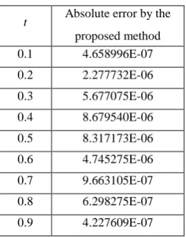
(n1) is the(n1)th approximation for u(t). The domain [0, 1] is divided into 10 equal subintervals and the proposed method is applied to the sequence of linear problems (52). The obtained numerical results for this problem are presented in Table 4. The maximum absolute error obtained by the proposed method is 8.679540x10⁻⁶.Table 4: Numerical results for Example 4 t Absolute error by the
proposed method
0.1 4.658996E-07
0.2 2.277732E-06
0.3 5.677075E-06
0.4 8.679540E-06
0.5 8.317173E-06
0.6 4.745275E-06
0.7 9.663105E-07
0.8 6.298275E-07
0.9 4.227609E-07
Example 5: Consider the nonlinear boundary value problem
(10)
14175
11(
1) ,
0
1
4
t
u
t
u
(53)subject to
(4) (4)
(0)
0, (1)
0,
(0)
0.5,
(1)
1,
(0)
0.5,
(1)
4,
(0)
0.75,
(1)
12,
(0)
1.5,
(1)
48.
u
u
u
u
u
u
u
u
u
u
The exact solution for the above problem is 2 1. 2
u t
t
The nonlinear boundary value problem (53) is converted into a sequence of linear boundary value problems generated by quasilinearization technique [14] as
10 (10)
( 1) ( 1)
10
155925
1 4
1
, 0,1, 2,
4175
..
1 1 10
4 .
n
n n
n n
t u u
t t
u
u n
u
1 1
1 1
(4) (4) 1
(0)
1, (1)
,
(0)
1,
(1)
,
(0)
1,
(1)
,
(0)
1,
(1)
,
(0)
1,
(1)
.
u
u
e
u
u
u
u
u
u
u
e
u
e
e
e
[image:6.595.96.238.479.654.2](54) subject to
( 1) ( 1) ( 1) ( 1)
( 1) ( 1) ( 1) ( 1)
(4) (4)
( 1) ( 1)
(0)
0,
(1)
0,
(0)
0.5,
(1)
1,
(0)
0.5,
(1)
4,
(0)
0.75,
(1)
12,
(0)
1.5,
(1)
48.
n n n n
n n n n
n n
u
u
u
u
u
u
u
u
u
u
[image:7.595.96.238.245.418.2]Here
u
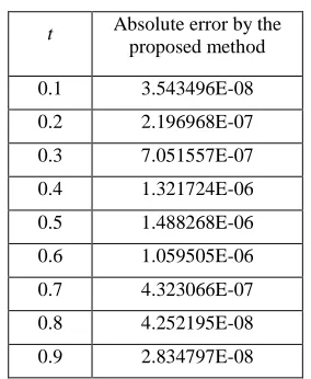
(n1) is the(n1)th approximation for u(t). The domain [0, 1] is divided into 10 equal subintervals and the proposed method is applied to the sequence of linear problems (54). The obtained numerical results for this problem are presented in Table 5. The maximum absolute error obtained by the proposed method is 1.488268x10⁻⁶.Table 5: Numerical results for Example 5 t Absolute error by the
proposed method
0.1 3.543496E-08
0.2 2.196968E-07
0.3 7.051557E-07
0.4 1.321724E-06
0.5 1.488268E-06
0.6 1.059505E-06
0.7 4.323066E-07
0.8 4.252195E-08
0.9 2.834797E-08
Example 6: Consider the nonlinear boundary value problem
9 2 4
(10) 2
cos
(2
cos( )) ,
0
1
t t t
u
u
u u
t
u
e
u
e
e
(55)subject to
(4) (4)
(0) 1, (1) , (0) 1, (1) , (0) 1,
(1) , (0) 1, (1) , (0) 1, (1) .
u u u
u u u u
u u e e
u e e e
The exact solution for the above problem is
u
e
tThe nonlinear boundary value problem (55) is converted into a sequence of linear boundary value problems generated by quasilinearization technique [14] as
9 2 4
(10)
1 1
4
1
4
1 1
2
cos
2 sin
2 sin 2 c
os
0,1 2, ,. ..
n n
n
n n n
n
t n
n n
n
n
t t
n n n
n
u u u u u u
u u u u
u u u u e e e
n u
u
(56) subject to
( 1) ( 1) ( 1) ( 1)
( 1) ( 1) ( 1) ( 1)
(4) (4)
( 1) ( 1)
(0)
1,
(1)
,
(0)
1,
(1)
,
(0)
1,
(1)
,
(0)
1,
(1)
,
(0)
1,
(1)
.
n n n n
n n n n
n n
u
u
e u
u
e
u
u
e u
u
e
u
u
e
Here
u
(n1) is the(n1)th approximation foru t
( ).
The domain [0, 1] is divided into 10 equal subintervals and the proposed method is applied to the sequence of linear problems (56). The obtained numerical results for this problem are presented in Table 6. The maximum absolute error obtained by the proposed method is 7.127641x10⁻⁶.Table 6: Numerical results for Example 6 t Absolute error by the
proposed method
0.1 2.520382E-07
0.2 1.350924E-06
0.3 3.871307E-06
0.4 6.684054E-06
0.5 7.127641E-06
0.6 4.597178E-06
0.7 1.209783E-06
0.8 6.855440E-07
0.9 8.266854E-07
6.
CONCLUSION
In this paper, we have employed a Petrov-Galerkin method with quintic B-splines as basis functions and sextic B-splines as weight functions to solve a general tenth order boundary value problem with special case of boundary conditions. The quintic B-spline basis set has been redefined into a new set of basis functions which vanish on the boundary where the Dirichlet, the Neumann, the second order derivative and the third order derivative type of boundary conditions are prescribed. The sextic B-splines are redefined into a new set of weight functions which in number match the number of redefined set of basis functions. The solution to a nonlinear problem has been obtained as the limit of a sequence of solution of linear problems generated by the quasilinearization technique [14]. The proposed method has been tested on three linear and three nonlinear tenth order boundary value problems. The numerical results obtained by the proposed method are in good agreement with the exact solutions available in the literature. The strength of the proposed method lies in its easy applicability, accurate and efficient to solve tenth order boundary value problems.
7.
REFERENCES
[1] S.Chandrasekhar, 1981, Hydrodynamic and Hydromagmetic Stability, Dover, New York.
[2] R.P. Agarwal, 1986, Boundary Value Problems for Higher Order Differential Equations, World Scientific, Singapore.
[3] E.H.Twizell, A.Boutayeb and K.Djidjeli, Numerical methods eighth,tenth and twelfth order eigen value problems arising in thermal instability, Advances in Computational Mathematics, vol.2 (1994), pp.407-436. [4] Shahid S.Siddiqi and E.H.Twizell, Spline solutions of
linear tenth-order boundary value problems, International Journal of Computer Mathematics, vol. 68 (1998), pp.345-362.
spline, Applied Mathematics and Computation, vol. 185 (2007), pp.115-127.
[6] Abdul-Majid Wazwaz, The modified Adomain decomposition method for solving linear and nonlinear boundary value problems of tenth and twelfth order, International Journal of Nonlinear Sciences and Numerical Simulation, vol. 1 (2007), pp.115-127. [7] Shahid S.Siddiqui and Ghazala Akram, Solution of tenth
order boundary value problems using non-polynomial spline technique, vol. 190 (2007), pp.641-651.
[8] Vedat Suat Erturk and Shaher Momani, A reliable algorithm for solving tenth order boundary value problems, Numerical Algorithms, vol. 44 (2007), pp.147-158.
[9] Fazhan Geng and Xiuying Li, “Variational iteration method for solving linear tenth order boundary value problems, Mathematical Sciences, vol.3 (2009), pp.161-172.
[10]A.Abbasbandy and A.Shirzadi, The variational iteration method for a class of tenth order boundary value problems, International Journal of Industrial Mathematics, vol.2 (2010), pp.29-36
[11]K.N.S.Kasi Viswanadham and Y.Showri Raju, Quintic B-spline collocation method for tenth order boundary value problems, International Journal of Computer Applications, vol. 51 (2012), pp.7-13.
[12]K.N.S.Kasi Viswanadham and Ballem Sreenivasulu, Numerical solution of tenth order boundary value
problems by Galerkin method with quintic B-splines, International Journal of Applied Mathematics and Statistical Sciences, vol. 3 (2014), pp.17-30.
[13]S.M.Reddy, Numerical solution of tenth order boundary value problems by Petrov Galerkin method with quintic B-splines as basis functions and septic B-splines as weight functions, International Journal of Engineering and Computer Science, vol. 5 (2016), pp.17894-17901. [14]R.E.Bellman and R.E. Kalaba, 1965, Quasilinearzation
and Nonlinear Boundary Value Problems, American Elsevier, New York.
[15]L.Bers, F.John and M.Schecheter, 1964, Partial Differential Equations, John Wiley Inter science, New York.
[16]J.L.Lions and E.Magenes, 1972, Non-Homogeneous Boundary Value Problem and Applications. Springer-Verlag, Berlin.
[17] A.R.Mitchel and R.wait, 1997, The Finite Element Method in Partial Differential Equations, John Wiley and Sons, London.
[18]P.M. Prenter, 1989, Splines and Variational Methods, John-Wiley and Sons, New York.
[19]Carl de-Boor, 1978, A Pratical Guide to Splines, Springer-Verlag