Towards Solving Travelling Salesperson Problem using Hybrid of Genetic Algorithm and Lin Kernighan Algorithm: A Comparative Evaluation with Neural Network Model

11

Towards Solving Travelling Salesperson Problem using

Hybrid of Genetic Algorithm and Lin-Kernighan

Algorithm: A Comparative Evaluation with Neural

Network Model

Samuel A. Oluwadare

Computer Science Department

Federal University of

Technology Akure, Nigeria

Bosede A. Ogunsanmi

Computer Science Department

Federal University of

Technology Akure, Nigeria.

John C. Nwaiwu

Computer Science Department

Federal University of

Technology Akure, Nigeria

ABSTRACT

Travelling salesperson problem involves the sales person who intends to find the minimum or shortest round trip that passes through a finite set of cities, exactly once at minimum cost. This problem belongs to the class of optimization problems which is described as non-deterministic polynomial hard, that is, it cannot be solved in exact polynomial time. Several approaches have been employed in solving the problem, but empirical results has shown that these approaches needs more optimization in terms of run time and quality of getting the optimum solution. Genetic algorithm combined with another local search algorithm shows more efficient result could be obtained. In this paper, hybridization of genetic algorithm with a local search algorithm called Lin-Kernighan algorithm is employed to provide efficient solution. A case study of finding the optimal solution for a tour of state capitals in Southern Nigeria is carried out. The model is implemented on Intel Celeron 2GHz, 1GB RAM machine with JAVA programming language and Wamp sever. The performance of the proposed hybrid genetic algorithm-based model is compared with Artificial Neural Network. The results showed that the proposed model performs better than neural network in terms of run-time and minimal tour distance.

General Terms

Routing, Optimization, Genetic Algorithm

Keywords

Travelling salesperson problem, Genetic algorithm, Lin-Kernighan algorithm, Neural network, Optimal solution

1.

INTRODUCTION

Travelling salesman problem (TSP) is well known non-deterministic polynomial-time (NP-Hard) problem in combinatorial optimization which requires the shortest path through a tour through n cities, passing each once and returns to the first visit. An NP-hard problem is the one that cannot be solved exactly in polynomial time, that is, it does not have an exact but approximate solution. TSP research finds its application in different areas such as transportation problem, logistic distribution problem, delivery order problem, minimum spanning tree (MST) for communication network, electricity network or water pipelining, and machine flow shop scheduling [1]. Another variant of TSP is the Dynamic traveling salesman problem (DTSP), which is a modified version of the travelling salesman [2,3]. Here, a salesman embarks on a trip starting from a city and after a complete round comes back to his starting point whilst passing each city once. Addition or removal of cities is allowed in DTSP [4].

This research dwells on standard TSP. The idea of TSP problem is to find the shortest path of tour starting from a given city, passing once an n city and returning back to the city of take off. The major research problem lies in what order should a traveling salesman tour the cities in order to achieve an optimal minimum distance? In view of achieving TSP solution had led to emergence of two categories of algorithms namely, exact and approximate algorithms. The exact algorithm has high computational time while approximate method, based on heuristics, is more suitable. These set of algorithms had found solutions in TSP [6, 7, 8, 9, 10].

For larger TSP, it is computationally costly to obtain optimal solution using exact algorithms, thus the context for the development and application of approximate algorithms or heuristics is investigated in this paper. The study of algorithms to achieve this practical goal has been carried out by applying different methods from many areas such as heuristic methods [12], simulated annealing [30], tabu search, ant colony [13], [14], [15], particle swam optimization [16], [17], fuzzy and neural network [18], [19]. However, it is obvious that these techniques are grossly inefficient and impracticable because of vast number of possible solutions to the TSP, hence leading to the exploration of the advantages of hybrid genetic algorithm and heuristics.

12 compared with local search based algorithms. This can be

attributed to the computational cost accrued to population based search in GAs. However, the major reason arises from the fact that crossover operators require more computational cost to generate an offspring solution than do local search operators to evaluate a solution in the neighbourhood [22]. A local search algorithm‟s ability to locate local optima with high accuracy complements the ability of genetic algorithms to capture a global view of the search space [23].

This paper presents a hybrid genetic algorithm-based model that provides an optimal solution to the travelling salesperson problem. The model incorporate Lin-Kernighan algorithm into mutation process of the genetic algorithm to produce a more efficient solution to the travelling salesperson problem. The remainder of this paper is organized as follows. Section 2 provides a detailed literature review on travelling salesman problem and hybrid genetic algorithm models. A proposed hybrid genetic and Lin-Kernighan algorithm model is presented in Section 3 while Section 4 shows the implementation results and evaluation with neural network model. The paper concludes in section 5 with notable findings and future areas of research.

2.

LITERATURE REVIEW

2.1

Traveling Salesman Problem

The travelling salesperson problem (TSP) is shown [5] with full graph with weighted edges;

 

V E

G , (1)

that V is a set of n node or vertex (n = |V|) that indicates cities and E ⊆ V ×V is a set of edges or directed edges. To each edge (i, j) ∈ E the length of djj that is the distance between the cities of I and j that is i, j ∈ V, is attributed. The travelling salesperson problem can be naturally Symmetric or asymmetric [11]. In the asymmetric travelling salesperson problem (ATSP), the distance between the nodes of i and j is dependent on edge scan direction, at least one edge (i, j) that there is dij ≠ dji. In the symmetric travelling salesperson problem, for all of the edges dij is equal to dji in E. The solution of the travelling salesperson problem is to find Hamiltonian cycle with the least length of graph. Hamiltonian cycle is a traversal of a path in an undirected or directed graph through its vertex exactly once. Such a graph is a traceable graph. A combination of v vertices starting from {1,…,v} such that the total length is a function of v is of minimal cost, gives the optimal solution for solving traveling salesman problem.

The adopted mathematical model for travelling salesperson problem is as follows [24]:



 n j i j i j i

x

d

Min

1 , ,

, (2)

Subject to the constraints:









n j j

i

i

n

x

1

,

1

,

1

,

2

,

3

,...,

(3)









n i j

i

j

n

x

1

,

1

,

1

,

2

,

3

,...,

(4)





















S j i j

i

s

s

n

s

n

x

,

,

1

,

2

2

,

1

,

2

,

3

,...,

(5)

 

i

j

n

i

j

x

_i,j



0

,

1

,



1

,

2

,

3

,...,





(6)

where     0 1 ,j i x j i

x

_, is 1 if the salesperson passes through city i to j and is 0 if otherwise. The distance between the city i and city j is given by (di,j) and the route is given by (xi,j). The objective function

(2) seeks to minimize total distance covered in a tour. Constraint (3) means that a salesperson can only depart from the city i once, constraint (4) means that a salesperson can only enter the city j once, (that is, (3) and (4) only give an assurance that the salesperson visits each city once), constraint (5) requires that no loop in any city subset should be formed by the salesperson; and |S| means the number of elements included in the set S. Constraints (6) impose binary conditions on the variables

According to [25], for an n-node asymmetric TSP, there are ((n−1)!) possible solutions, one or more of which gives the minimum cost. For an n-node symmetric TSP, there are ((n−1)!)/2 possible solutions with their reverse cyclic permutations which have the same cost. In either case the number of solutions becomes extremely large for even moderately large n so that an exhaustive search is impracticable. The paper also identified three main reasons why TSP has attracted the attention of many researchers and remains an active research area. These include modeling ability of a great number of real-world problems by TSPs, the NP-Complete problem nature of TSPs and intractability of these problems.

2.2

Genetic Algorithm

Genetic Algorithm (GA) is a computational method designed to simulate the evolution processes and natural selection in organism [27], which follows the sequence as generating the initial population, evaluation, selection, crossover, mutation, and regeneration [6]. Genetic algorithm (GA) is an adaptive search technique which is based on the principles and mechanisms of natural selection and the survival of the fittest idea of natural evolution. Its operation is an iterative process on a fixed size population (or solution space). An individual solution represents an encoding of the problem in a form that is analogous to the chromosomes of biological genes (or systems). A likely solution for an objective function is represented by a chromosome. A chromosome is made up of a string of genes and is usually represented as string of bits or as arrays of integers or decimal numbers, with each digit again representing some particular aspect of the solution [26]. A fitness value is associated with each chromosome gotten from estimating the objective function. A typical genetic algorithm steps are shown in Algorithm 1 [21].

Algorithm 1 Step1: begin Step2: k:=O;

Step3: P(k) := a set of initial feasible solutions; Step4: evaluate structures in P(k);

Step5: while stopping-criterion ≠ yes do

Step6: begin

Step7: k:=k+l;

Step8: P(k) := select from P(k - 1); Step9: alter structures in P(k) by

crossover;

13 Step13: return the best solution;

Step14: end

The chromosome indirectly represents the solution of TSP in a basic genetic algorithm. The processes to decode the chromosome to the solution of TSP [6] are;

1. Indexes of unvisited cities are defined as a set called allowed.

2. The i-th visited city is determined by the number of gene 1 in the i-th groups of gene. If the number of gene 1 is k, then the i-th visited city is k-th index in allowed. If there is no gene 1 in the i-th group, then the i-th visited city is the last index in allowed. 3. Once a city has been set visited, index of this city is

eliminated from allowed.

4. The last city is the last index remaining in allowed.

In practice, the population size of a genetic algorithm is finite, which influences the sampling ability and as a result affects its performance. A review on hybrid genetic algorithm shows that incorporating a local search method within a genetic algorithm can help to overcome most of the obstacles that arise as a result of finite population sizes [34]. The study also raises issues which may arise when combining genetic algorithm with local search methods. A proper application of the local search in GAs will ensure reasonable representation of various search areas which in turn leads to reduction in premature convergence of solutions.

2.3

Lin-Kernighan algorithm (LK)

The Lin-Kernighan algorithm belongs to the class of local optimization algorithms [28]. The algorithm is specified in terms of exchanges (or moves) that can convert one tour into another. Given a feasible tour, the algorithm repeatedly performs exchanges that reduce the length of the current tour, until a tour is reached for which no exchange yields an improvement. In an r-opt algorithm (where r exchanges is performed to get a shorter tour) the value of r must be specified in advance. This is a drawback because it is difficult to know what value of r to use to achieve the best compromise between running time and quality of solution. Lin and Kernighan removed this drawback by introducing a powerful variable r-opt algorithm which changes the value of r during its execution [35]. At each iteration step, the algorithm examines for ascending values of r, whether an interchange of r links may result in a shorter tour. For a given exchange of r links to be considered, a number of tests are carried out to ascertain whether r or more link exchanges would be taken into consideration. This test is continued until a stopping criterion is met. When a condition is finally met, the algorithm progresses to an incremental set of possible link exchanges. The order of selection of exchanges is done in such a manner that an optimal tour can be achieved at any point of the exchange process. Detailed description is shown in section 3.

2.4

Neural Network

Neural network algorithms have been used to solve most constraint imposed problems. A typical example is the Hopfield network used for solving TSP. The Hopfield network is a fully connected dynamic network in which the output of the network which iterates to converge from an arbitrary input state [29]. Figure 1 show the description of the Hopfield network where n2 neurons (or cities) are chosen at random. The primary goal of the network is to minimize the energy function by finding a suitable connection weight. This function is executed in a way whereby invalid tours through cities are disallowed while the valid ones are allowed. Table 1

shows a distance matrix in n*n square matrix (for four cities)

whose major diagonal is zero [36]. The distance matrix shows

that the distance between city C1 and city C4 is 15 and net distance between same cities is zero.

2.5

Related Work

[image:3.595.332.543.85.233.2]

A survey of genetic algorithms for the travelling salesperson problem [20] studied exact algorithm, heuristic algorithm and genetic algorithm in solving TSP. It shows that for any given implementation, the quality of the final solution increases with the size of the population. This result is also related to the diversity found in large populations. Another notable finding is that judicious parameter settings can also improve the quality of the final solution (like population size, maximum number of generations, crossover and mutation rates). A hybrid mutation genetic algorithm (HMGA) [21] which applies a stochastic hill climbing (SHC) procedure in the mutation process shows that influence of the hybrid mutation effect is quite significant since the HMGA abruptly converges to 99% within only a few generations and attains almost 100% convergence rate during the remaining generations. In [31] a pheromone-based crossover operator for GA is proposed. The pheromone-based crossover operator utilizes both local information, including edge lengths and adjacency relations, and global information stored as pheromone trails. A local search procedure, 2-opt, is integrated into the GA to accelerate convergence. When compared to the incomplete optimization algorithm, the GA seems to be slower when solving instances with 25 customers. However, the computing time of their GA increases slowly with the growth of problem size, and for instances with more than 50 customers, the algorithm achieved optimal solution in less time than the incomplete optimization algorithm. A hybrid combination of genetic algorithm and ant colony is used to solve DTSP [10] and TSP [6] respectively. A simple technique for eliminating the redundant computations of GA

Fig. 1. Fully Connected Hopfield Network for TSP for 3 cities [29].

TABLE 1:

A TYPICAL DISTANCE MATRIX FOR 4 CITIES [29]

#1 #2 #3 #4

C1 0 10 18 15

C2 10 0 13 26

C3 18 13 0 23

[image:3.595.337.537.269.370.2]

14 and GA-based algorithms based on the notion of pattern

reduction was presented in [32]. The simulation results shows that the proposed algorithm can effectively cut down the computation time of GA and its hybrids with ACO and PSO, especially in cases where the data sets are large. One plausible shortcoming is that most of the genes compressed by PREGA at a particular generation (133) or later might prevent PREGA from finding better solutions at later generations.

In constructing a powerful GA, edge swapping (ES) with a local search procedure is used to determine good combinations of building blocks of parent solutions for generating even better offspring solutions [22]. Another important contribution is the development of ES in generating even better offspring solutions from very high quality parent solutions at the final phase of the GA. An interesting feature is that a simple local search procedure was designed into ES to determine good combinations of the edges of parents. They demonstrates that the enhancements significantly improve the performance of the GA. The reported optimum evaluation time (for ten instances) for LK and GA algorithms show lowest runtime of 381ms and 371ms respectively, while highest runtime recorded are 975ms and 863ms respectively. This work forms the major motivation of this paper. In this paper a hybridization of genetic algorithm with Lin-Kernighan algorithm in the mutation process to further improve on the solution quality is proposed.

3.

PROPOSED HYBRID MODEL

To model TSP solution involving genetic algorithm, two important factors are to be considered:

1. how to represent each solution in the solution space. 2. the objective function and the fitness function.

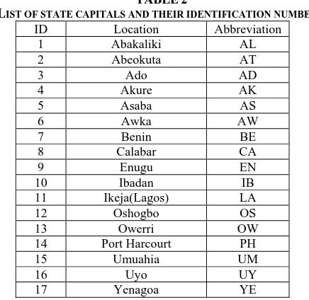
The case study for this work comprises of state capitals in Southern Nigeria, which covers three geopolitical zones in Nigeria. The zones are South, East, and South-West with seventeen state capitals altogether. The list of the state capitals is given in Table 2 with the abbreviation. In the case study, unique identification numbers (ranging from one to seventeen) are used to represent each state capital in alphabetical order as follows: (1, 2, 3, 4, 5, 6, 7, 8, 9, 10, 11, 12, 13, 14, 15, 16, 17), these numbers are arranged in different order randomly to generate several tours. The tours that were generated are then put together and termed the “initial population.”

Table 3 is a chart that shows the distances between the various cities; the first row and column contains the unique identification numbers representing the cities. For instance,”1”represents Abakaliki and “4” represents Akure, as given in Table 2. The number in each cell is the distance between city i and city j. The diagonal cell of the chart is always zero because it contains the distance between a city and itself. Some of the paths in this chart can also be represented as a weighted graph as shown in figure 4.

Figure 2 shows the architecture of the system hybrid genetic algorithm-based model for solving travelling salesperson‟s problem. The architecture shows the different components (functionality) of the system and how they interact. The initial population generated randomly is referred to as the first generation and they are stored in the database for subsequent usage. Evaluation of fitness is performed on the stored generation to obtain good individuals which will be

considered for reproduction. The poor or low rated individuals are removed. Sequential constructive crossover (SCX) is

carried out on the selected individual to produce another generation, which is referred to as the next generation

3.1

Genetic Representation and Coding

The method for representing solutions in genetic algorithm varies from problem to problem but for TSP, solution is typically represented by chromosome of length as the number of nodes in the problem. Each gene of a chromosome takes a label of node such that no node appears twice in the same chromosome. There are mainly two representation methods for representing tour in the TSP which includes adjacency representation and path representation. The authors consider path representation method which simply lists the label of nodes. For example, let “1, 2, 3, 4, 5, 6, 7” be the labels of nodes in a seven node instance, then a tour “1→ 4→ 3→ 5→ 7→ 6→ 2→1” may be represented as (1, 4, 3, 5, 7, 6, 2).

TABLE2

LIST OF STATE CAPITALS AND THEIR IDENTIFICATION NUMBERS.

ID Location Abbreviation

1 Abakaliki AL

2 Abeokuta AT

3 Ado AD

4 Akure AK

5 Asaba AS

6 Awka AW

7 Benin BE

8 Calabar CA

9 Enugu EN

10 Ibadan IB

11 Ikeja(Lagos) LA

12 Oshogbo OS

13 Owerri OW

14 Port Harcourt PH

15 Umuahia UM

16 Uyo UY

[image:4.595.323.541.82.294.2]

17 Yenagoa YE

[image:4.595.314.554.324.509.2]

15

3.2

Objective function and the fitness

function

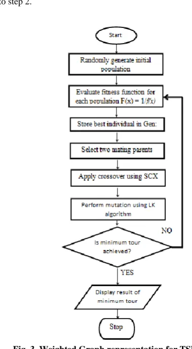
The objective function and the associated constraints are stated in the mathematical formulation of the problem in equation (2), that is, to minimize tour subject to these constraints (3 – 6). One way of defining the fitness function for a minimization problem as stated in [25] is F(x) = 1/f(x), where f(x) is the objective function which calculates the value of tour represented by a chromosome. The hybrid model flowchart description is shown in figure 3 while the weighted graph representation of the travelling salesperson tour is shown in figure 4 respectively.

3.3

Generate Initial Population

The first step in the algorithm is to randomly generate initial population that is possible solutions to the problem, after which the fitness of the individual solution generated is evaluated using the fitness function F(x) = 1/f(x) where f(x) calculates the value of the distance represented by each chromosome. For example, in the case study the f(x) for one of the chromosomes with the following path (1,9,15,16,8,13,6,5,7,4,3,10,11,2,12,14,17) is 2,368Km, hence F(x) = 1/ 2368. Best individuals are then stored as the first generation. The next step is to select two parent chromosomes for mating based on their fitness value.

3.4

Crossover Operation

Crossover operation is applied to the selected chromosomes. The crossover operation used is called Sequential Constructive operator (SCX) as illustrated in [25]. The following steps are;

Algorithm 2:

Step 1: Start from the first node

Step 2: From the first node search both parent chromosomes orderly and pick the node yet to be visited after „node x‟ in each parent. If there is no „node x‟ in any of the parent, search sequentially the nodes that follows and consider the first „legitimate node‟ and go to step3.

Step 3: Suppose the „node a‟ and „node b‟ are found in first and second parents respectively, then for selecting the next node go to step 4.

Step 4: If Cxa<Cxb, then select „node a‟ otherwise, „node b‟ as the next node and add it to partially constructed child (PCC) chromosome. If the child is a complete chromosome, then stop. Otherwise, rename the present node as „node x‟ and go

to step 2.

Sequential Crossover Operation

The SCX is illustrated by selecting a pair of chromosomes from the kilometer chart of the case study given in table 3. Let P1 and P2 be the selected chromosomes with values 6,332Km and 5945Km respectively.

[image:5.595.317.507.79.423.2]

P1: (1, 5, 7, 3, 9, 13, 11, 17, 15, 10, 6, 12, 8, 4, 2, 16, 14) P2: (1, 16, 2, 6, 4, 12, 8, 10, 14, 15, 11, 7, 13, 9, 5, 3, 17)

Table 3

A Kilometer Chart For State Capitals In Southern Nigeria.

1 2 3 4 5 6 7 8 9 10 11 12 13 14 15 16 17 1 0

2 632 0 3 487 271 0 4 482 256 47 0 5 360 416 317 256 0 6 153 486 347 308 52 0 7 316 345 210 171 130 187 0 8 146 733 594 555 299 276 422 0 9 93 560 333 382 127 77 250 263 0 10 650 141 192 178 406 463 309 712 522 0 11 622 86 310 283 430 487 333 736 546 121 0 12 541 194 118 104 358 414 269 663 473 116 233 0 13 183 605 403 364 109 93 231 208 143 561 541 477 0 14 238 589 490 451 205 189 322 216 232 608 588 563 97 0 15 136 568 429 391 135 112 258 165 124 587 567 503 58 115 0 16 195 651 512 473 217 194 340 95 207 670 650 585 127 135 83 0 17 300 534 435 396 241 218 267 309 269 553 533 508 128 116 186 226 0

16

3.5

Mutation

Operation

with

Lin-Kernighan algorithm

In order to vary the solution space, the authors adapt Lin-Kernighan heuristic [37] for the mutation. The final step is to test for minimum tour value. If the minimum tour value is achieved, the result is displayed and the algorithm is terminated else go back to step 2 of Figure 3 and repeat the subsequent steps. The algorithm steps as illustrated in [37] are shown as;

Algorithm 3

ImprovePath(P, depth,R)

Require: The path P = b →. . . →e, recursion depth depth and the set of restricted vertices R.

If depth





then

Find the edge x→y



P, x



b, x



R such that it maximizes the path gain

Gain(P, x →y).

else

Repeat the rest of the procedure for every edge x →y x→y



P, x



b, x



R.

Conduct local search move: P RearrangePath(P, x →y).

If GainIsAcceptable(P, x →y) then

Replace the edge x →y with x →e in P.

T = CloseUp(P).

If w(T ) ≥w(T ) then

Run T ←ImprovePath(P, depth + 1,R



{x}).

If w(T ) < w (T ) then return T

else

Restore the path P.

return T

Note RearrangePath(P, x →y) removes an edge x→y from a path P and adds the edge x →e, where P = b →. . . →x →y →. . . →e. GainIsAcceptable(P, x →y) determines if the gain of breaking a path P at an edge x →y is worth any further effort. CloseUp(P) adds an edge to a path P to produce a feasible tour. ImproveTour (T) is a tour improvement.

4.

IMPLEMENTATION, RESULTS AND

DISCUSSION

4.1

Implementation Results

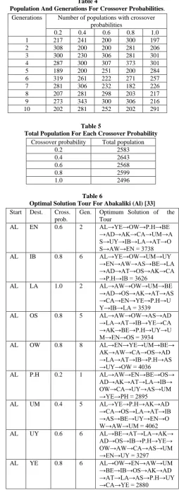
[image:6.595.305.560.82.784.2]

The practical implementation of the hybrid genetic algorithm-based model in solving the travelling salesperson problem, results and comparison with artificial neural network is presented in this section. The algorithm is implemented with Java programming language. The results obtained from the implementation of the algorithm using different crossover probabilities are given in Table 4. The table shows the number of population and generations used for different crossover probabilities while Table 5 contains the summation of the total number of population for each crossover probability used. The population refers to the numbers of individuals that will participate in the crossover operation based on the specified crossover probability in a particular generation. Table 6 shows a sample table for optimum value of tour in a generation with crossover probabilities used from a start location to the destination location. The values in the last column of the table represent the optimal minimum kilometer distance for each tour from Abakaliki (AL). The start and destination locations are abbreviated in two-letters. Figure 5

Table 4

Population And Generations For Crossover Probabilities. Generations Number of populations with crossover

probabilities

0.2 0.4 0.6 0.8 1.0

1 217 241 200 300 197

2 308 200 200 281 206

3 300 230 306 281 301

4 287 300 307 373 301

5 189 200 251 200 284

6 319 261 222 271 257

7 281 306 232 182 226

8 207 281 298 203 217

9 273 343 300 306 216

[image:6.595.52.278.230.446.2]

10 202 281 252 202 291

Table 5

Total Population For Each Crossover Probability

Crossover probability Total population

0.2 2583

0.4 2643

0.6 2568

0.8 2599

1.0 2496

Table 6

Optimal Solution Tour For Abakaliki (Al) [33]

Start Dest. Cross. prob.

Gen. Optimum Solution of the Tour

AL EN 0.6 2 AL→YE→OW→P.H→BE

→AD→AK→CA→UM→A S→UY→IB→LA→AT→O S→AW→EN = 3738

AL IB 0.8 6 AL→YE→OW→UM→UY

→EN→AW→AS→BE→LA →AD→AT→OS→AK→CA →P.H→IB = 3626

AL LA 1.0 2 AL→AW→OW→UM→BE

→AD→OS→AK→AT→AS →CA→EN→YE→P.H→U Y→IB→LA = 3539

AL OS 0.8 5 AL→AW→OW→AS→AD

→LA→AT→IB→YE→CA →AK→BE→P.H→UY→U M→EN→OS = 3934

AL OW 0.8 8 AL→EN→YE→UM→BE→

AK→AW→CA→OS→AD →LA→AT→IB→P.H→AS →UY→OW = 4036

AL P.H 0.2 1 AL→AW→EN→BE→OS→

AD→AK→AT→LA→IB→ OW→CA→UY→AS→UM →YE→PH = 2895

AL UM 0.4 5 AL→YE→P.H→AK→AD

→CA→OS→LA→AT→IB →AS→BE→UY→EN→O W→AW→UM = 4062

AL UY 0.6 6 AL→BE→AT→LA→AK→

AD→OS→IB→P.H→YE→ OW→AW→CA→AS→UM →EN→UY = 3297

AL YE 0.8 6 AL→OW→EN→AW→UM

→BE→IB→OS→AK→AD →AT→LA→AS→P.H→UY →CA→YE = 2880

17 depicts a chart showing a summary of total number of

population used for different crossover probabilities.

4.2

Performance

Evaluation

between

Hybrid GA and Neural Network

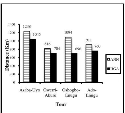
The comparison is done based on two major metrics which are “minimum distance” and “run time”. The distance achieved in a particular tour is obtained by the summation of all the distance values between the cities involved in the tour. Hence, the minimum distance achieved by a particular method is the total distance of a tour with the lowest value. In the comparison, ranges of cities chosen are between 4 and 8 cities because of the computational complexity of ANN. In order to show the efficiency of the HGA an experiment involving a four- city tour and an eight- city tour from the case study is carried out using the ANN and HGA. The result presented in figure 6 shows that HGA is more efficient in terms of minimum distance achieved. The run time (in milliseconds) is the time for a particular method to complete its search. Figure 7 shows the results for the time taken for the both methods to complete their execution. It is could be observed that HGA performs better than ANN.

5.

CONCLUSION

This paper explores the mutation operation process of a genetic algorithm to achieve optimal solutions for the stated Travelling Salesperson Problem. The TSP problem seems to be simple conceptually but may be computationally explosive

to solve. Various approximate techniques had been applied to the TSP. Achieving optimal solution in terms of minimum tour distance and run time had always being motivation for more heuristic approaches.

In this study, Lin-Kernighan algorithm is incorporated into GA to perform the mutation operation. Also, sequential constructive crossover (SCX) method is adopted and used to perform the crossover operation. The HGA model developed is tested with problems from the case study of 17 state capital cities in Southern Nigeria. The HGA model is also compared with ANN model and the result shows that the proposed HGA performed better than ANN in terms of minimum tour distance and run time.

Future scope of research lies in the study of large TSP using other hybrid heuristics. Also optimization of initial population selection and crossover operation processes need to be investigated.

6.

ACKNOWLEDGMENTS

The authors wish to acknowledge the staff and postgraduate students of Computer Science Department, Federal University of Technology Akure, Nigeria for their various support and suggestions during the duration of this research

7.

REFERENCES

[1] Corwin, B. D. and Esogbue, A. O., 1974. Two Machine flow shop scheduling problems with sequence dependent setup times: a dynamic programming approach, J. Naval Research Logistics. Vol. 21, pp. 515-524.

[2] Psaraftis, H. N., 1998. Dynamic vehicle routing problems, In: B. L. Golden, A. A. Assad, (eds.) Vehicle Routing: Methods and Studies, Elsevier, Amsterdam, pp. 223–248.

[3] Li, C. Yang, M. and Kang, L. 2006. A New Approach to Solving Dynamic Traveling Salesperson Problems. In: T.-D. Wang, X. Li, S.-H. Chen, X. Wang, H. Abbass, H. Iba, G. Chen, X. Yao, (eds.) SEAL 2006. LNCS, Springer, Heidelberg, vol. 4247, pp. 236–243.

[image:7.595.320.541.125.315.2]

[4] Guntsch, M. Middendorf, M. and Schmeck, H. 2001. An ant colony optimization approach to dynamic TSP. In: Lee Spector et al., editor, Proceedings of the Genetic and Evolutionary Computation, Conference (GECCO-2001), San Francisco, California, USA, 7-11 July 2001. Morgan Kaufmann, pp. 860–867.

[image:7.595.58.280.300.700.2]

Fig. 5: A graph of total number of population used for different crossover probabilities

Fig. 6: Comparison of minimum distance obtained for four tours using ANN and HGA

1238

816

1094

911 1045

704 696 760

0 200 400 600 800 1000 1200 1400

Asaba-Uyo Owerri-Akure

Oshogbo-Enugu

Ado-Enugu

Distan

ce

(Km)

Tour

ANN

HGA

Fig. 7. Comparison of based on runtime for four tours using ANN and HGA

11 53

111 180

381 580

8 31

84 107

121 125

0 100 200 300 400 500 600 700

3 4 5 6 7 8

Ru

ntime (mil

li

sec

ond

s)

Number of Cities

ANN

[image:7.595.57.278.309.438.2] [image:7.595.61.281.474.673.2]

18 [5] Tabatabaee, H. 2015. Solving the traveling salesperson

problem using genetic algorithms with the new evaluation function, Bulletin of Environment, Pharmacology and Life Sciences, Vol. 4, No. 11, pp. 124-131.

[6] Zukhri, Z. and Paputungan, I. V. 2013. A Hybrid Optimization Algorithm based on Genetic Algorithm and Ant Colony Optimization, International Journal of Artificial Intelligence & Applications (IJAIA), Vol. 4, No. 5, pp. 63 - 75, DOI : 10.5121/ijaia.2013.4505

[7] Jingui, L. Ning, F. Dinghong, S. and Congyan, L. 2007. An Improved Immune-Genetic Algorithm for the TSP In Proc. IEEE Int. Conf. Natural Computation.

[8] Wang, S. and Zhao, A. 2009. An Improved Hybrid Genetic Algorithm for Traveling Salesperson Problem, In IEEE Proc. Int. Conf. Computational Intelligence and Software Engineering.

[9] Rodriguez, M. A. V. Gutierrez-Gil, R. Avila-Roman, J. M. Sanchez-Perez, J. M. and Gomez-Pulido, J. A. 2005. Genetic Algorithms Using Paralelism and FPGAs: The TSP as Case Study, in IEEE Proc. Int. Conf. Parallel Processing Workshops.

[10] Gharehchopogh, F. S. Maleki, I. and Farahmandian, M. 2012. New Approach for Solving Dynamic Travelling Salesman Problem with Hybrid Genetic Algorithms and Ant Colony Optimization, International Journal of Computer Applications, Vol. 53, No. 1, pp. 0975 – 8887. [11] Li-Ying, W. Jie, Z. and Hua, L. 2007. An Improved

Genetic Algorithm for TSP, In IEEE Proc. Int. Conf. Machine Learning and Cybernetics.

[12] Sze, S. N. 2004. Study on Genetic Algorithms and Heuristic Method for Solving Traveling Salesman Problem, M.S. dissertation, Faculty of Science, Universiti Teknologi Malaysia, Johor, Malaysia.

[13] Wang, S. and Zhao, A. 2009. An Improved Hybrid Genetic Algorithm for Traveling Salesperson Problem, In IEEE Proc. Int. Conf. Computational Intelligence and Software Engineering.

[14] Yingzi, W. Yulan, H. and Kanfeng, G. 2007. Parallel Search Strategies for TSP‟s using a Greedy Genetic Algorithm, in IEEE Proc. Int. Conf. Natural Computation.

[15] Zhenchao, W. Haibin, D. and Xiangyin, Z. 2009. An Improved Greedy Genetic Algorithm for Solving TSP, in IEEE Proc. Int. Conf. Natural Computation.

[16] Yan, X. Zhang, C. Luo, W. Li, W. Chen, W. and Liu, H. 2012. Solve Traveling Salesman Problem Using Particle Swarm Optimization Algorithm, IJCSI International Journal of Computer Science Issues, Vol. 9, Issue 6, No. 2, pp. 264-271.

[17] Zhang, C. Sun, J. Wang, Y. and Yang, Q. 2007. An Improved Discrete Particle Swarm Optimization Algorithm for TSP, Proceedings of Web Intelligence/IAT Workshops, pp. 35-38.

[18] Rajasekaran, S. and VijayalakshmiPai, G. A. 2010. Neural Networks, Fuzzy Logic and Genetic algorithms Synthesis and applications, PHI Learning private Limited, New Delhi.

[19] Alireza, A. A. Naserasadi, A. and Zeinab, A. A. 2011. A New Hybrid Algorithm for Traveler Salesman Problem based on Genetic Algorithms and Artificial Neural Networks, International Journal of Computer Applications, Volume 24, No.5, pp. 0975 – 8887. [20] Potvin, J-Y. 1996. Genetic algorithms for the traveling

salesman problem, Annals of Operations Research, Vol. 63, pp. 339-370.

[21] Katayama, K. and Sakamoto, H. 2000. The Efficiency of Hybrid Mutation Genetic Algorithm for the Travelling Salesman Problem, Mathematical and Computer Modeling, Vol. 31, pp. 197-203.

[22] Liu, S. 2014. A Powerful Genetic Algorithm for Traveling Salesman Problem, Proceedings of the course Principles of Artificial Intelligence, Sun Yat-sen University, Guangzhou, China, pp. 1 – 5.

[23] El-Mihoub, T. A. Hopgood, A. A. Nolle, L. and Battersby, A. 2006. Hybrid Genetic Algorithms: A Review, Engineering Letters, 13:2, EL_13_2_11 (Advance online publication).

[24] Donald, D. 2010. Travelling Salesman Problem, Theory and Applications, InTech,Janeza Trdine 9, 51000 Rijeka, Croatia.

[25] Zakir, H. A. 2011. Genetic algorithm for the travelling salesman problem using sequential constructive crossover operator, International Journal of Biometrics and Bioinformatics (IJBB), Vol.3, Issue.6, pp. 96-105. [26] Oluwadare, S. A. 2009. A Scheduling Algorithm for

enhancing operating system support for high-speed multimedia systems, Ph.D. Thesis, Dept. Comp. Sci., Federal University of Technology, Akure, Nigeria.

[27] Raza, Z. and Vidyarthi, D. P. 2009. A computational grid scheduling model to minimize turnaround using modified GA, International Journal of Artificial Intelligence, Vol. 3, No. A9, pp. 86-106.

[28] Johnson, D. S. and McGeoch, L. A. 1995. The Traveling Salesman Problem: A Case Study in Local Optimization, Department of Mathematics and Computer Science, Amherst College, Amherst, MA 01002.

[29] Graupe D. and Gandhi, R. 2001. Traveling Salesman‟s Problem Solution using Hopfield Neural Network, Final year Project Report, ECE 559.

[30] Laarhoven, P. V. and Aarts, E. H. L. 1987. Simulated Annealing: Theory and Applications, KluwerAcademic.

[31] Zhao, F. G. Sun, J. S. Li, S. J. and Liu, M. W. 2009. A Hybrid Genetic Algorithm for the Travelling Salesman Problem with Pickup and Delivery, International Journal of Automation and Computing, Vol. 6, No.1, pp. 97-102, DOI: 10.1007/s11633-009-0097-4.

[32] Tsai, C-W. Tseng, S-P. Chiang, M-C. Yang, C-S. and Hong, T-P. 2014. A High-Performance Genetic Algorithm: Using Traveling Salesman Problem as a Case, Hindawi Publishing Corporation, The Scientific World Journal, Vol. 2014, Article ID 178621, pp. 1-14, http://dx.doi.org/10.1155/2014/178621.

19 [34] El-Mihoub, T. A. Hopgood, A. A. Nolle, L. and

Battersby, A. 2006. Hybrid Genetic Algorithms: A Review, Engineering Letters, 13:2, EL_13_2_11 (Advance online publication)

[35] Helsgaun, K. 1998. An Effective Implementation of Lin- Kernighan Traveling Salesman Heuristic, A Report, Dept. of Comp. Sci., Roskilde Uni., Roskilde, Denmark,http://citeseerx.ist.psu.edu/viewdoc/download? doi=10.1.1.25.4908&rep=rep1&type=pdf.

[36] Saranya, M. and Dhinakaran, S. 2013. Implementation of Traveling Salesman‟s Problem Using Neural Network, International Journal of Computer & Organization Trends, Vol. 3, Issue 4, pp. 161-164, ISSN: 2249-2593. [37] Karapetyan, D. 2010. Design, Evaluation and Analysis of

Combinatorial Optimization Heuristic Algorithms, Ph.D Thesis, Dept. Comp. Sci., Royal Holloway College

University of London.