Portfolio Size in Stochastic Portfolio Networks Using Digital Portfolio Theory

(1)

http://dx.doi.org/10.4236/jmf.2013.32028 Published Online May 2013 (http://www.scirp.org/journal/jmf)

Portfolio Size in Stochastic Portfolio Networks

Using Digital Portfolio Theory

C. Kenneth Jones

Portfolio Selection Systems, Gainesville, USA Email: kenjones@portfolionetworks.com

Received January 25, 2013; revised March 24, 2013; accepted April 19, 2013

Copyright © 2013 C. Kenneth Jones. This is an open access article distributed under the Creative Commons Attribution License, which permits unrestricted use, distribution, and reproduction in any medium, provided the original work is properly cited.

ABSTRACT

The investment portfolio with stochastic returns can be represented as a maximum flow generalized network with stochastic multipliers. Modern portfolio theory (MPT) [1] provides a myopic short horizon solution to this network by adding a parametric variance constraint to the maximize flow objective function. MPT does not allow the number of securities in solution portfolios to be specified. Integer constraints to control portfolio size in MPT results in a nonlinear mixed integer problem and is not practical for large universes. Digital portfolio theory (DPT) [2] finds a non-myopic long-term solution to the nonparametric variance constrained portfolio network. This paper discusses the long horizon nature of DPT and adds zero-one (0-1) variables to control portfolio size. We find optimal size constrained allocations from a universe of US sector indexes. The feasible size of optimal portfolios depends on risk. Large optimal portfolios are infeasible for low risk investors. High risk investors can increase portfolio size and diversification with little effect on return.

Keywords: Finance; Portfolio Optimization; Portfolio Networks; Asset Allocation; Investment Diversification; Digital Signal Processing; Mixed Integer Programming

1. Introduction

The need for a practical long-term portfolio management decision model is increasing. In addition, the need for more diversification than is recommended by portfolio optimization models has become apparent. Considerable research focuses on short-term conditional volatility models, or suggests using a string of short-term volatility models in multiple periods. Digital portfolio theory (DPT) [2] is a long-term portfolio selection model since it includes non-overlapping mean-reversion variances for different horizons. DPT is a normative model for portfolio optimization that includes the importance of holding period and horizon risk in single period solutions. This paper extends the research of Jones by clarifying the horizon structure of DPT and examines portfolio size constraints to control diversification.

Solutions to the maximum flow, risk constrained portfolio network have focused on using Modern portfolio theory (MPT) [1] to construct mean-variance efficient portfolios. The nonlinear MPT model provides a solution to the generalized portfolio network by adding a parametric quadratic variance side-constraint to the maximize

flow objective function. In practice, MPT solutions are myopic, ill-conditioned, unstable, and are sometimes inappropriate and not intuitive. MPT solutions do not per- mit the user to specify the number of securities in solution portfolios. Adding integer constraints to quadratic MPT is NP-hard with computational effort that grows exponentially with universe size. Conventional portfolio optimization models do not have the capability to apply integer constraints. This is primarily because portfolio theory models are risk constrained optimization models and therefore nonlinear. Controlling portfolio size is not practical since solutions are NP-hard.

(2)

rizon mean-reversions contribute to single period risk. DPT finds single period mean-variance solutions to the long horizon problem. DPT only considers long horizon variance, volatility is not included. DPT represents return stochastic processes as digital signals and the power spectral density (PSD) describes the risk characteristics of the multipliers in the portfolio network. Solutions are more appropriate because they control exposure to long and short horizon variances of calendar and non-calendar length expected returns. The independent control of horizon based variances allow investors to find portfolios that satisfy long and short horizon risk requirements based on their holding periods. For a given holding period investors will have hedging demand for shorter horizon risk and speculative demand for longer horizon risk. Because DPT offers a time dimension to risk assessment, the holding period of the investor plays a significant role in the optimal decision. As holding periods shorten and as markets change, optimal portfolios must be rebalanced to adjust horizon risk levels, to satisfy hedging and speculative demands for mean-reversion risk.

Recent research suggests that the relatively small portfolios found using MPT, or DPT should be larger do the higher volatility in the markets today. In the 1970s 20 randomly selected stocks could eliminate unsystematic risk while in the 1990s it required 50 stocks to eliminated unsystematic risk. An investor’s subjective estimate of the number of securities that should be held in a portfolio may differ markedly from the number recommended by an optimization model. Small portfolios may be subject to individual idiosyncratic (active) risk while very large portfolios may approach an indexing strategy with high passive risk. The larger the portfolio, the larger the bro- kerage fees required to keep it rebalanced. The holding period risk tolerance will have a bearing on the number of assets to be held by a particular investor. Active portfolio managers may prefer concentrated portfolios with fewer securities to capitalize on forecasts. Alternatively passive investors may have longer holding periods, trade less frequently, and prefer larger portfolio sizes.

This paper presents a mean-variance-autocovariance portfolio selection decision support application that allows the number of securities in the optimal portfolio to be pre-specified by the investor. Zero-one variables are used to control portfolio size in the stochastic portfolio network. Size constrained optimal portfolios can be used to meet investors’ diversification objectives. Portfolio managers may have strong convictions regarding the size of their portfolios. Integer constraints can be used to find larger optimal portfolio solutions resulting in more diversification. Alternatively smaller portfolios can be found to benefit from special situations and still achieve optimal diversification. Zero-one integer side-constraints and DPT allow control of optimal portfolio size, turnover,

and diversification. Integer constraints can also be used to include fixed trading costs in optimal portfolio solutions [3].

The paper defines and tests portfolio optimization solutions assuming the stochastic portfolio network model is the appropriate representation of the problem and DPT gives the best solution when expected returns are time- varying. In the DPT problem non-integer variables are used to solve for maximum portfolio return while constraining calendar and non-calendar length mean-reversion risk. Integer variables are used to control portfolio size. The optimal solution will depend on risk profile and portfolio size preference. The risk profile will depend on the investors holding period and hedging and speculative demands for mean-reversion risk. The mixed integer DPT solution finds optimal portfolios based on the investors preferences with respect to portfolio size, horizon risk, systematic risk, and unsystematic risk. We test the DPT model with zero-one constraints and find it effec- tive in identifying size constrained optimal asset allocations. Low risk investors are constrained to small portfolios while high risk investors can hold large portfolios with small reduction in return.

2. Stochastic Generalized Portfolio Networks

Figure 1 shows the one-period generalized portfolio network [4,5]. The multipliers represent return and are uncertain or stochastic. When the input to the portfolio at node 0 is constrained to be one the output of the portfolio network from node 1 is the stochastic portfolio return. In this portfolio network we are assuming no negative flows (short sales) and no arcs from right to left representing borrowing or leverage. Jones [6] has examined these cases in the stochastic portfolio network framework. The maximum flow network is the natural structure for the return maximization portfolio selection problem. The arc flows, wj, are constrained to represent percentages of the initial investment.

3. Modern Portfolio Theory

(3)

[image:3.595.59.287.81.198.2]

 1,1 0 1 1 w 2 w 3 w N w 1 r 2 r 3 r N r p r

Figure 1. The single period stochastic generalized portfolio network.

mean flow. The MPT maximum flow problem is,

 







 



1 1

max

N N

p j j j j

j j

E r t w E r t w

 









  (1)

In order to control portfolio risk MPT adds a quadratic parametric portfolio variance side-constraint to the maximum flow portfolio network in Figure 1, subject to

 







   



1 1

var _p N N _i _jcov _i , _j

i j

r t w w r t r t B

 





    , (2)

1 1 N j j w  



, (3)

0 1, 2,3, j

w  j N. (4) where wj is the fraction invested in security j, r t_p

 

is the stochastic return on the portfolio in period t, N is the number of securities in the potential universe, and B is a right-hand side (RHS) constant. The quadratic constraint (2) controls the portfolio risk or variance of expected returns at node 1. As the value of B, the right-hand-side, is changed the optimal solution to the nonlinear-programming problem will trace out the mean-variance efficient set. The problem is convex and the solution consid-ers all portfolio combinations until a global mean-variance efficient portfolio is found. This is defined as the portfolio of securities with the highest level of expected return at a specified portfolio variance level. The optimal portfolio for a particular investor depends on the investor’s desired exposure to portfolio variance. Constraint (3) is the flow conservation equation at node 0 called the budget constraint. The last constraint (4) restricts short selling, or negative arc flows in the portfolio network.

Adding multiple zero-one variables to the MPT model to control optimal portfolio size results in a mixed integer quadratic programming problem and therefore is rarely implemented. The use of zero-one variables considerably increase the time required to find the optimal solution. When zero-one variable constraints are added to MPT it is difficult to reach a solution in a reasonable amount of time unless the universe size is small. In addition, MPT

finds inappropriate solutions or “unnatural portfolios” primarily because stock prices do not follow a random walk. Expected returns have been found to be mean-re-verting, not normally distributed, and subject to high estimation error. The covariance matrix is unstable in time and the assumptions of constant expected return and zero autocorrelation are not realistic. Fortunately DPT is a more robust model that is not only linear but allows control over the long-term variance of the stochastic portfolio return process.

4. Digital Signal Processing

Digital portfolio theory (DPT) uses the mean-variance framework to find risk constrained optimal portfolios in the portfolio network. DPT uses low frequency digital signal processing (DSP) to describe the stochastic return processes of the portfolio network multipliers in Figure 1. It does not require returns to be iid but instead it assumes that stock return processes are stationary. To apply DSP, finite sequences of returns or signals describe return processes rather than single period returns. The digital return signal, r n

 

consists of a sequence of returns of length T,

 

1, 2,3, .

i

r n n T (5)

The square brackets indicate a digital process. The integer n indicating the place in the sequence and r nj

 

is

the stochastic return at time nδt for asset j. The equal time interval between returns is δt. T gives the finite signal length of the return signal. Digital return signals are constructed from discontinuous prices and dividends. Every vector of returns of length T is assumed to be a realization of a stationary random process,

 



i



E r n i (6) The DSP model utilizes the finite Fourier series to describe the second moments, or variance of the random signals. The Fourier Theorem states that the variance of any finite discrete wide sense stationary (WSS) stochastic process can be described non-parametrically by a finite sum [7]. All return signals have the following characteristics,

 



 



1

exp i 1,2, ,

T

j j

n

R k r n k n k K





    , (7)

 





2



1 1 var 2 K j k

r n R k_j 







 . (8)

In the discrete Fourier transform (7), R kj

 

 , or Rkj is

(4)

interval. Each signal has K mean-reversion variance components that are uncorrelated and form a complete orthogonal set. The total single period variance of a return signal in Equation (8) is the sum of K longer-term variance components, . The K mean-reversion variance components, , describe the power spectral density of the finite return signal’s process. The kth component gives the variance of short or long horizon expected returns and describes the presence of autocorrelation in the return process. Note that the K variance components in Equation (8) are time-invariant. The phase information or timing characteristics are not contained in the variance. The expression for the variance (8) is nonparametric. There is no assumption about the distribution of returns they may be skewed, fat tailed, etc.

2 ki

R

2 ki

R

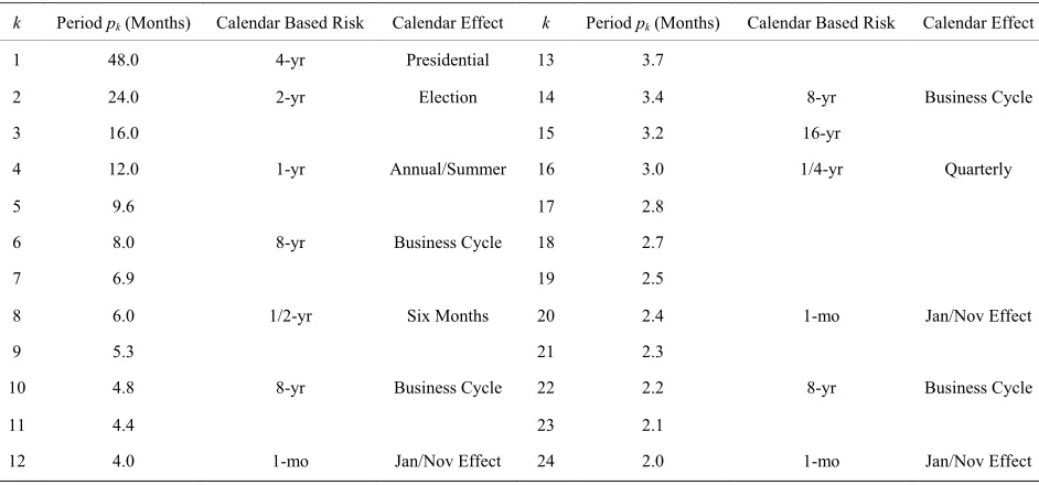
sion lengths cannot be measured directly with monthly data using DSP, monthly mean-reversion risk is reflected in periods related to; 2-month, 2.4-month and 4-month periods. The variance of longer horizon returns such as 8-year and 16-year risk is reflected in shorter harmonics. Using monthly sampling shorter horizon length volatil- ities such as weekly, daily, second, microsecond, or con- tinuous are not measured.

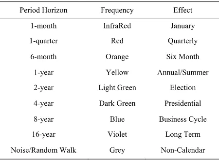
Table 2 shows how calendar length mean-reversions can be related to the colors of visual light. Signal processing refers to a stochastic process that is not white noise as colored noise. Samuelson [8] suggested the pos- sibility of red versus blue noise. Stock price changes may have short-term mean-reversion (red noise) or much longer-term mean-reversion (blue noise). Table 2 gives a color-coding for mean-reversion risk corresponding to the visual light spectrum.

The horizon length of the kth mean-reversion variance component, pkis a function of the signal length and the

index k, Each mean-reversion variance component, in (8)

relates to the risk of all returns computed over the corresponding period length. Using DSP the fundamental period, or signal length must be chosen to match the un- derlying process generation. For this reason signal lengths must be one year, two years, four years, or eight years using monthly returns. For a 48-month signal the variance component for k = 4, with period p4 = 12-

months, will be larger when returns measured over one- year holding periods have a larger variance. The 12- month variance measures the variance contributed by one year mean-reversions contained in the signal. The 48- month variance is the risk in the process contributed by four-year holding period returns. The three-month variance is the risk related to three month mean-reverting

2 ki

R

1, 2, , 2

k

[image:4.595.63.534.497.717.2]

p T t k k   K T t. (9) The period lengths decrease harmonically. Calendar based mean-reversion risk can be defined as the variance of expected returns having a period with length related to a calendar time interval. We use a sampling interval of one month because it is generally the shortest company reporting interval. Using monthly returns with a T = 48 month (four-year) signal length, Table 1 shows 24 independent calendar and non-calendar mean-reversion risk periods and their economic effect. Calendar mean-reversion risks have lengths of monthly, quarterly, 6-month, annual, 2-year and 4-year return horizons. Because the contribution to one month risk of monthly mean-rever-

Table 1. Calendar and non-calendar holding period return horizons.

k Period pk(Months) Calendar Based Risk Calendar Effect k Period pk (Months) Calendar Based Risk Calendar Effect

1 48.0 4-yr Presidential 13 3.7

2 24.0 2-yr Election 14 3.4 8-yr Business Cycle

3 16.0 15 3.2 16-yr

4 12.0 1-yr Annual/Summer 16 3.0 1/4-yr Quarterly

5 9.6 17 2.8

6 8.0 8-yr Business Cycle 18 2.7

7 6.9 19 2.5

8 6.0 1/2-yr Six Months 20 2.4 1-mo Jan/Nov Effect

9 5.3 21 2.3

10 4.8 8-yr Business Cycle 22 2.2 8-yr Business Cycle

11 4.4 23 2.1

12 4.0 1-mo Jan/Nov Effect 24 2.0 1-mo Jan/Nov Effect

(5)

[image:5.595.60.285.101.266.2]

Table 2. Risk based on mean-reversion horizon. Period Horizon Frequency Effect

1-month InfraRed January

1-quarter Red Quarterly

6-month Orange Six Month

1-year Yellow Annual/Summer

2-year Light Green Election

4-year Dark Green Presidential

8-year Blue Business Cycle

16-year Violet Long Term

Noise/Random Walk Grey Non-Calendar

a_{Short, intermediate, and long-term mean-reversion calendar lengths can be} described by a 4-year signal with a monthly observation horizon. The visual color spectrum can be used to represent economically meaningful mean- reversion horizon lengths. Multiple seasonal and cyclical effects as well as non-calendar effects such as white noise generate one-month variance.

returns. If the stock price process is a random walk the returns will be white noise, all variance components will be equal or insignificantly different, the process will have no mean-reversion, and is memoryless. The calendar components of risk have been found to be statistically significant for individual stock return total variance and idiosyncratic variance [9]. These longer periodic risk components in Table 1 do not describe volatility. Vola- tility is a small component of total risk. It is relevant to the high frequency trader with a short holding period.

Unlike MPT or intertemporal portfolio theory, DPTis not a volatility model useful for the short-term trader. By measuring the variance of long and short horizon returns in Equation (8) and Table 1, DPT allows the portfolio risk characteristics to be adjusted to suit the long-term investor’s holding period and time dependent expecta- tions.

5. Digital Portfolio Theory

Digital portfolio theory (DPT) uses a relaxation of the portfolio variance constraint represented in the frequency domain to find efficient portfolios with an LP solution. The derivation of DPT can be found in [2,6], and [4]. The objective of DPT is to maximize the expected portfolio return flow from node 1 in Figure 1 for the one period portfolio network subject to constraints on various mean-reversion variance contributions to the portfolio. The inclusion of mean-reversion risks means that the optimal single period portfolio for a particular investor will depend on holding period. The DPT formulation is:

 





1

max

,

N

p j j

j

E r t w









, (15)

0 1, 2,3, ,

j

w  j  N . (16)

where

µj = expected return for security j, wj = solution weight of security j,

N = number of securities in the asset universe,

Rkj = standard deviation (amplitude) of the kth periodic returns in return signal j,

θkmj = kth phase-shift (correlation) between index m and security j’s return signals,

K = 1/2 the signal length T (K = 24, T = 48 months), cβk = constant that limits the systematic risk of period k portfolio returns,

cαk = constant that limits unsystematic risk of period k portfolio returns.

Equations (10) to (16) describe the DPT model formulation. It is a completely linear model and allows much greater control over the components of portfolio variance. In the case of a 48-month signal length, there are 24 mean-reversion risk components as shown in Table 1 resulting in 96 constraints. These risk constraints do not change with time because all return processes are as-sumed to have stationary second moments. Portfolio risk is time invariant while returns and risk premiums are time-varying. The constraints do not depend on the dis-tribution of returns since return signals are described non-parametrically. This description of portfolio variance includes information about multiple mean-reversions or autocorrelations of all securities in the universe.

[image:5.595.318.540.102.320.2]

(6)

recent years the markets have demonstrated that a mean- reversion risk hypothesis is more appropriate than the random walk hypothesis.

DPT uses four constraints for each holding period risk component. The first two constraints (11) and (12) control the upper and lower bounds on systematic risk (cosine terms), and the second two risk constraints (13) and (14) control upper and lower bounds on unsystematic risk (sine terms). Constraint (15) is the flow conservation condition at node 0 in Figure 1. Constraint (16) prohibits negative arc flows. The DPT model incorporates the correlation structure in K = 24 calendar and non-calendar independent dimensions rather than in one dimension. The covariance structure is measured relative to an index process and is therefore more stable and significant than the MPT covariance matrix. By choosing appropriate values of the right-hand-side (RHS) constants cβk and cαk, DPT allows diversification to be applied independently to the different mean-reverting, systematic and unsystematic risk factors that make up the optimal portfolio variance.

DPT incorporates the risk that long-term mean-reversion contributes to single period risk. DPT gives a horizon based non-myopic solution. For a multiperiod investor the optimal risk return trade off depends on holding period when returns are mean-reverting. To reduce the variance of terminal wealth and to hedge against the pos- sibility that unexpected patterns will benefit returns, investor will have hedging demands for mean-reversion variances with periods shorter than, or equal to their holding period. In addition, investors may have speculative demand for mean-reversion variances longer than their holding period. There are separate risk return utility functions for each mean-reversion risk component. The concept of time diversification suggests that we should hold higher risk portfolios the longer the holding period. Investors will have intertemporal hedging demand for risk when their holding period is greater than or equal to the mean-reversion length. We can hedge against being caught holding cash in unexpected market movements by increasing mean-reversion risk for periods shorter or equal to our holding period. An asset with mean-reversion length less than, or equal to the holding period will reduce the variance of terminal wealth.

If the mean-reversion length is greater than the holding period we may have intertemporal speculative demand for this long horizon risk. With no short selling we can speculate by increasing long-term mean-reversion risk in a rising market (momentum strategy) or we can speculate by deceasing long-term mean-reversion risk in falling market (hold cash and try to buy at a lower price). Indi- vidual utility functions for hedging risks will not neces- sarily be the same as utility functions for speculative risks. DPT is a non-myopic strategic asset allocation

model because it takes into account information beyond the current period. It assumes that mean-reversion risks can be forecast.

Optimal risk depends on holding period. For example, suppose we have a one-year holding period. Our risk return utility function for 3-month risk will be influenced by hedging demand while our risk return utility function for 16-year risk will depend on speculative demand. In- vestors’ utility functions for horizon dependent risk components will depend on holding period. Hedging demands will apply to more mean-reversion components the longer the holding period (time diversification). As time passes our holding period will become shorter and our hedging demand will be for shorter and shorter mean-reversion lengths. In the last period the hedging demand will be small while speculative demand for longer mean-reversion risks will dominate our decision. Non-calendar length risks, since they are not signifi- cantly different from those generated by a random walk [9], will not be subject to hedging demands and therefore a myopic low risk strategy can be applied to these risk components.

The digital formulation uses 96 constraints to control the 24 independent periodic components of risk. The phase-shift, θkmj is estimated using the cross spectral density between the security’s return signal and the index return signal. The cosine and sine terms in Equations (11) to (14) are related to the time domain. The cosine of the phase shift, θkmj is equal to the correlation between the kth independent mean-reverting return components of both processes,

1 kmj coskmj 1

    , (17)

ρkmj = correlation of security j with the index portfolio m’s k-period returns.

In the MPT paradigm, stock price processes follow a random walk; in the DPT paradigm [2] stock return processes may be mean-reverting. The sum of multiple stationary waves of risk produces changing returns in calendar or non-calendar patterns. DPT only quantifies the risk that patterns occur but makes no attempt to de- termine what patterns other than their mean-reversion length. The inclusion of mean-reversion lengths and their risk make DPT a truly long-term portfolio selection model. The risk in the current period is a result of multiple length mean-reversions.

(7)

correlations. In addition, the total number of terms used in DPT grows linearly with universe size while it grows exponentially for MPT. Because the DPT objective function is not quadratic it can be modified or weighted to adjust for compounding, or to allow geometric mean, growth optimal, or momentum objective functions.

Portfolio size constraints can be combined with other portfolio constraints. Additional upper and lower bounds on individual securities or asset classes can be included. Integer constraints can explicitly limit turnover and re- balancing. The DPT formulation is used to derive posi- tive long-term equilibrium theories, or horizon based asset pricing models (see [6,10]). A DPT software program was published by Jones [11]. This paper adds integer constraints to control portfolio size and diversification.

6. Specifying Portfolio Size

This section derives the portfolio selection decision that allows the number of securities in the optimal portfolio to be specified by the investor. This allows control of the size, turnover, and diversification of the optimal portfolio. Zero-one variables are practical in the portfolio network model using DPT since it is linear and allows large universe optimally diversified solutions. In order to apply a zero-one constraint we first define zero-one variables for each security in the security universe,

1, , , ,2 3 N where j 0 or 1.

z z z  z z  (18) These zero-one variables are linked to the percent weights flowing on the investment arcs in the portfolio network in Figure 1. When a weight is zero the corresponding zero-one variable is zero, when a weight is greater than zero the zero-one variable will be one (assuming no short selling). In order to ensure that these conditions are met, the following side-constraints must be added to the portfolio network and the DPT model in Equations (10) to (16):

1 1

2 2

0 0

0

N N

w z

 

 (19)

The constraints in (19) insure that when security j is included in the portfolio and the percent flow on the investment arc wj is greater than zero, the zero-one variable zj will be 1. Since 0 ≤wj≤ 1 from constraints Equations (15) and (16) the above constraints ensure that wj > 0 only if zj = 1. If zj = 0, then wj must equal zero since wj ≥

0.

The following additional constraints must be added to insure that when security j is not included in the portfolio and percent flow wj is zero on investment arc j, the cor-

responding zero-one variable, zj will be zero:

1 1

2 2

0 0

0

N N

w Lz w Lz

w Lz

   

 

 (20)

In addition to forcing zj to be zero when wj is zero, these constraints allow a minimum investment condition or percentage, L to be imposed on the solutions weights. One problem with both DPT and MPT is that optimal solution weights often include very small allocations to some security or securities. It may not be practical to hold less than one half percent in any particular security in order to justify monitoring costs, etc. The constraints in (20) allow the user to set a minimum investment or lower bound, L on the solution weights. For example, in a one million dollar portfolio one might not want to hold a position smaller than five thousand dollars. To ensure this is true L can be set by the user to 0.005 in constraints (20).

In conjunction with constraints (19) and (20) the zero- one variables can be used in a zero-one constraint to control portfolio size. The following constraint can be added to DPT to adjust the number of securities (S) the user wants in the portfolio,

1

N j j

z S





. (21)

The investor may wish to retain some of their holdings and would like to find the optimal way of creating diversification and maximize expected return. In order to reduce the number of new securities added to a portfolio a turnover constraint in conjunction with lower and upper bound constraints can be added. To retain existing holdings zero-one variables corresponding to these investments can be excluded. Lower and upper bounds on the non-integer variable weights can be preset at the desired allocations. For example, suppose we would like to retain five investments that we currently own. The following constraint can be used, where O is the maximum number of new securities or asset classes to be bought to rebal- ance the portfolio,

6

N j j

z O







. (22)

In some cases the portfolio manager will want to force a minimum number of securities into the portfolio in order to achieve diversification in today’s volatile markets. A diversification constraint can be used to force the minimum number of securities to be greater than or equal to a user specified constant, D,

1

N j j

z





(8)

The diversification constraint in conjunction with lower and upper bounds on non-integer variables (wj) can be used to satisfy policy or regulatory restrictions placed on the portfolio manager to avoid excessive exposure to idiosyncratic risk.

7. Testing DPT with Portfolio Size

Constraints

The returns from 73 indexes and the S&P 500 index compiled by Standard and Poor’s and available in the Compustat database were used for the test universe (see the Table 3). These index portfolios represent the stock returns of all large and medium sized US firms associ- ated by industry sector. This test universe consisted of 65 industry indexes and 8 broader indexes including; the S&P and DJ Industrial indexes, the S&P and DJ Utilities indexes, S&P and DJ Transportation indexes, the S&P Midcap index, and the S&P Financial index. Four Indus- try indexes had missing returns and are excluded; Capital Goods 500, Office Equipment&Supplies 500, Commer- cial and Consumer Service 500, and Food& Health Dis- tributors 500. Portfolio optimization research rarely re- ports actual portfolios, frequently because MPT solutions are difficult to reproduce. In order to make our result comparable we report efficient portfolio for a small number of cases. The DPT parameters were estimated using 16 years of monthly returns for each index from July 1982 to June 1998. Four-year signal lengths and the Welch method were used with a temporal rectangular window to find power spectral density and cross spectral density estimates. The minimum investment, L was constrained in all cases to be a two percent of the initial investment. For these tests all right-hand-side constants, cβk and cαk were set equal for all k in constraints (11) to (14).

[image:8.595.311.536.101.682.2]

Table 4 gives the optimal portfolios for low, medium, and high risk levels before portfolio size constraints are applied. Note that these are horizon neutral, active portfolios since horizon, passive and active risks are constrained equally. They are horizon neutral (not short-term, or long-term) since no holding period is specified. Hedging risks and speculative risks are treated the same. For a given holding period the kth RHSs in DPT will in general be larger for shorter mean-reversion lengths. In- vestors will normally have more demand for hedging risk than for speculative risk. Much of the time, hedging demand for risk will be larger than speculative demand for risk. For most securities systematic risk is much larger than unsystematic risk so equally constraining active and passive risks results in small active portfolios. When active risk is more tightly constrained larger passive portfolios will result with larger allocations to broad market indexes. The optimal minimum-variance portfolio (col-

Table 3. Compustat index database with no missing returns.

Index Index

S&P 500 Comp-LTD Footwear-500

S&P Industrials-LTD Beverages (Alcoholic)-500

Dow Jones Industrials-30 Beverages (Non-Alcohlc)-500

Dow Jones Transportation-20 Brdcast (TV, Radio, Cable)-500

Dow Jones Utilities-15 Entertainment-500

S&P Midcap 400 Index Foods-500

S&P Financial Index Househould Pds(Non-Dura)-500

S&P Transportation Personal Care-500

S&P Utilities Restaurants-500

Aluminum-500 Retail (Drug Stores)-500

Chemicals-500 Retail (Food Chains)-500

Chemicals (Diversified)-500 Tobacco-500

Containers&Package (PPR)-500 Oil&Gas (Drilling&Equip)-500

Gold&Prec Metal Mining-500 Oil (Domestic Integrtd)-500

Iron&Steel-500 Oil (Intl Integrated)-500

Metals Mining-500 Banks (Major Regional)-500

Paper&Forest Products-500 Banks (Money Center)-500

Aerospace/Defense-500 Consumer Finance-500

Containers(Metal&Glass)-500 Insurance (Life/Health)-500

Electrical Equipment-500 Insurance (Multi-Line)-500

Machinery (Diversified)-500 Insurance (Ppty-Cas)-500

Trucks&Parts-500 Savings&Loan Companies-500

Waste Management-500 Hlth Care (Drugs-Mjr Ph)-500

Auto Parts&Equipment-500 Health Care(Hsptl Mgmt)-500

Automobiles-500 Hlth Care (Med Pds&Supp)-500

Building Materials-500 Communication Equipment-500

Hardware&Tools-500 Computers (Hardware)-500

Homebuilding-500 Computer (Software&Svc)-500

Household Furn&Applnce-500 Electronics (Instrumntn)-500

Leisure Time (Products)-500 Electronics (Semicndctr)-500

Lodging-Hotels-500 Airlines-500

Publishing-500 Railroads-500

Publishing (Newspaper)-500 Truckers-500

Rtl (Building Supplies)-500 Electric Companies-500

Retail (Dept Stores)-500 Natural Gas-500

Retail (General Mdse)-500 Oil Composite

Textiles (Apparel)-500 Retail Composite

a_{A universe of 73 indexes and the S&P-500 market index was used with} statistics estimated over the 16-year period 1982 to 1998. The test universe consisted of 65 industry indexes and 8 broad indexes including; the S&P and DJ Industrial indexes, the S&P and DJ Utilities indexes, S&P and DJ Transportation indexes, the S&P Midcap index, and the S&P Financial

(9)

Table 4. Horizon neutral active optimal portfolios.

Optional Solutions

(1) (2) (3) (4) (5) (6) (7) (8) (9) (10) (11)

Risk level Low Low Low Low Med Med Med High High High High

Max E(rp) (% per month) µp 1.43 1.57 1.65 1.88 1.93 2.12 2.21 2.28 2.32 2.33

Portfolio standard deviation σp 3.26 3.41 3.56 4.08 4.26 4.39 4.67 4.95 5.98 7.19

Portfolio Beta βp 0.64 0.69 0.71 0.80 0.76 0.81 0.87 0.85 0.82 0.81

Portfolio size 7 9 9 8 10 9 6 3 2 1

Solution tries NF*_{265 271 253 287 319 295 298 227 168 104}

Sector wj Weight

Dow Jones Utilities-15 Stk 36.3%

Gold&Prec Metal Mining-500 4.9% 2.2%

Containers (Metal&Glass)-500 7.4% 2.6% 5.4%

Automobiles-500 6.6%

Rtl (Building Supplies)-500 12.3% 14.8% 11.1%

Textiles (Apparel)-500 9.6% 15.5% 11.1%

Footwear-500 5.5% 8.0% 2.0%

Beverages (Non-Alcohlc)-500 3.4% 51.5% 65.4% 75.9% 26.2%

Brdcast (TV, Radio, Cable)-500 4.0% 2.2% 16.0% 12.3%

Hourshold Pds (Non-Dura)-500 2.0%

Retail (Food Chains)-500 15.8% 17.6% 19.1% 10.0% 3.5%

Tobacco-500 7.0% 9.3% 8.4% 5.6% 3.8% 5.2%

Oil (Intl Integrated)-500 16.5% 16.5% 19.0%

Insurance (Ppty-Cas)-500 3.3% 6.0% 2.2%

Hlth Care (Drugs-Mjr Ph)-500 43.6% 46.6% 2.0%

Computers (Hardware)-500 11.3% 10.6% 9.3% 8.7% 5.9%

Computer (Software&Svc)-500 2.3% 5.8% 12.9% 73.8% 100%

Electric Companies-500 5.8% 21.4% 13.0%

Natural Gas-500 7.1% 9.7% 11.8% 11.1% 4.5%

Total portfolio weight 0% 100% 100% 100% 100% 100% 100% 100% 100% 100% 100%

Risk constraint settings

Systematic risk RHS (Cβk) 1.25 1.26 1.27 1.30 1.42 1.45 1.60 1.70 1.90 2.50 3.00

Unsystematic risk RHS (Cαk) 1.25 1.26 1.27 1.30 1.42 1.45 1.60 1.70 1.90 2.50 3.00

*_{NF-No feasible solution.}a_{The table shows DPT solution portfolios at 10 risk levels. The first column gives the constraint level at which the solution becomes} infeasible. Column 2 gives the minimum variance portfolio. Rows 2, 3, 4, and 5 give the maximum return objective function value, portfolio total risk, beta and size. Row 6 gives the number of tries to reach the solution using a MIP solver with 2% minimum investment constraint. The bottom 2 rows give the user de-fined constraint RHS constants (cβk = cαk). Since all RHSs are equal there is no distinction between horizon, active, or passive risk. DPT parameters are

esti-ated using a universe of 73 indexes plus the benchmark S&P 500 index with monthly returns from 1982 to 1998. m

(10)

[image:10.595.125.472.471.684.2]

umn 2, σp = 3.26) contained utilities, gold, apparel, food chains, oil, computer hardware, and electric companies. The DJ Utilities, the lowest risk index (σj = 3.77), makes up 36.3% of the optimal minimum-variance portfolio. Gold which has the highest individual risk (σj = 10.56) and the lowest market correlation (ρmj = 0.25) is included only in the lowest risk portfolios. This minimum variance portfolio is a low risk portfolio not a short horizon portfolio. Utilities, for example, have more long-term mean- reversion risk than short-term mean-reversion risk.

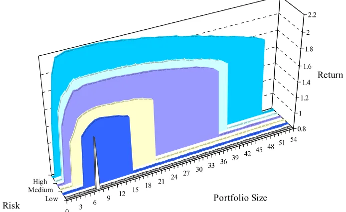
Figure 2 shows feasible portfolio size regions and optimal returns at six risk levels. As portfolio size is changed the optimal portfolio’s expected return falls below the unconstrained optimum holding risk constant. Decreasing portfolio size below optimal reduces return faster than increasing portfolio size. In this US equity sector universe, low total risk optimal allocations are smaller with fewer feasible size possibilities. The lower the risk the fewer portfolio size possibilities were feasible. The minimum-variance optimal portfolio has only one feasible size with seven sector indexes. Feasible solutions at a low risk levels; σp = 3.41 have between 5 and 15 assets. While we might assume that increasing diversification by increasing portfolio size would reduce risk instead we find that large low risk optimal portfolios are not feasible. At lower risk levels increasing diversification by increasing portfolio size is not feasible. In a US sector universe the low risk optimizing investor must hold a small portfolio. An asset allocation with a large number of sectors cannot be an optimal low risk portfolio.

The higher the risk the more portfolio size possibilities are feasible. At medium risks; σp = 4.08 portfolio sizes are feasible for between 2 and 37 indexes. For the high-risk portfolios, σp = 4.67 the upper bound on feasible portfolio size (50) is a function of the minimum investment restriction, L.

8. Conclusions

Virtually every quantitative portfolio manager uses, or is aware of some type of optimization program to provide portfolio recommendations. The majority of these pro- grams cannot find optimal portfolios with portfolio size specified in advance, nor do they incorporate mean-reversion risks and holding period. The majority of indi- viduals and institutions are long-term investors and DPT provides a long-term portfolio optimization framework. Long horizon DPT gives the long-term investor the ability to quantify and control mean-reversion risk levels to satisfy hedging and speculative demands. DPT gives a better understanding of long-term portfolio optimization when returns are mean-reverting. Its application may reduce the focus on short-term volatility. DPT adds a time dimension to portfolio theory and differentiates hedging and speculative risks based on holding period. We examine DPT solutions to the stochastic portfolio network with zero-one constraints to control portfolio size. At a given risk level changing portfolio size from the unconstrained solution size is accomplished at the expense of the portfolio expected return. The ability to find optimal size constrained portfolios depends on the

0 3

6 9

12 15 18 21

24 27 30 33

36 39 42 45

48 51 54

Low MediumHigh

0.8 1

1.2 1.4 1.6 1.8

2 2.2

Return

Portfolio Size Risk

Figure 2. Feasible portfolio size regions, total risk, and optimal return. aThis figure shows the minimum-variance portfolio (front) and 5 increasing risk level optimal portfolio feasible regions. The portfolio size constraint is changed to find the feasi-ble regions at each risk level. The minimum-variance portfolio has only one feasifeasi-ble size (7 securities). The low risk portfolio

s feasible for between 5 and 15 assets with a larger range of feasible portfolio sizes at higher risk levels. i

(11)

level of risk exposure required by the investor. In a universe of US sector and broad market equity indexes, portfolio optimization is more important for the low risk investor than the high risk investor. Low risk optimal asset allocations cannot contain a large number of sectors. High risk optimal portfolios are feasible for large portfolio sizes so that high risk investors can increase the size and diversification with small loss in return.

9. Acknowledgements

I am grateful for the comments of Peter L. Bernstein, Dimitris Bertsimas, Mark N. Broadie, George B. Dantzig, Fred W. Glover, Clive W. J. Granger, David G. Luenber- ger, Harry M. Markowitz, Richard O. Michaud, Merton H. Miller, William T. Moore, Panos M. Pardalos, Mark Rubinstein, Paul A. Samuelson, Charles S. Tapiero, and Israel Zang. All errors are the responsibility of the au- thor.

REFERENCES

[1] H. M. Markowitz, “Portfolio Selection,” Journal of Fi-

nance, Vol. 7 No. 1, 1952, pp. 77-91.

[2] C. K. Jones, “Digital Portfolio Theory,” Journal of Com-

putational Economics, Vol. 18, No. 3, 2001, pp. 287-316.

doi:10.1023/A:1014824005585

[3] C. K. Jones, “Fixed Trading Costs, Signal Processing and

Stochastic Portfolio Networks,” European Journal of In-

dustrial Engineering, Vol. 1, No. 1, 2007, pp. 5-21.

doi:10.1504/EJIE.2007.012651

[4] C. K. Jones, “Portfolio Selection in the Frequency Do- main,” American Institute of Decision Sciences Proceed- ings, 1983.

[5] F. Glover and C. K. Jones, “A Stochastic Generalized Network Model and Large-Scale Mean-Variance Algo- rithm for Portfolio Selection,” Journal of Information and

Optimization Sciences, Vol. 9, No. 3, 1988, pp. 299-316.

[6] C. K. Jones, “Portfolio Management: New Model for Successful Investment,” McGraw-Hill, London, 1992. [7] S. M. Kay, “Fundamentals of Statistical Signal

Process-ing: Volume II Detection Theory,” Prentice-Hall, New Jersey, 1998.

[8] P. A. Samuelson, “The Backward Art of Investing Mo- ney,” The Journal of Portfolio Management, Vol. 30, No. 5, 2004, pp. 30-33.

[9] C. K. Jones, “Calendar Based Risk, Firm Size, and the Random Walk Hypothesis,” Working Paper, 2004. http://ssrn.com/abstract=639683

[10] M. N. Broadie, “Portfolio Management: New Models for Successful Investment Decisions,” Journal of Finance, Vol. 49, No. 1, 1994, pp. 361-364.

doi:10.2307/2329151

[11] C. K. Jones, “PSS Release 2.0: Digital Portfolio Theory,” Portfolio Selection Systems, Gainesville, 1997.