Munich Personal RePEc Archive
Estimating Long-Run PD, Asset
Correlation, and Portfolio Level PD by
Vasicek Models
Yang, Bill Huajian
10 July 2013
ESTIMATING LONG-RUN PD, ASSET CORRELATION,
AND PORTFOLIO LEVEL PD BY VASICEK MODELS
(Pre-typeset version)
(Final version is published in "Journal of Risk Model Validation", Vol.7/No.4, 2013) BILL HUAJIAN YANG
Abstract
In this paper, we propose a Vasicek-type of models for estimating portfolio level probability of default (PD). With these Vasicek models, asset correlation and long-run PD for a risk homogenous portfolio both have analytical solutions, longer external time series for market and macroeconomic variables can be included, and the traditional asymptotic maximum likelihood approach can be shown to be equivalent to least square regression, which greatly simplifies parameter estimation. The analytical formula for long-run PD, for example, explicitly quantifies the contribution of uncertainty to an increase of long-run PD. We recommend the bootstrap approach to addressing the serial correlation issue for a time series sample. To validate the proposed models, we estimate the asset correlations for 13 industry sectors using corporate annual default rates from S&P for years 1981-2011, and long-run PD and asset correlation for a US commercial portfolio, using US delinquent rate for commercial and industry loans from US Federal Reserve.
Keywords: Portfolio level PD, long-run PD, asset correlation, time series, serial correlation, bootstrapping, binomial distribution, maximum likelihood, least square regression, Vasicek model
1. Introduction
For a risk homogeneous portfolio, the long-run PD (LRPD) refers to the expected value of portfolio default rate in one-year horizon. It reflects the bank’s long-term view of portfolio default risk, and is usually the target PD a rating model calibrates to. Long-run PD and asset correlation both are key components for assessments of capital requirements ([4], [6], [7], [9], [10], [12], [13], [19]).
Due to the insufficient internal portfolio default data, estimation of long-run PD and asset correlation proves to be difficult ([4], [7], [10], [12], [13], [19]). Traditional asset correlation estimation methodologies include the binomial maximum likelihood approach for observed default counts and the asymptotic maximum likelihood approach where observed default rates are equated to the portfolio level PD.
Let n denote the size of the portfolio, and k the number of defaults in one-year horizon. Portfolio
default rate at the horizon is given byrk/n. We assume that the default count k follows a
binomial distribution, given the event probability
p
(
s
)
dictated by a latent effect s. We call thisp
(
s
)
the portfolio level PD given s, and write p forp
(
s
)
when it causes no ambiguity. We can think ofp
(
s
)
as the asymptotic portfolio default rate, when portfolio size is sufficiently large ([7]).Let
denote the cumulative distribution for a standard normal variable.
Recall that arandom variable y follows a Vasicek distribution if 1
(
)
y
is normal ([12, p52]). Thus a Vasicekdistribution is determined by the mean and standard deviation of 1
(
)
y
.
Bill Huajian Yang, Ph. D in mathematics, Wholesale Credit Methodologies, Bank of Montreal, Canada. Mail address: 51st floor, First Canadian Place, 100 King Street West, Toronto, Canada, M5X 2A1
We propose two types of Vasicek models for estimating portfolio level PD:
(I)
p
(
s
)
(
a
bs
),
s
~
N
(
0
,
1
)
(II)
(
)
(
),
~
(
0
,
1
)
1
N
s
cs
s
b
a
s
p
i im
i
Here
s
1,
s
2,
...,
s
mare market factors or macroeconomic variables, subjected to an appropriatetransformation by
1when necessary. The latent random effect s is independent ofs
1,
s
2,
...,
s
m.It represents the model residual in presence of market or macroeconomic factors
s
1,
s
2,
...,
s
m,including for example, the effects and dynamics account for default contagion ([5]). Modeling portfolio level PD rather than default rate eliminates the effects of portfolio size.
Clearly, type I models are the simplest form of type II models. Theoretical results shown under the type I model framework can be applied to type II models under the assumption that
m
s
s
s
1,
2,
...,
are normal. Type II models are particularly useful when internal portfolio historicaldefault data is limited, but longer external market and macroeconomic variables are available. The use of longer market time series improves the quality of parameter estimation.
The proposed models are a type of generalized linear models, targeting portfolio level PD. As shown later in section 2, the models can be reformulated as a type of probit models. Thus portfolio level PD can be interpreted as the probability of a binary credit event conditional on market or macroeconomic factors and a latent random effect. The models are slightly different
from Merton models ([11], [17]) of the form
(
z
)
, where z is normalized and interpretedas thenormalized asset value for a borrower (see section 3).
As shown in later sections, the advantages of the proposed Vasicek models for portfolio level PD include:
(a) Asset correlation and long-run PD for a risk homogenous portfolio both have analytical solutions under type I model framework (Proposition 3.1)
(b) Asymptotic maximum likelihood approach is equivalent to least square regression (Theorem 4.2)
(c) Longer external time series of market and macroeconomic variables can be included by a type II model (see section 6 for examples)
This paper is organized as follows. Some key theoretical results for the proposed models are shown in section 2. In section 3, we derive the analytical formulas for asset correlation and long-run PD for a risk homogenous portfolio. In section 4, we review the traditional parameter estimation methodologies, show the equivalence between the asymptotic maximum likelihood and least square regression, and propose an asymptotic least square approach with a variance correction. In section 5, we discuss the serial correlation issues for a time series sample, and propose a bootstrap approach as a fix. We validate the proposed models and approaches in section 6 by estimating: (a) the asset correlations for 13 industry sectors using corporate annual default rates posted by S&P for years 1981-2011; (b) the long-run PD and the asset correlations for a US commercial portfolio, using external US Federal Reserve delinquent rates for commercial and industry loans as a market factor.
2. Some Basic Results for the Proposed Vasicek Models
Recall that the default count k is assumed to follow a binomial distribution, given the event
probability
p
(
s
)
, dictated by a latent effect s. The portfolio level PD (i.e.,p
(
s
)
) differs essentially from the default rate r. We can think of a realization of portfolio default rate r asconsisting of two random processes: The first or inner process generates
p
(
s
)
, which is governedby a latent effect s, the second or outer process generates k (thus r) following the binomial distribution with event probability
p
(
s
)
. Therefore, by law of total variance, the variance for r is always larger than that ofp
(
s
)
.The assumption of binomial distribution for default count k conditional on
p
(
s
)
implies thatobligors in the portfolio default independently conditional on
p
(
s
)
(which does not meanunconditional independence).
The following lemma on expected value of
(
a
bs
)
is useful for later discussions (seeAppendix for a proof).
Lemma 2.1. ([16, p47])Let
s
~
N
(
0
,
1
)
be standard normal. Then)
1
/
(
))
(
(
a
bs
a
b
2E
Given a value of the sum
(
)
1
mi i
b
s
a
a
, we can drop off the random effect s for a type II modelusing Lemma 2.1, and calculate the model predicted portfolio level PD as in the corollary below.
Corollary 2.2.
[
(
)
|
,
,
...,
]
[(
)
/
1
2]
12 1 1
c
s
a
a
s
s
s
cs
s
b
a
E
m
i i b m
m
i i
i
Let
E
(
r
),
v
(
r
)
denote the expected value and variance of portfolio default rate r, andp
0,
v
0 theexpected value and variance of
p
(
s
)
, the portfolio level PD. Let D be a Bernoulli trial with eventprobability
p
0. ThenE
(
D
)
p
0 andv
(
D
)
p
0(
1
p
0)
. Proposition 2.3 (c) below is to be usedin section 4.3 for a variance correction to the asymptotic least square approach. The quantity
v
0will be further discussed by the joint default probability in Proposition 3.3.
Proposition 2.3.
(a)
E
(
r
)
p
0(b)
v
(
D
)
p
0(
1
p
0)
v
(
r
)
v
0(c)
v
0
v
(
r
)
[
p
0(
1
p
0)
v
(
r
)]
/(
n
1
)
Proof
. T
he expected value of a binomial distribution, given the event probability p (i.e.,p
(
s
)
), equals tonp. Thus the expected value of r, conditional on p, is p. ThereforeE
(
r
)
E
[
E
(
r
|
p
)]
E
(
p
)
p
0and we have (a). Next, conditional on event probability p, the variance of a Bernoulli trial D
is
p
(
1
p
)
. By law of total variance, we have:) 1 ( )]
1 ( [ ) (
)] | ( [ ) 1 ( )
( 0
2 0 0
0 p E v D p E p p E p p v
p D
v
n v n n p p v n v p p v n p p E p p E p p r E E p r E r v / ) 1 ( / ) 1 ( ) 3 ( / ] ) 1 ( [ ) 2 ( ] / ) 1 ( [ ) ( ] | ) ( [ ) ( ) ( 0 0 0 0 0 0 0 0 2 0 2 2 0
where (3) follows from (1). Because
p
(
1
p
)
p
(
1
p
)
/
n
, we have (b) by (1) and (2).Statement (c) follows from (3). □
We end this section by mentioning that both types I and II models are a type of probit models, which means
p
(
s
)
is the probability of a binary credit event,given s ands
1,
s
2,
...,
s
m. Forexample, for a type II model, we have:
)
...,
,
,
,
|
1
(
)
1
,
0
(
~
),
(
)
(
)
(
2 1 1 1 m i i m i i i m is
s
s
s
D
P
N
cs
s
b
a
P
cs
s
b
a
s
p
where
can be interpreted as a variable measuring a type of credit risk for the portfolio, and theevent variable D is defined to have value 1 if
a
b
is
ics
m i
1
, and is 0 otherwise.
3. Analytical Formulas for LRPD and Asset Correlation for a Homogeneous Portfolio
Under the Merton model framework ([11], [17]), obligor’s default risk is driven by a normalized
latent variable z.Adefault event for an obligor occurs as soon as z falls below a threshold value
called default point. Different obligors may have different default points. In the case when portfolio default risk is homogenous between obligors, we can assume that obligors have the
same default point
d
0. One factor Merton for a risk homogenous portfolio assumes that z splitsinto two parts:
where s and
are independent random variables, both standard normal, with s the systemic risk,common to all obligors in the portfolio, and
the idiosyncratic risk. The quantity
is called theasset correlation between obligors. Portfolio level PD given s is given by
Therefore Merton models for a risk homogenous portfolio are one-parameter (i.e.
) type Imodels with default point given and specified. By Lemma 2.1, we have
)
5
(
)
(
]
)
1
/
)
((
[
))
(
(
p
s
E
d
0s
d
0E
For a risk homogenous portfolio, both long-run PD and asset correlation have analytical solutions under the type I model framework:
) 4 ( 1 0 ,
1
s
Proposition 3.1. Given a type I model
(
a
bs
)
for the portfolio level PD, one has:(a) Expected portfolio level PD
(
/
1
2)
b
a
, mode and median PD
(
a
)
(b)
Default point
21 / b
a
(c) Default implied
asset correlation
2/(
1
2)
b
b
.
Proof. Obviously, the mode and median PD is given by
(
a
)
. The formula for expected PD follows from Lemma 2.1. By (5) and (a), we have (b). Statement (c) follows from the fact that the normalization(
bs
)
/
1
b
2 splits into two parts as in (4), with the coefficient of s givenbyb/ 1b2 .□
By Proposition 3.1 (a), whena0 (i.e., when expected portfolio level PD is less than 50%), the
expected portfolio level PD increases as uncertainty (variance
b
2) increases, and is in generallarger than the mode/median PD for a type I model. The mode PD is considered by Canadian financial institution regulator, the Office of the Superintendent of Financial Institution (OSFI), to serve as the long-run PD ([13], [14]). However, under the type I model, this mode/median PD is lower than the expected portfolio level PD. Therefore, it is a biased estimator for the long-run PD.
For a risk homogenous portfolio, let LRPDexpand
LRPD
moddenote
the expected portfolio levelPD and the mode/median PD respectively. We thus have:
Proposition 3.2. Under the type I model framework, one has LRPDmod LRPDexpif the
expected portfolio level PD is less than 50%.
To end this section, we summarize in the next proposition the relationships between the asset
correlation
, the pair-wise default correlation
D, and the mean and variance of portfolio levelPD (i.e.,
p
0andv
0)
. Let JDP denote the joint default probability between two borrowers, whichis given by:
( , ) ( ( ), ( 0), )
1 0 1 2
0
N p p
p
JDP
where
N
2(
x
1,
x
2,
)
denotes the cumulative distribution for bivariate standard normal variables)
,
(
x
1x
2 with asset correlation
as the correlation between variablesx
1 andx
2.Proposition 3.3. For a risk homogenous portfolio, one has: (a) ([16, p48]) v0 JDP(p0,
)(p0)2(b) ([19, pp7-10]) ( ( , ) ( ) )/[ 0(1 0] 0/[ 0(1 0]
2 0
0 p p p v p p
p JDP
D
4. Model Parameter Estimation Methodologies
Traditional asset correlation estimation methodologies include: (a) Binomial maximum likelihood
(b) Asymptotic maximum likelihood
Binomial maximum likelihood maximizes the likelihood of observing portfolio default counts, assuming default count follows a binomial distribution given the event probability. Asymptotic maximum likelihood approaches equate the observed portfolio default rate to the portfolio level
section the equivalence between the asymptotic maximum likelihood approach and the least square regression for a type II model.
4.1. The Likelihood of Portfolio Level PD and Least Square Regression
The following proposition on likelihood of portfolio level PD is important, with which we can show the equivalence between asymptotic maximum likelihood approach and least square
regression. Proposition 4.1 (a) holds in general for any cumulative distribution
(
x
)
anddensity
(
x
)
, not just for normal distributions (see appendix for a proof).Proposition 4.1. Let 1
(
)
p
z
wherep
(
a
bs
)
ands
~
N
(
0
,
1
)
.(a) The likelihood of p is given by:
d
(
p
)
((
z
a
)
/
b
)
/(
b
(
z
))
(b) The negative log likelihood of p is given by
[(
1(
)
)
2/(
2
2)]
ln(
)
(
1(
))
2/
2
p
b
b
a
p
Suppose
S
{(
s
1k,
s
2k,
...,
s
mk,
p
k}
is a given sample with size N, andp
kas the portfolio levelPD at time k, where
s
1,
s
2,
...,
s
mare market or macroeconomic variables, subjected to anappropriate transformation by
1when necessary. Set 1( )k
k p
z . Assume a type II model
for the portfolio level PD:
(
)
,
~
(
0
,
1
)
(
6
)
1
N
s
cs
s
b
a
p
i im
i
The following theorem shows the equivalence between the asymptotic maximum likelihood approach and least square regression (see appendix for a proof).
Theorem 4.2. For a type II model, the maximum likelihood approach is equivalent to least square regression minimizing the sum-square of errors:
[
(
)]
2(
7
)
1 1
k i i m
i k
N
k
s
b
a
z
and c is estimated as the standard deviation of the errors:
(
)
1
k i i m
i
k
a
b
s
z
.For example, for a type I model, a special case of the type II models, parameters a and b can be
estimated by Theorem 4.2 as:
a (z z ... zN)/N, b [(z a) (z a)2 ... (zN a)2]/N
2 2 1 2 2
1
Thus we have an estimator for long-run PD of the form
(
a
/
1
b
2)
by Proposition 3.1,which is similar to the estimator given by Miu and Ozdemir ([13, (13b)]), using the relations
)
1
/(
1
1
2
b
and b
/(1
). We also have an estimatorfor asset correlation of the
form
2/(
1
2)
b
b
, similar to the estimator given by Meyer ([12, 4.3.2]).
Here we assume that
p
kis the portfolio level PD, not the portfolio default rate. In the latter case,4.2. Binomial Likelihood Approaches
Let
S
{(
s
1i,
s
2i,
...,
s
mi,
k
i,
n
i}
be a sample with size N, wheres
1,
s
2,
...,
s
mare market ormacroeconomic variables, and
n
i,
k
i are the numbers of obligors and one-year horizon defaultsrespectively at time index i. Given the event probability
p
p
(
s
)
, the likelihood of observing kdefaults for a portfolio with n obligors is:
k n k
s
p
s
p
k
n
))
(
1
(
)
(
Its expected value with respect to s gives the unconditional likelihood:
p s p s s ds
k n n k
bin( , ) ( )k(1 ( ))nk
( )
The negative natural logarithmic likelihood is the sum ([7], [10]):
log
ln(
(
,
))
1
i i N
i
n
k
bin
L
With the maximum likelihood approach for type II models, we are required to find the model parameters by minimizing -log L. SAS non-linear mixed procedure (NLMIXED, [18]) provides a tool for fitting this type of models maximizing the binomial likelihood.
4.3. Asymptotic Least Square Approaches
Let
S
{(
s
1k,
s
2k,
...,
s
mk,
r
k,
n
k}
be a sample with size N, wherer
kdenotes the default rate attime k. We consider two asymptotic approaches.
Case I. Asymptotic (no variance correction)
In this case, we equate the observed default rate
r
kto portfolio level PD, and transformr
kto) (
1
k
k r
z . We then estimate the parameters for model (6) through least square regression by
Theorem 4.2.
Note that the transformation 1(rk)
requires
0
r
k
1
. Appropriate flooring or capping for thedefault rate is required when 0 or 1 appears in the time series, otherwise, extreme values of
) (
1
k
r
will inflate the estimation. Though the default rate can be zero for a small sample, we
don’t expect zero PD. Besides, if we didn’t observe any default when size is small, it does not mean we would not find one when size is increased.
Case II. Asymptotic with a variance correction
Because equating default rate to portfolio level PD exaggerates the variance of portfolio level PD by Proposition 2.3 (b), leading to an overestimate of asset correlation, we propose a variance correction as follows:
Correction for the variance of portfolio level PD:
(a) Assume a constant size n for the portfolio over time. First, estimate
p
0as the simpleaverage of sample default rates, and
v
(
r
)
as the sample variance, then compute by(b) Let
r
denote the sample average of allr
k, andw
v
0/
v
(
r
)
. Replacer
kbyrr
k:
rr
k
r
(
r
k
r
)
w
The rest is the sameNote that p0(1p0)v(r)(r1 r2 ...rm)/m(r12 r22 ...rm2)/m0
unless
0
k
r
or 1 for all k. We thus havew
v
0/
v
(
r
)
1
andrr
k
0
in general. This correctionhas the advantage of transforming extreme values of 0 and 1 to other regular values between 0 and 1, which would have been an issue for the traditional asymptotic approach with no variance
correction. More importantly, the sample variance of
rr
kis now adjusted to the samplevariance
v
0 of portfolio level PD (i.e.p
(
s
)
).5. The Serial Correlation and Bootstrap Methodologies
Traditionally, historical default rate time series sample is used for model fitting. However, serial correlation for a times series sample is in general significant, and is an issue for parameter estimation ([13], [15, pp.159-175]).
For a default rate time series, the serial correlation is in general positive. This positive serial
correlation causes the sample variance of errors
z
ka
N
N
k
/
)
(
21
to overestimate the
parameter
b
2under the type I model framework. By Proposition 3.1, this results in anoverestimate for the asset correlation, and an underestimate for the long-run PD (when a0, i.e.,
when the expected portfolio level PD is less than 50%).
A model describes the joint distribution between the target and explanatory variables. Given a modeling sample, independence between data points is generally expected and required.
Instead of fitting the model directly on the time series sample, we propose a bootstrap approach: Generate, say 1000, bootstrap samples each is of the same size as the original time series sample, and is sampled randomly from the original time series sample with replacement ([8, section 8.2]). Fit a model over each bootstrap sample and estimate the long-run PD and asset correlation. The final long-run PD and asset correlation are estimated by averaging all the estimates from the bootstrap samples. This is analogous to the bagging technique ([3], [8]). Confidence bounds can be calculated when the number of bootstrap samples is sufficiently large.
We thus propose the following bootstrap steps for estimating long-run PD and asset correlation:
(a) Generate B (sufficiently large, say 1000) bootstrap samples using the time series sample.
(b) For each bootstrap sample, fit a type II model:
(
)
(
),
~
(
0
,
1
)
1
N
s
cs
s
b
a
s
p
i im
i
(c) Let i i
m
i
s
b
u
1
and
v
b
is
ics
m
i
1
. Assume that
s
1,
s
2,
...,
s
mare normal. Estimatethe mean
m
1and standard deviation
1for u over the bootstrap sample, and calculate themean and variance of v by
m
1and
12 c2)
(
median
and
Mode
]
1
/
)
[(
),
1
/(
)
(
1
2 2 1 1
0 2 2 1 2
2 1
m
a
PD
c
m
a
p
c
c
6. Empirical Examples
6.1. Asset Correlations for Industry Sectors by S&P Corporate Annual Default Rates
In this section, we estimate asset correlations for 13 industry sectors based on corporate annual default rate time series posted by S&P for years 1981-2011. We follow the steps proposed in section 5 and bootstrap 1000 times. Each time we fit a type II model for each sector using the yearly default rate over all sectors as a common market factor:
p
(
s
)
(
a
bs
1
cs
),
s
~
N
(
0
,
1
)
where 1
(
yearly
default
rate
over
all
sectors
)
1
s
[image:10.612.91.479.389.605.2]Given the default rate time series for a sector, we assume that the yearly number of firms rated for the sector is constant across years, and is equal to the average of numbers of firms rated for the sector across years in the sample. Table 1 shows the results by three approaches: binomial maximum likelihood, asymptotic least square with (“Asymptotic Adj”) and without (“Asymptotic No Adj”) variance correction. The last column shows the 95% percentile upper bound for the bootstrap estimate under the asymptotic approach with a variance correction. These results are comparable to the results by Demey ([7]), which were based on S&P annual corporate default rates for years 1981-2002. Results by bootstrap method are compared to the traditional method, where the original time series sample is used directly.
Table 1. Asset correlation for industry sectors
Traditional m ethod Bootstrap method
Asymptotic Asym ptotic
Industry Sector Avg DR Binomial Adj No Adj Binomial Adj No Adj P95 (Adj)
Aerospace/automobile 2.3% 9.9% 10.1% 13.1% 8.9% 9.0% 12.0% 13.3%
Consumer/service 2.4% 7.0% 7.1% 10.4% 5.8% 6.2% 9.2% 8.8%
Energy/natural resources 2.1% 10.2% 12.4% 17.5% 9.3% 11.2% 16.7% 15.9%
Financial institutions 1.2% 14.1% 12.7% 14.1% 12.1% 10.8% 13.4% 17.7%
Forest/building products 2.6% 15.1% 16.1% 19.3% 13.6% 14.7% 18.3% 20.5%
Health 3.2% 23.7% 25.5% 26.5% 19.7% 20.5% 24.6% 37.9%
High tech 2.3% 13.1% 18.7% 21.8% 11.8% 15.8% 21.1% 26.6%
Insurance 0.9% 3.0% 5.7% 9.3% 3.0% 5.0% 9.2% 9.5%
Leisure time/m edia 3.4% 15.1% 14.7% 18.3% 13.5% 13.3% 17.1% 19.0%
Real estate 1.7% 13.8% 19.0% 22.4% 12.6% 17.8% 21.6% 23.4%
Telecoms 2.5% 15.2% 20.7% 24.9% 13.6% 18.7% 23.6% 26.9%
Transportation 2.1% 3.2% 5.9% 16.5% 3.4% 5.7% 15.9% 8.9%
Utilities 0.7% 2.2% 4.6% 6.9% 2.4% 4.0% 6.7% 8.9%
with a variance correction are always lower than results with no correction. (e) The 95%
percentile upper bound for the estimate under the asymptotic approach with a variance correction is in general not too significantly higher than the estimate itself, except for Health, High Tech, and Telecoms, which are again due to the high variances of the observed default rates.
We should be cautious when interpreting the results by asymptotic approach with no adjustment. With this approach, default rate has to be floored appropriately, as pointed out in section 4.3. We floor the default rate at 0.2% when default rate is 0. This could have inflated the estimates for some sectors, such as Energy, High Tech, Telecoms, and Transportation. For this reason, estimate by asymptotic approach with a variance correction or by binomial approach is preferred.
With this S&P data, the default rate time series is split by year. Splitting by 6 months or by quarter will give more data points, which will definitely be helpful for parameter estimation. This is what we do for the example in next section.
6.2. Long-Run PD and Asset Correlation for a Commercial Portfolio
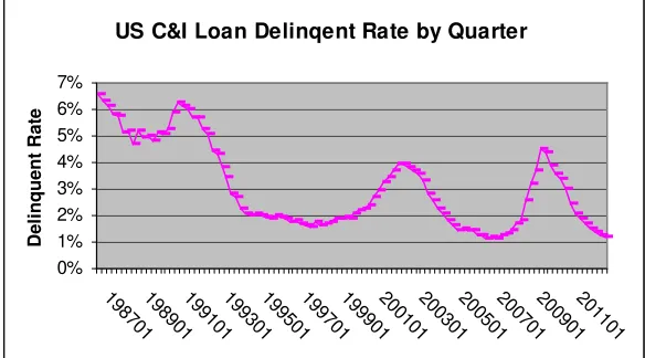
In this section, we estimate the asset correlation, long-run PD for a US commercial portfolio, where historical one-year default rates for the portfolio are available for each quarter between 2006 and 2012.
The market variable we use is the delinquent rate for commercial and industry loans (no seasonal adjustment), posted by US Federal Reserve, available since 1987. The chart below depicts the US delinquency since 1987. There have been two cycles since 1995:
US C&I Loan Delinqent Rate by Quarter
0% 1% 2% 3% 4% 5% 6% 7%
198701198901199101199301199501199701199901200101200301200501200701200901201101
D
e
li
nque
nt
R
a
te
Based on historical default rate data, portfolio default rate responds to US delinquent rate by a lag of two quarters. We thus shift up the US delinquent rate by two quarters to line up with the internal portfolio default rate for modeling purpose.
Again, we follow the steps proposed in section 5 and bootstrap for 1000 times. Each time we fit a type II Vasicek model of the form
p
(
s
)
(
a
bs
1
cs
),
s
~
N
(
0
,
1
)
where 1
(
)
1
US
delinquent
rate
[image:11.612.92.384.359.521.2]s
Table 2 below shows the asset correlation, median/mode PD, and long-run PD by three
approaches. The results show, bootstrap method estimates slightly lower asset correlations, but slightly higher long-run PDs. This is expected as explained in section 5. We calculate the
Table 2. Long-run PD and Asset Correlation on a commercial portfolio using two cycles of US delinquent rates since 199501
Traditional method Bootstrap method
Estimating Median Expected Asset Median Expected Asset
Methodology Avg DR Value PD Value PD Correlation Value PD Value PD Correlation
Binomial 3.01% 2.73% 3.07% 5.16% 2.79% 3.11% 4.7%
Asym Adj 3.01% 2.76% 3.13% 5.34% 2.82% 3.16% 4.9%
Asym 3.01% 2.78% 3.14% 5.81% 2.85% 3.16% 5.3%
Conclusion.
With the proposed Vasicek models for portfolio level PD, asset correlation andlong-run PD for a risk homogenous portfolio both have analytical solutions, parameters can be estimated through least square regression, which is simple and easy to implement. These Vasicek models have the advantages of incorporating longer external market and macroeconomic
variables, improving the quality of parameter estimation in contrast to using only a shorter period of internal default data. The proposed bootstrap approach corrects the bias of parameter estimates by traditional method due to serial correlation. We believe that the proposed models, the
bootstrap technique, and the asymptotic least square approach with a variance correction are potentially a good tool for assessments of long-run PD, asset correlation, and portfolio level PD.
REFERENCES
[1] Basel Committee on Banking Supervision (2005). An Explanatory Note on the Basel II IRB Risk Weight Functions, July 2005.
http://www.bis.org/bcbs/irbriskweight.pdf
[2] Blaschke, W., Jones, M., Majnoni, G., and Peria, S. (2001). Stress Testing of Financial Systems: An Overview of Issues, Methodologies, and FSAP Experiences, IMF working paper, June 2001
[3] Breiman, L. (1996). Bagging Predictors. Machine Learning 24: 123-140
http://www.cs.utsa.edu/~bylander/cs6243/breiman96bagging.pdf
[4] Chernih, A., Vanduffel, S., and Henald, L. (2006). Asset correlations: a literature review and analysis of the impact of dependent loss given defaults
http://www.econ.kuleuven.be/insurance/pdfs/CVH-AssetCorrelations_v12.pdf
[5] Das, S., Duffie, D.,Kapadia, N., Saita, L. (2007) Common Failings: How Corporate Defaults are Correlated. Journal of Finance 62 (1), 93-117
http://www.q-group.org/archives_folder/pdf/Paper-Das.pdf
[6] De Servigny, A., Renault, O. (2003). Default Correlation Evidence. Risk, July 2003, 90-94. [7] Demey, P., Jouanin, J., Roget, C, and Roncalli, T. (2004). Maximum likelihood estimate of default correlations, Risk, November 2004
http://thierry-roncalli.com/download/risk-mledc.pdf
[8] Friedman, J., Hastie, T., and Tibshirani, R. (2008). The Elements of Statistical Learning, 2nd edition, Springer
[9] Frye, J. (2008). Correlation and asset correlation in the structural portfolio model. The Journal of Credit Risk, Volume 4 (2), Summer 2008
http://www.risk.net/digital_assets/4538/v4n2a4.pdf
[10] Gordy, M., Heitfield, E. (2002). Estimating default correlations from short panels of credit rating performance data. Federal Reserve Board Working paper, January 2002 [11] Merton, R. (1974). On the pricing of corporate debt: the risk structure of interest rates. Journal of Finance, Volume 29 (2), 449-470
http://www.jstor.org/discover/10.2307
validation, Volume 3 (3), Fall 2009
http://www.risk.net/digital_assets/5021/jrm_v3n3a3.pdf
[13] Miu, P., Ozdemir, B. (2008). Estimating and validating long-run probability of default with respect to Basel II requirements. The Journal of Risk Model validation, Volume 2/Number 2,
3-41. http://www.risk.net/digital_assets/5008/jrm_v2n2a1.pdf
[14] OSFI (2004). Risk quantification of IRB systems at IRB banks: Appendix – A conservative Estimate of a long-term average PD by a hypothetical bank, December 2004
[15] Pindyck, R. S., Rubinfeld, D. L. (1998). Econometric Models and Economic Forecasts, 4th Edition, Irwin/McGraw-Hill
[16] Rosen, D., Saunders, D. (2009). Analytical methods for hedging systematic credit risk with linear factor portfolios. Journal of Economic Dynamics & Control, 33 (2009), 37-52
http://www.r2-financial.com/wp-content/uploads/2010/07/LinearFactor.pdf
[17] Vasicek, O. (2002). Loan portfolio value. RISK, December 2002, 160 - 162.
[18] Wolfinger, R. (2008). Fitting Nonlinear Mixed Models with the New NLMIXED Procedure.
SAS Institute Inc. http://www.ats.ucla.edu/stat/sas/library/nlmixedsugi.pdf
[19] Zhang, J., Zhu, F., and Lee, J. (2008). Asset Correlation, Realized Default Correlation, and Portfolio Credit Risk, Moody’s KMV, March 2008
http://www.moodysanalytics.com/~/media/Insight/Quantitative- Research/Portfolio-
Modeling/08-03-03-Asset-Correlation-and-Portfolio-Risk.ashx
APPENDIX
Proof of Lemma 2.1. Given s, we have
] 1 / 1 / ) [( ) ( ) ( 2 2 b a b bs P bs a P bs a
where
~
N
(
0
,
1
)
is independent of s. At this moment, s is given as a fixed effect, theonlyrandom variable is
. However, we can view s as random when taking expectation))
(
(
a
bs
E
with respect to s. Sinceu
(
bs
)
/
1
b
2 is standard normal,E
(
(
a
bs
))
is equal to
(
a
/
1
b
2)
.□Proof of Proposition 4.1. We have:
) / ) (( ) / ) ( ( )) ( ( )) ( ( ) ( 1 1 b a w b a w s P y bs a P y z P y p P
where
w
1(
y
)
. The derivative of w with respect to y is given by1
/
(
w
)
. Thus the derivative ofP
(
p
y
)
with respect to y is given by))
(
/(
)
/
)
((
w
a
b
b
w
Replacing w by z, we have statement (a). For (b), if
(
x
)
is the cumulative distribution for a standard normal variable, then the negative log likelihood reduces to
[
1(
)
]
2/(
2
2)
ln(
)
(
1(
))
2/
2
p
b
b
a
p
Proof of Theorem 4.2. By Proposition 4.1 (b), where the parameter b replaces c in Theorem 4.2, the negative log likelihood has the form:
[
(
)]
ln
(
)
(
8
)
2
1
21 1
2
z
a
b
s
N
b
C
z
b
i ikm
i k
N
k
where C(z) depends only on {
z
k}
. With the maximum likelihood approach, parameters areestimated by minimizing (8). Given b, expression (8) is minimized whenever parameters
m
b
b
b
a
,
1,
2,
...,
(which are independent of b) minimize expression (7). For parameter b, taking thederivative of (8) with respect to b and setting the derivative to zero, we have:
2
1 1
2
)]
(
[
1
k i i m
i k
N
k
s
b
a
z
N
b