Rational Expectation Bubbles: Evidence from Hong Kong’s Sub Indices

Munich Personal RePEc Archive

Rational Expectation Bubbles: Evidence

from Hong Kong’s Sub-Indices

Miyakoshi, Tatsuyoshi and Li, Kui-Wai and Shimada, Junji

Hosei University, City University of Hong Kong, Aoyama-Gakuin

University

1 July 2014

Online at

https://mpra.ub.uni-muenchen.de/56118/

Applied Economics, 2014, Vol. 46, Issue 20, pp. 2429-2440

Rational Expectation Bubbles: Evidence from Hong Kong’s Sub-Indices*

Tatsuyoshi Miyakoshia

Hosei University

Kui-Wai Li

City University of Hong Kong

Junji Shimada

Aoyama-Gakuin University

Abstract

This paper uses Hong Kong stock market’s four sub-indices to examine the existence

and causes of rational expectation bubbles. The unit root test is applied to the rational

bubble hypothesis. Various causality test methods are used to examine the causality of

bubble among the four sub-indices. The empirical results show that in the sub-periods

of 1986-2002 and 2000-2012, the bubbles of Commerce & Industry and Utilities

industries are consistent with rational expectation bubbles, but not so in the Finance and Properties industries. In general, the rational expectation bubbles in the two sub-periods seemed to have caused by expectations in other growing foreign economies.

Keywords: rational expectation; stock price bubbles; causality; foreign markets.

JEL Classification Numbers: G12; C50

a

Corresponding author: Tatsuyoshi Miyakoshi, Department of Industrial and System

Engineering, Hosei University, 3-7-2, Kajino-cho, Koganei, Tokyo, 184-8584, Japan.

Tel: 042-387-6352, E-mail: miyakoshi@hosei.ac.jp

* We are grateful to the comments from two anonymous referees and participants, especially Sangho Kim and Frederik Lundtofte, in two conferences (East Asian Economic Association Conference in Singapore in 2012 and 10th Biennial Pacific Rim Conference in 2013 in Tokyo) where the earlier version of this paper was presented. The first author is grateful to research fund provided by the Ministry of Education, Culture, Sport, Science and Technology (Grant-in-Aid 23530367) and the Association of Trust Banks in Japan. The second author is grateful for the research fund from the City University of Hong Kong (Strategic Research Grant numbers 7008129 and 7002532) and Siyang Ye for his research assistance. The authors are solely responsible for the mistakes found in this paper.

I Introduction

Stock market bubble is often defined as the deviation between the stock market price and the fundamental price. The theory of rational expectation bubble in Blanchard and Watson (1982) argued that the movement of stock prices is based on rational expectation, and stock bubbles are characterized by a continuous growth in asset prices caused by opportunistic purchases aimed at securing future capital gains. The theory has aroused interesting debates. For example, Tirole (1982, 1985) showed that stock market speculation relied on “inconsistency plans”. Campbell and Shiller (1987) and Lim and Phoon (1991) showed that stock bubbles are consistent with rational expectation when stock prices and dividends are not cointegrated. By using the Bhargava test to check the robustness of results, Diba and Grossman (1988) concluded that stock prices and

dividends are cointegrated, but argued that stock bubbles reflected a situation of self-confirming divergence of stock prices from market fundamentals in response to

extraneous circumstances. Koustas and Serletis (2005) and Cunado et al. (2005) used a

fractional integration analysis, while Ye et al. (2011) applied a nonparametric rank test

for cointegration on the NYSE or S&P Composite Index.

For a number of reasons, the Hong Kong’s stock market offers an interesting case for the study of stock price. As the third largest world financial center and the freest economy, Hong Kong’s political sovereignty was reverted back to the People’s Republic of China in July 1997 after being a British colony since the end of the Opium War in 1842. Under the constitution described by the Basic Law, Hong Kong becomes a Special Administrative Region that maintains a capitalist system for 50 years under the “one country, two systems” framework. The Hong Kong economy has achieved an advanced status and has been aiding China’s economic reform since 1978. In view of the fact that Hong Kong is a relatively small economy with a quite advanced stock market while China is the largest developing economy with a fast growing but less sophisticated equity market, studies have concentrated on Hong Kong’s financial sector in relation in the growing China economy (Li, 2006, 2012; Schenk, 2009; He et al. 2006, 2009; Leung and Unteroberdoerster, 2008).

Nartea and Wu (2013) pointed that the standard deviation of daily stock market returns in Hong Kong is much higher than that in US in their study from 1992 to 2002. Institutional investors have a weaker role in Hong Kong when compared to the US stock market. Nartea and Wu (2013) also found little support for an idiosyncratic

volatility effect, but other studies pointed to an increasing trend in return idiosyncratic volatility and a ‘puzzling’ negative relationship between idiosyncratic and total

volatility and stock returns. In recent years as shown in Sun et al.(2013), there is a

growing number and concentration of mainland Chinese stocks listed on the Hong Kong stock market in the form of H-share and ‘‘Red Chips’’ (refer as ‘‘China listing’’

hereafter). The increasing presence of mainland Chinese stocks in Hong Kong increases the size, trading volume, and its link with the China and world markets but reduces the overall volatility of the Hong Kong stock market.

One can argue that the Hong Kong stock market fulfilled the conditions in Blanchard and Watson (1982) that rational expectation would occur as a result of unrestricted personal expectation and opportunistic purchases. By using the Hong Kong Hang Seng Index and the US stock market indexes, Lin and Sornette (2013)

demonstrated the feasibility of advance bubble warning to be followed by crashes or

extended market downturns. Ahmed et al. (2010) have examined daily returns of stock

markets in emerging markets including Hong Kong for the absence of nonlinear speculative bubbles. Lehkonen (2010) used the duration test to study Hong Kong’s Hang Seng Index and concluded the absence of rational expectation bubbles.

Most empirical studies on stock markets are based on the general composite index rather than sub-indices that can provide a high data frequency and show the

special characteristics of different industrial and business sectors.In Hong Kong, the

financial sector sub-indices would be volatile and could subject to rational expectation bubble. In the years before and after the hand-over in 1997, for example, Hong Kong has suffered a number of financial crises that have resulted in economic and financial bubbles. Furthermore, the sub-indices on utilities would show a stable performance as utilities consist of non-tradable industries that often served as shelters or “safe havens” in times of financial crises. The manufacturing sector in Hong Kong that once occupied about 30% of GDP in the early 1980s has declined to less than 10% as manufacturing industries have migrated to mainland China (Li, 2012). Such a transition would have reflected in the performance of the industrial sub-indices.

With the use of sub-indices, one can examine whether the performance of particular industries with large increase in their stock price would produce rational expectation bubbles for other industries. It would be useful to test whether the stock price performance of one particular industry could result in the rational expectation

bubble of another industry. In Hong Kong, the composite Hang Seng Index is divided

into four sub-indices of on Utilities, Finance, Properties, and Commerce and Industry.

Using these data and the methodology in Campbell and Shiller (1987), this paper first

applies the ADF and KPSS tests to examine the existence of rational expectation bubble

in Hong Kong’s stock market. This is followed by the use of causality tests in the four

sub-indices. In addition, we hope to provide explanations to the empirical results, as the

four sub-indices would have performed differently.

The paper proceeds as follows. Section II presents the theory, methodology and

the proposition. Section III gives an overview on the statistical performance of the Hong

Kong stock market. The various causality tests on rational expectation bubbles are

conducted in Section IV, while the last section concludes the paper. The measurement

in the difference between the bubble price and the fundamental price in the stock market

based on the study in Miyakoshi et al. (2007) is shown in the Appendix.

II Theoretical Model and Methodology

The definition of rational expectation bubble in Blanchard and Watson (1982) is based on the simple efficient market (no-arbitrage) condition that the expected present value of a stock price at period t is:

(1) 1 1

1

( 1)

t t

t t

t

p d

p E

r

+ + +

 + 

= _{ }

+

 ,

where d_t+1, r_t+1 and E_t[ ]฀ denote, respectively, the dividend, the discount factor (or

stock return) at period t+1 and the expectation conditional on the information set at period t. By calculating the forward infinite periods in Equation (1), the reduced form becomes:

(2)

1 1 1

lim

( 1) ( 1)

t j t j

t t j t _j j

j i t i i t i

d p

p E E

r r

∞

+ +

→∞

= = + = +

   

= _{ }+ _{ }

∏ + _ ∏ + _



∑

 .

Thus, the stock price, p_t, in Equation (2) consists of the fundamental value F_t, which

is defined by the first term in the right hand side, and a bubble price, b_t, which is

defined by the market price minus the fundamental price,p_t −F_t: (3) 1 lim ( 1) t j

t t _j j

i t i p b E r + →∞ = +   ≡ _{ } ∏ +  .

Since the price, b_t, is based on a rational expectation behavior, it is called a rational

expectation bubble. Thus, Equation (2) consists of the fundamental value, F_t, and a

rational expectation bubble, b_t:

(4) p_t = +F_t b_t.

To see how a rational expectation bubble occurs, we insert Equation (4) into

Equation (3) and considering a finiteF_{t+ +j 1}, the first term in the middle becomes zero:

(5)

1 1

lim lim

( 1) ( 1)

t j t j t j

t t _j j t _j j

i t i i t i

F b b

b E E

r r + + + →∞ →∞ = + = + +     = _{ }= _{ } ∏ + ∏ +    .

The b_t on the right hand side of Equation (5) is the solution to a homogeneous

expectation difference equation, given the extraneous price, b_t+1. Then, through an

iteration process, we have:

(6) 1 2

1 1

1 2 1

/( 1) .... lim

1 1 ( 1)

t j

t t

t t t t t t _j j

t t i t i

b

b b

b E E E r E

r r r

+ + + + + _→∞ + + = +         = _{ }= _{  } + _= = _{ } + + ∏ +        .

Thus, as far as people continue to rational expect that the extraneous price, b_t+j, over a

fundamental price rises (for example, at the rate of (r_t+_j +1)), the bubble becomes:

(7)

1

lim 0

( 1)

t j

t t _j j

i t i

p b E r + →∞ = +  

= _{ }>

∏ +

  .

Campbell and Shiller (1989)suggested a log linear approximation of Equation

(1), shown as:

(8) log(1+r_t+1)=log(p_t+1+d_t+1) log(− p_t).

We approximate the left hand side as r_t+1 and the right hand side as:

(9) rt+₁≈ +α λpt+₁+ −(1 λ)dt+₁−pt,

where the tilde letters represent the natural logarithm of a variable, and α and 0 < λ < 1

are parameters.1 Equation (9) is a linear difference equation for the log stock price.

Solving forward and imposing the no rational bubble terminal condition, we have:

(10) lim j t j 0

j→∞λ p+ = , and obtain:

(11)

0 [(1 ) ]

1

j

t _j t j t j

p α λ λ d r

λ

∞

+ + =

= + − −

−

∑



 .

Finally, taking the mathematical expectation of Equation (11) based on the information available at time t and rearranging in terms of the log dividend–price ratio yields:

(12)

0 [ ]

1

j

t t t _j t j t j

d p α E λ d r

λ

∞

+ + =

 

− = − + _ −∆ + _

−

∑

 _  _.

Campbell and Shiller (1989) have derived the necessary condition for non-rational expectation bubble that the log dividend and log stock price have

cointegrating vector restricted to (1, -1), namely, the log dividend yield,d_t− p_t, is

stationary, if rational expectation bubbles do not exist. Craine (1993) pointed out that if

the dividend growth factor, ∆d_t+j and the stock returns, r_t+j, are stationary stochastic

processes, then the log dividend yield,d_t −p_t, is a stationary stochastic process under

the no rational bubble restriction. On the contrary, the presence of a unit root in the log dividend yield is consistent with rational expectation bubble in stock prices. Taking

contraposition from the Campbell and Shiller (1989) proposition, we can derive the

1 _{Note that for the discount factor,}

1

t

r₊ , Campbell and Shiller (1989, p. 203) used the rate of treasury bill, commercial paper and stock index return. The stock index return is used here.

sufficient condition for the rational expectation bubbles as follows.

Proposition 1:Suppose that the dividend growth factor, ∆d_t and the stock returns, r , _t

are stationary stochastic processes,rational expectation bubbles exist if the log

dividend yield,d_t −p_tis not stationary.

III Data and Performance in Hong Kong’s Stock Price

The monthly data of Hang Seng Index (HSI) and the four sub-indices (Finance, Properties, Utilities, and Commerce & Industry) are compiled from Datastream for the period from 1986:01 to 2012:08. Figure 1 plots the logged market prices and the fundamental prices of the four sub-indices. The computation method for the fundamental price is described in Appendix. As Figure 1 shows, Hong Kong’s

composite HSI exhibits a number of setbacks during the sample period. Firstly, the fall

in 1989 was probably due to the June 4th Tiananmen incident in Beijing, and economic

pessimism persisted until recovery in 1992 after the late Deng Xiaoping reasserted

economic reform in his spring visit to Shenzhen.The setback in 1995 was short-lived

and responded to the ultra-rapid rise in income and wealth prior to the 1997 sovereignty

change.

The Hong Kong economy recessed for a couple of years in the mid-1980s

during the Sino-British negotiation over the post-1997 political future of Hong Kong.

By late 1980s, the economy recovered and began to experience overheating in the early

1990s, as inflow of hot money took advantage of the 1997 sovereignty reversion and

widespread speculation in stocks and property emerged. In the meantime, the low cost

provision in the China economy had gradually attracted industrial investments from

Hong Kong, and manufacturing began to migrate, leading to a fall in manufacturing

output and domestic export.

However, after the burst of the Asian financial crisis in 1997-1998, the

prolonged economic recession reflected the shrinking industrial structure as Hong

Kong’s industrial capacity and economy was too weak to sustain the collapsing stock

market. While the Asian financial crisis was more of a regional crisis, the dotcom

bubble in 2000-2001 was global and had imposed another setback to the stock market in

Hong Kong. Although the stock market recovered by 2001, the outbreak of the severe

acute respiratory syndrome (SARS) led to another downfall in 2003-2004. While the

Hong Kong economy stabilized by 2005, the U.S. financial crisis in 2008 was another

crisis that led to a sharp fall of the stock price. Li (2013) concluded that the first decade

of the Hong Kong economy after sovereignty change in 1997 has suffered from periodic

crises, economic recession and a young government.

Besides exogenous shocks, there were also institutional changes in the Hong

Kong stock market itself and the impact of listing deregulation in mainland China that

affected the Hong Kong market from 1986-2012. Sun et al (2013, p. 2230) pointed out:

the so-called ‘‘through-train program’’ suggested by the State Administration of Foreign Exchange (SAFE) in August 2007 under which mainland individuals are allowed to buy Hong Kong stocks directly. The announcement brought the Hang Seng China Enterprises Index, which represented the H-shares, up by 68.8% and the HSI up by 60% in 3 months even though the subprime mortgage crisis began to surface. However, the program was shelved by Premier Wen Jiabao when he expressed his worries on the program in November 2007. Subsequently, the HSI plummeted by 10,000 points from its record high of 32,000 in October 2007 to 22,000 in January

2008.2

One can see from the four sub-indices that the gaps between the logged market

price and the logged fundamental price are narrower in both Utilities and Finance

sub-indices. The Finance sub-index shows a close movement with the composite HSI,

but despite its volatility, the Finance sub-index tends to have fluctuated less drastically

than both Properties and Commerce & Industry. The Properties sub-index has shown a

wide gap between the market price and fundamental price, especially after the early

1990s, indicating widespread speculation in properties. Indeed, the “short-term

investment behavior” appeared in the transition years prior to 1997 (Li, 2006, 2012) has

resulted in speculation. The inflow of “hot money” prior to 1997 had pushed up

property price severely. The Commerce & Industry sub-index has also shown a big gap

between the two prices, but it also dropped severely in 1998 during the Asian financial

2 _{The program was allowed to proceed in 2012.}

crisis and in 2003 at the outbreak of SARS. While the commerce sector contains mainly

business services, their economic performance has been highly vulnerable to economic

shocks. Manufacturing in Hong Kong has been weakened as many manufacturing

industries have moved to southern China since the late 1980s when low wages and

attractive government policies across the border appeared.

The monthly Hong Kong data contain both the stock price and dividend yield for each of the four categories. The dividend yield data are used as a proxy for

dividends. The dividend yield for each category is defined as the “total dividend of index constituent stocks divided by the index market capitalization”. This is equivalent to say that the dividend is divided by stock price index. We can proxy the dividend by using the product of “dividend yield” and “stock price index” (Hang Seng Bank, 2012).

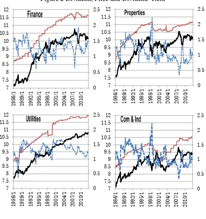
Figure 2 plots the logarithms of the price, dividend, and dividend yield of the four sub-indices. The log of the dividend yield is presented on the right hand side of the vertical axis. There is no apparent trend in the log of the dividend yield during the sample period. For the two sectors of Finance and Properties, they look like mean reverting (stationary), but otherwise (non-stationary) for the two sectors of Commerce & Industry and Utilities. This supports the fact that the stock prices for the two sectors of Commerce & Industry and Utilities are consistent with a rational expectation bubble.

[image:11.595.86.500.146.745.2]

Figure 1 Hong Kong’s Monthly Stock Price Indexes

7.0 7.5 8.0 8.5 9.0 9.5 10.0 10.5 11.0 19 86 /1 19 89 /1 19 92 /1 19 95 /1 19 98 /1 20 01 /1 20 04 /1 20 07 /1 20 10 /1

Hang Seng Index

7.0 7.5 8.0 8.5 9.0 9.5 10.0 10.5 11.0 19 86 /1 19 89 /1 19 92 /1 19 95 /1 19 98 /1 20 01 /1 20 04 /1 20 07 /1 20 10 /1 Utilities 7.0 7.5 8.0 8.5 9.0 9.5 10.0 10.5 11.0 19 86 /1 19 89 /1 19 92 /1 19 95 /1 19 98 /1 20 01 /1 20 04 /1 20 07 /1 20 10 /1 Finance 7.0 7.5 8.0 8.5 9.0 9.5 10.0 10.5 11.0 19 86 /1 19 89 /1 19 92 /1 19 95 /1 19 98 /1 20 01 /1 20 04 /1 20 07 /1 20 10 /1 Properties 7.0 7.5 8.0 8.5 9.0 9.5 10.0 10.5 11.0 19 86 /1 19 89 /1 19 92 /1 19 95 /1 19 98 /1 20 01 /1 20 04 /1 20 07 /1 20 10 /1 Com&Ind

Logged Market Price

Logged Fundamental Price

[image:12.595.88.506.111.556.2]

Figure 2 Dividend, Price and Dividend-Yield

0 0.5 1 1.5 2 2.5 7 7.5 8 8.5 9 9.5 10 10.5 11 11.5 12 19 86/ 1 19 89/ 1 19 92/ 1 19 95/ 1 19 98/ 1 20 01/ 1 20 04/ 1 20 07/ 1 20 10/ 1 0 0.5 1 1.5 2 2.5 7 7.5 8 8.5 9 9.5 10 10.5 11 11.5 12 19 86/ 1 19 89/ 1 19 92/ 1 19 95/ 1 19 98/ 1 20 01/ 1 20 04/ 1 20 07/ 1 20 10/ 1 0 0.5 1 1.5 2 2.5 7 7.5 8 8.5 9 9.5 10 10.5 11 11.5 12 19 86/ 1 19 89/ 1 19 92/ 1 19 95/ 1 19 98/ 1 20 01/ 1 20 04/ 1 20 07/ 1 20 10/ 1 0 0.5 1 1.5 2 2.5 7 7.5 8 8.5 9 9.5 10 10.5 11 11.5 12 19 86/ 1 19 89/ 1 19 92/ 1 19 95/ 1 19 98/ 1 20 01/ 1 20 04/ 1 20 07/ 1 20 10/ 1 Logged Price Logged Dividend

Logged Dividend-Yield (right hand axis)

IV Statistical Tests for Rational Expectation Bubbles

We will test whether the sub-indices are consistent with a rational expectation bubble. The sample period is divided into two sub-periods of 1986:1-2002:3 and 2000:4-2012:8. The first period includes the consequences of the Asian financial crisis, which is mainly a regional crisis. The second period covers the situation of the global dotcom bubble in 2000 and the US financial in 2008. The two sub-periods thus provide analysis on both the regional financial crisis and the two global crises in 2000 and 2008.

IV.1 Tests of the Assumptions

The assumptions in Proposition 1 that the dividend growth factor, ∆d_t and the

stock returns, r_t, are stationary stochastic processes, are confirmed by the test results

shown in Table 1. Columns 2–4 in Table 1 report the t-statistics for the augmented Dickey–Fuller (ADF) test with the null hypothesis of a unit root (Dickey and Fuller, 1979). The reported t-statistics are based on the regressions with the following

deterministic components: no deterministic components,

τ

, a constant only, τ_µ , and

a constant and a linear trend, τ_τ . The procedure for choosing the optimal lag length is

to test between one-lag and twenty four-lag for the AR, by using the minimum value of the Akaike Information Criterion (AIC). The residuals from the chosen AR are then

checked for whiteness.3 If the residuals in any equation proved to be non-white, we

sequentially chose a higher lag structure until they are whitened. The optimal lag lengths are reported in columns 5–7 of Table 1. The ADF test rejects entirely the

unit-root null hypothesis for the dividend growth ∆d_t and the market return r_t in the

assumptions of Proposition 1.

3 _{Following Gonzalo (1994), the whiteness is checked by the Ljung-Box Q tests for} absence of correlation for all 24 (or 18) lags at 5% significance level.

[image:14.595.77.506.130.537.2]

Table 1 Tests of Stationarity for ∆d_tand r_t

Variable ADF AIC lags KPSS

τ τµ ττ ηµ ητ

1986:1-2002:3

Finance △dt -1.357 -3.481 -3.451 13 12 12 0.147 0.121

rt -9.784 -10.131 -10.126 1 1 1 0.075 0.058

Properties △dt -3.993 -4.308 -5.514 5 5 5 1.398 0.049

rt -8.724 -8.826 -8.937 2 2 2 0.157 0.025

Com&Ind △dt -2.588 -2.583 -9.064 11 11 4 0.749 0.039

rt -8.366 -8.400 -8.498 2 2 2 0.179 0.035

Utilities △dt -9.191 -9.653 -9.627 1 1 1 0.035 0.034

rt -10.55 -11.009 -10.993 1 1 1 0.036 0.029

2000:4-2012:8

Finance △dt _{-8.465 -8.540 -8.610 1 1 1 0.169 0.033}

rt -8.053 -8.037 -8.048 1 1 1 0.251 0.034

Properties △dt _{-9.981 -8.085 -8.101 1 3 3 0.077 0.038}

rt -9.403 -9.381 -9.357 1 1 1 0.053 0.047

Com&Ind △dt -8.465 -8.540 -8.610 1 1 1 0.169 0.033

rt -8.420 -8.392 -8.509 1 1 1 0.329 0.179

Utilities △dt -7.277 -7.690 -7.269 5 5 8 0.051 0.047

rt -6.149 -9.142 -9.134 2 1 1 0.062 0.033

Critical value 0.05 -1.942 -2.881 -3.440 0.463 0.146

Notes: The null hypothesis in the ADF test is the unit root, while the null hypothesis in the KPSS test is stationarity. The numbers in the columns for ADF and KPSS are test statistics and the critical values at 5% significance level are shown at the bottom of the

table. The optimal lag length for AIC lags, are shown respectively for

τ τ τ

, _µ, _τ. The

reported KPSS statistics are based on the same lag-length as those of ADF test.

The Kwiatkowski-Phillips-Schmidt-Shin test (KPSS) (Kwiatkowski et al. 1992)

argued that unit-root tests often fail to reject a unit root because they have low power against relevant alternatives, and proposed that the KPSS test for the null hypothesis of stationarity, as this can complement the unit-root tests. The KPSS test statistics,

reported in columns 8 and 9 of Table 1, cannot reject the null hypotheses of level and

trend stationarity. Combining the results of the two tests, we conclude that the

assumptions are satisfied in Proposition 1, and that the dividend growth factor, ∆d_t

[image:15.595.80.508.248.494.2]

and the stock returns, r_t, are stationary stochastic processes.

Table 2 Tests for Stationarity of Logged Dividend-Yield, d_t −p_t

Variable ADF AIC lags KPSS

τ τµ ττ ηµ ητ

1986:1-2002:3

Finance Properties

Commerce & Industry Utilities

-0.562 -0.668 -1.043 -0.013

-3.092 -3.604 -2.128 -2.596

-3.204 -3.891 -3.214 -2.892

1 4 4 1

1 1 10 1

1 1 10 1

2.719 1.376 0.880 1.575

0.675 0.433 0.180 0.439

2000:4-2012:8

Finance -0.201 -3.398 -3.386 1 3 3 0.127 0.108

Properties -0.555 -3.259 -3.469 1 1 1 1.246 0.338

Commerce & Industry -0.139 -2.174 -2.835 6 6 6 1.146 0.228

Utilities -1.243 -1.604 -3.237 6 1 2 6.104 0.122

Critical values 0.05 -1.942 -2.881 -3.440 0.463 0.146

Notes: Same as Table 1.

IV.2 Tests for Rational Expectation Bubbles

In Table 2, we perform the ADF test and KPSS test against the sufficient condition, namely the log dividend yield is not stationary, for existence of rational expectation bubbles in Proposition 1. Combining both test results, we conclude that the

log dividend yield, d_t− p_t, for the Commerce & Industry and Utilities industries are

not stationary, supporting the existence of rational expectation bubbles for the Utilities and Commerce & Industry sectors in the two sub-periods of 1986:1-2002:3 and 2000:4-2012:8. However, the two sectors of Finance and Properties are not consistent with the rational expectation bubble. The only exception is found in the no deterministic

components, τ . However, as seen in Figure 2, there exists obviously deterministic components (constant term in the test regression) for the log dividend yield. In spite of deterministic components, we have to test for no deterministic components.

As argued in Diba and Grossman (1988), a specific sector that experienced a large increase in its stock price could induce the expectation for the economy to growth further and would produce a rational expectation bubble in other industries. This argument can be tested by using the performance of the four sub-indices in the Hong Kong stock market to see if there were rational expectation bubbles. In particular, we would investigate if the rational expectation bubbles in the two sectors of Utilities and Commerce & Industry are caused by either the two growth-leading industries

(Properties and Finance) in Hong Kong or by the impact from foreign markets. As pointed out earlier, the stock price in the Utilities often served as “safe havens”, while manufacturing industries in Hong Kong has been shrinking as many industrialists have moved their plants across the border to south China beginning from the mid-1980s.

We first conduct the causality tests among the stock returns r_t of all

sub-indices (Sims, 1972, Geweke et al., 1983, Granger, 1969). Considering the unit root

test results shown in Table 1, we see that the stock returns are stationary, and we can then use these tests directly with the ad hoc lag length of 12. For the Sims (1972) test, we pre-filter the variables with (1 - 0.75L) and compute a two-sided distributed lag of

stock return r_u of Utilities (u) on Finance (f), r_f, and then test the leads

0 ( 6,.. 1)

i

b = i= − − of Utilities (u):

(13) _, 12 _{, 0}

6 , : 0 ( 6,.. 1);

f t _i i u t i t i f u

r a b r ε H b i r r

× −

=−

= +

∑

+ = = − − → ,

where 2

(0, )

t N

ε ฀ σ is a stochastic term and a is a constant term.

To conduct the test in Geweke et al. (1983), we further include the lag of the

Finance industry in Equation (13):

(14) _, 12 _, 12 _{, 0}

6 1 , : 0 ( 6,.. 1);

f t _i i u t i _i i f t i t i f u

r a b r c r ε H b i r r

×

− −

=− =

= +

∑

+

∑

+ = = − − → .

To conduct the Granger (1969) test, we regress the stock return r_u of Utilities (u) on

lags of Finance (f) and Utilities (u):

(15) _, 12 _, 12 _{, 0}

1 1 , : 0 ( 1,.,12);

u t i i u t i i i f t i t i f u

r a b r c r ε H c i r r

×

− −

= =

= +

∑

+

∑

+ = = → .

Table 3 shows all the causality test results in a bivariate model. The figures in the columns in Table 3 denote the significance level for the null hypotheses in Equations (13)-(15). On the contrary, the significance levels for non-causality are shown from the figures in the rows to figures in the columns. For example, in Table 3 (1986:1-2002:3), the significance level for non-causality from Finance returns to Properties returns is 0.311. In the first sub-period (1986-2002) that covered the influence of the Sino-British negotiation over the future of Hong Kong in 1982-1984 and the impact of the Asian financial crisis in 1997-1998, the rational expectation stock bubbles were not

indigenously caused by industries within Hong Kong. However, one can see that the stock bubbles in the two sectors of Utilities and Commerce & Industry were caused by the impact from other world financial markets and/or the impact from the growing world economy. In the second sub-period (2000-2012) that covered the influence of the dotcom bubble in 2000 and the US crisis in 2008, the rational expectation bubble of the Utilities was caused by the other domestic industries that contributed to Hong Kong’s economic growth. However, the rational expectation bubble of the Commerce & Industry was not caused by the impact from other domestic industries, but was caused by impact from the growing world economy.

IV.3 Robustness Checks

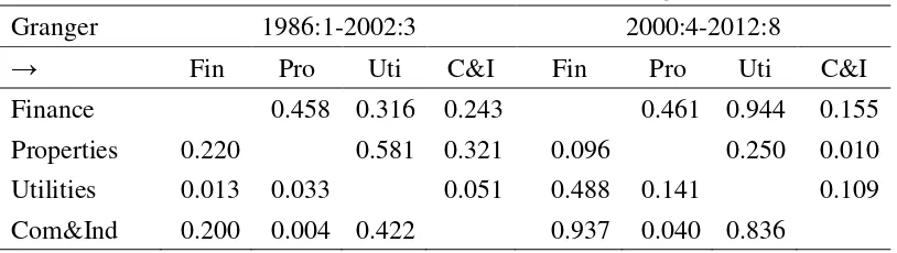
We check the robustness of the results in Table 3 by using the multivariate generalization of Granger causality in the framework of VAR model. We chose the 6 lag-length for each variable which equals to the total lagged variables in Equation (15).

(16)

6

, , , , ,

1

0 ,

: [ ]; ( , , , ) ; (0, )

. : 0 ( 1,., 6);

t _i i t i t i h k i t f t p t u t c t t

fu i f u

Y a C Y C c Y r r r r N

Eg H c i r r

ε ε

− =

×

′

= + + = = Σ

= = →

∑

฀

Table 4 shows the results of causality. Most of the results support the robustness, except for the Utilities in the second sub-period (2000-2012). We thus have to suspend the result for the Utilities industry.

[image:18.595.81.490.136.474.2]

Table 3 Stock Returns Exogeneity

Sims 1986:1-2002:3 2000:4-2012:8

→ Fin Pro Uti C&I Fin Pro Uti C&I

Finance 0.311 0.460 0.118 0.085 0.027 0.233

Properties 0.342 0.786 0.061 0.003 0.006 0.024

Utilities 0.046 0.213 0.038 0.691 0.836 0.556

Com&Ind 0.446 0.068 0.330 0.156 0.001 0.003

GMD 1986:1-2002:3 2000:4-2012:8

→ Fin Pro Uti C&I Fin Pro Uti C&I

Finance 0.438 0.554 0.185 0.140 0.000 0.073

Properties 0.404 0.804 0.118 0.023 0.000 0.006

Utilities 0.078 0.311 0.104 0.556 0.602 0.164

Com&Ind 0.566 0.042 0.154 0.200 0.000 0.013

Granger 1986:1-2002:3 2000:4-2012:8

→ Fin Pro Uti C&I Fin Pro Uti C&I

Finance 0.706 0.147 0.353 0.050 0.002 0.218

Properties 0.850 0.392 0.106 0.029 0.010 0.153

Utilities 0.244 0.251 0.115 0.102 0.033 0.088

Com&Ind 0.913 0.170 0.148 0.078 0.003 0.024

Notes: The figures in the columns denote the significance level of the null hypotheses in Equations (13)-(15). The significance level for non-causality for variables can be read

from the rows to the columns. Geweke et al. (1983)’s test is denoted as GMD.

Table 4 Multivariate Generalization of the Granger Causality

Granger 1986:1-2002:3 2000:4-2012:8

→ Fin Pro Uti C&I Fin Pro Uti C&I

Finance 0.458 0.316 0.243 0.461 0.944 0.155

Properties 0.220 0.581 0.321 0.096 0.250 0.010

Utilities 0.013 0.033 0.051 0.488 0.141 0.109

Com&Ind 0.200 0.004 0.422 0.937 0.040 0.836

Note: The figures in the columns denote the significance level of the null hypotheses.

[image:18.595.80.487.581.696.2]

IV.4 Discussion on Real Estate Bubble and Externally-imposed Monetary Policy Is there any relationship between stock market bubbles and bubbles in other assets, particularly real estate prices? The movement of the Properties and other sub-indices seem to closely track the returns from outright ownership of property. On the other hand, what role does the exchange rate regime play in the emergence of bubbles? Hong Kong has a currency board arrangement that prevents the interest rate diverging from the US rate. This limits pre-emptive action, and bubbles seem to arise when US monetary policy is particularly loose.

We use a 5-dimensional VAR model to examine the relationship between stock price bubble, real estate bubble and the US interest rate. The US call money rate data come from the OECD Database, while the Hong Kong real estate price data come from

Rating and Valuation Department, Hong Kong SAR.4 As shown in Table 4, we chose

the 4 lag-length for the five variables including monthly real estate price return,r_{r t,} , and

incorporate one exogenous variable of the first difference of the logged US monthly call

rate, ϕ_t.5 We chose the 4 lag-length for each variable which equals to the total lagged

variables in Equation (15).

(17)

4 4

1 1

, , , , ,

, , , , ,

0 ,

: ~ (0, )

( , , , , ) , [ ], ,

( , , , , )

. : 0 ( 1,., 4);

t i i t i i i t i t t

t f t p t u t c t r t i hk

i f i p i u i c i r i

f u i f u

Y a C Y Id N

where Y r r r r r C c I identity matrix

and d d d d d d

Eg H c i r r

ϕ ε ε

− −

= =

×

= + + + Σ

′

= = =

=

= = →

∑

∑

We introduce an exogenous variable of ϕ_tfor system (17). Then, we have to test

whether ϕ_t affect the variable Y_t, i.e., whether we should introduce the US monthly

call rate into system (17). By using the Likelihood Ratio, we test the null hypothesis of no effects on system (17) by the US monthly call rate. In Table 5, we can find the

4 _{The real estate price includes monthly, quarterly and annual data. But the monthly}

data starts from 1993M1. Then, we got the monthly data from 1986M1 to 1992M12 by using linear interpolation on quarterly data.

5 _{We have implemented an ADF test for the first difference of the logged US monthly}

of the call rate and for the first difference of the logged real estate price as well as in

Table 1. The results are that all are stationary for both periods. However, the level US call rates have unit roots for both periods even by using ADF test without constant term and trend, with constant term, with constant term and trend.

significance level for null hypothesis, 0.077 for the first period and 0.89 for the second period. Thus, we need not to introduce the US monthly call into system (17). Without the US call, our estimate shown in Table 5 confirm that the results in Table 4 are robust; that is, the rational expectation bubble of the Commerce & Industry and the Utilities in both sub-periods was not caused by the impact from other domestic industries, but was caused by impact from the growing world economy.

In short, the Hong Kong stock market presents an ideal setting for the

[image:20.595.77.523.453.604.2]

investigation on the rational expectation bubble. On the other hand, Hong Kong has a currency board arrangement that prevents the interest rate diverging from the US rate, though this policy imposed no significant impact in our results. Moreover, the Hong Kong has shortage of land, and returns from outright ownership of property attracted investors. However, the real estate bubbles have no effects on the other bubbles in the two sub-periods, as shown in Table 5. Rather, the impact of the real estate bubble came from the bubbles occurred in other industries, especially in the first sub-period.

Table 5 Multivariate Generalization of the Granger Causality with Real Estate

Granger 1986:1-2002:3 2000:4-2012:8

→ Fin Pro Uti C&I Real Fin Pro Uti C&I Real

Finance 0.329 0.658 0.171 0.037 0.342 0.823 0.269 0.639

Properties 0.220 0.518 0.209 0.013 0.093 0.357 0.015 0.092

Utilities 0.012 0.017 0.073 0.028 0.565 0.864 0.511 0.041

Com&Ind 0.331 0.002 0.151 0.002 0.882 0.001 0.945 0.135

RealE 0.498 0.698 0.267 0.510 0.892 0.476 0.615 0.592

UScall 29.589 (0.077) 12.677 (0.89)

Note: The “UScall” means the US call rate, where the figure in the column denote

Chi-squared (χ2₎

and the figure in parenthesis is significance level for null hypothesis. The “RealE“ means the real estate price’s return. The figures in the columns denote the significance level of the null hypotheses of non-causality without the US monthly call rate.

V Conclusion

By using the data from Hong Kong’s four sub-indices, we conducted the unit root test on the existence of rational bubble, and in turn the causality of bubble is examined by several causality test methods. The first finding is that in the two sub-periods of 1986-2002 and 2000-2012, the Commerce & Industry and Utilities

industries are consistent with rational expectation bubbles, while those of the Finance and Properties are not. Secondly, the rational expectation bubble of the Utilities in the second sub-period (2000-2012) was caused by the other three industry sectors that reflected the growing Hong Kong economy, while that of the Commerce & Industry sector was caused by the industries in foreign countries. However, we cannot confirm the robustness of the result of Utilities. Rather, when we introduce the real estate price bubble (not stock price bubble for real estate industry) into the estimation model, the rational expectation bubble of the Commerce & Industry and the Utilities in the two sub-periods was not caused by the impact from other domestic industries, but was caused by impact from the growing world economy. Thirdly, Hong Kong’s conspicuous elements for research phenomena are the real estate bubble and the externally-imposed monetary policy (depending on US monetary policy). The latter element did not affect our results. The real estate bubble did not affect the bubbles of other industry but were affected from the others.

These results suggest that studies using sub-indices can show the performance of different industries, and that different bubbles can be distinguished so that different policies would be needed to deal with the industries. Diba and Grossman (1988) argued that rational expectation is caused by the growing foreign economy. Even recent studies

such Koustas and Serletis (2005), Cunado et al. (2005) and Ye et al. (2011) have not

derived uniform evidence for rational expectation bubble. However, using sub-indices and the Hong Kong market as an ideal setting for the investigation on the rational expectation bubble, as in Lam and Tam (2011), Nartea and Wu (2013),

Lin and Sornette (2013) and Ahmed et al., (2010), we have derived a positive evidence

for rational expectation bubble.

If domestic policies were necessary, Diba and Grossman (1988) proposed to implement individual industry policies against the non-rational expectation bubbles. As such, these results also supported the needed theories for the study of non-rational

expectation bubble in the Hong Kong stock price. For example, Guo and Hung (2010)

incorporated the inflow of hot money in their analysis, while Wang et al. (2011)

focused on stronger integration in the global financial market, and Koivu (2012)

examined the relevance of monetary policy in China’s stock market. As shown in Li and Kwok (2009) and Li (2006, 2012), the finance sector in Hong Kong is international and

that its market movements would have followed that in other world financial centers.

The “short-term investment behavior” that appeared in Hong Kong’s transition years

prior to 1997 would have resulted in speculation, and the inflow of “hot money” had

pushed up property price severely.

Appendix: Measuring Bubble Prices

Miyakoshi et al. (2007) proposed the following methodology to measure the

stock price bubble within the framework of Blanchard and Watson (1982). Suppose that

people expect at time t the present dividend growth rate λ_t and the discount rate r_t

will continue. Then, people expect the dividend grows at a constant rate λ_t from t,

namely d_{t, j}=d_t(1+λ_t)j for all period j and for an initial value of d_t. The fundamental

value F_t in Equations (2) and (4) is expressed as:

(A1) ₁ 1

0 1 1 1

(1 ) 1

( 1) (1 )

j

t t t

t j

t t j j t

j i t i j t t t

d d

F E d

r r r

λ λ

λ

∞ ∞

+ + +

= = + − =

 

+ +

 

≡  _{∏ +} = ₊ = _{ −} _



∑



∑

  ,

where r_t >λ_t is assumed. Considering Equation (A1), the growth rate η_t of the

fundamental value is shown as:

(A2)

1 1 1 1

1 1 1 1 1

1 1

1 1 1 1

1 1

t t t t t t t t t

t

t t t t t t t t t

F d r d r

where

F d r d r

λ λ λ λ

η

λ − λ− λ − λ−

− − − − −

+ − + −

≡ − = − = − ≈

+ − + − .

Then, the growth rate of the fundamental value equals the growth rate of dividend,

t t

η =λ . Given F_t−1, we can compute the fundamental value F_t as:

(A3) _{1 0}

0

(1 ) (1 )

t

t t t t j

j

F F₋ λ or F F λ

=

= + =

Π

+ .

The market price for a stock is said to be overvalued (bubbled) if

P

t

>

F

t in Equation

(A3),undervalued if

<

P

t

F

t , and normal otherwise.

However, F₀ is unknown in practice. Therefore, we use the following method to

identify the unknown F₀ . Suppose F₀ =P₀ for a particular month and we compute

the path of F₀−_j for some j. When the following condition holds,

(A4) F0−j(1 0.05)− ≤P0−j ≤F0−j(1 0.05 ) for some duration of j+ ,

we define that at period 0, F₀ =P₀ , and also that the price P_0−j is not overvalued nor

undervalued until period 0. Some duration in Equation (A4) is needed in this definition because the market price normally equals to the fundamental price. Then, at least, the growth rate of the fundamental value must be roughly equal to that of the market price

until period 0 from several past periods. When the following condition holds,

(A5) F₀ t(1 0.05) P₀ t for all t from T to T ,

∗ ∗∗ + + < +

we define the stock price P_t as being overvalued from T* to T**. The size of the

bubble is defined as P_0+t−F_0+t.

We depict the figure for the market price, the fundamental prices and the size of bubble based on Equations (A4)-(A5). The Hong Kong data in January 1990 showed

that F₀ =P₀ , and this satisfied the condition in Equation (A3). We also recognized that

the price P_0−j is neither overvalued nor undervalued for several years before January

1990. The bubbles in all four sectors can explicitly be seen from February 1990 onwards, as shown in Figure 1. However, the bubbled prices (the size of bubbles) for Utilities and Commerce & Industry continue to go up and down (large and small). That is to say, the bubbled prices seemed to react to the rapidly growing economy of Hong Kong or the other economies. On the other hand, the bubbled prices for Finance in particular and Properties increased rapidly around the time of the dotcom bubble and the global financial crisis bubble, but disappeared afterwards.

References

Ahmed, E., Rosser, B. and Uppal, J.Y. (2010), ”Emerging markets and stock market

bubbles: Nonlinear speculation?”, Emerging Markets Finance and Trade ,

46: 23–40.

Blanchard, O. and Watson, M. W. (1982), Bubbles, Rational Expectation and Financial

Markets, No. 9115,NBER Working Paper Series.

Craine, R. (1993),”Rational bubbles”, Journal of Economic Dynamics and Control, 17: 829-846.

Campbell, J. Y. and Shiller, R. J. (1987), “Cointegration and tests of present value

models”, Journal of Political Economy, 95: 1062–1088.

Campbell, J. Y. and Shiller, R. J. (1989), “The dividend-price ratio and expectations of

future dividends and discount factors”, Review of Financial Studies, 1:

195-228.

Cuñado, J., Gil-Alana, L. A. and Perez de Gracia, F. (2005), “A test for rational bubbles

in the NASDAQ stock index: A fractionally integrated approach”, Journal of

Banking & Finance, 29: 2633−2654.

Diba, B.T. and Grossman, H. (1988), “Explosive rational bubbles in stock prices?”,

American Economic Review, 78: 520-530.

Dickey, D. A. and W. A. Fuller (1979), “Distribution of the estimators for

autoregressive time series with a unit root”, Journal of the American Statistical

Association, 74: 427-431.

Geweke, J., Meese, R. and Dent, W. (1983), “Comparing alternative tests of causality

in temporal systems”, Journal of Econometrics, 21: 161-194.

Gonzalo, J. (1994), “Five alternative methods of estimating long-run equilibrium

relationships”, Journal of Econometrics, 60:203-233.

Granger, C. W. J. (1969), “Investing causal relations by econometric models and cross

spectral methods”, Econometrica, 37: 424-438.

Guo, F. and Huang, Y. S. (2010), “Does “hot money” drive China's real estate and stock

markets?”, International Review of Economics and Finance, 19: 452–466.

Hang Seng Bank, (2012), Index Operation Guide, Version 2.1, July: 19.

He, D., Young, I. and Lim, P. (2006), “Financial sector output and employment in Hong

Kong and New York city”, Hong Kong Monetary Authority Quarterly Bulletin,

22-29.

He, D., Zhang, Z. and Wang, H. (2009), Hong Kong’s Financial Market Interactions

with the US and Mainland China in Crisis and Tranquil Times, Working Paper

10/2009, Hong Kong Monetary Authority, June.

Koivu, T.(2012), “Monetary policy, asset prices and consumption in China”, Economic

Systems, 36: 307–325

Koustas, Z. and Serletis, A. (2005), “Rational bubbles or persistent deviations from

market fundamentals?”, Journal of Banking & Finance, 29: 2523–2539.

Kwiatkowski, D., Phillips, P. C. B., Schmidt, P. and Shin, Y. (1992), “Testing the null

hypothesis of stationarity against the alternative of a unit root”, Journal of

Econometrics, 54: 159-178.

Lam, K. S. K. and Tam, L. H. K. (2011), Liquidity and asset pricing: Evidence from

the Hong Kong stock market, Journal of Banking and Finance ,35: 2217-2230.

Lehkonen, H. (2010), “Bubbles in China”, International Review of Financial Analysis,

19: 113–117.

Leung, C. and Unteroberdoerster, O. (2008), Hong Kong SAR as a Financial Center in

Asia: Trends and Implications, Working Paper WP/08/57, Asia and Pacific

Department, International Monetary Fund, Washing DC, March.

Li, K.-W. (2006), The Hong Kong Economy: Recovery and Restructuring, McGraw

Hill Educational (Asia), Singapore.

Li, K.-W. (2012), Economic Freedom: Lessons of Hong Kong, World Scientific,

Singapore.

Li, K.-W. and Kwok, M.-L. (2009), “Output volatility of five crisis-affected East Asia

economies", Japan and the World Economy, 21 (2): 172-182.

Lim, K. G. and Phoon, K. H. (1991), “Tests of rational bubbles by using cointegration

theory”, Applied Financial Economics, 1: 85-87.

Lin, L. and Sornette, D. (2013), Diagnostics of rational expectation financial bubbles

with stochastic mean-reverting termination times, European Journal of

Finance , 19: 344-365.

McQueen, G. and Thorley, S. (1994), “Bubbles, stock returns, and duration

dependence”, Journal of Financial and Quantitative Analysis, 29: 379-401.

Miyakoshi, T, Tsukuda, Y. and Shimada, J. (2007), Market Efficiency, Asymmetric

Price Adjustment and Over-Evaluation: Linking Investor Behaviors to

EGARCH, Discussion Papers in Economics and Business, 07-30, Osaka

University, Japan.

Nartea, G. V. and Wu, J. (2013), “Is there a volatility effect in the Hong Kong stock

market?”, Pacific-Basin Finance Journal , 25:119-135.

Schenk, C. R. (2009), “The evolution of the Hong Kong currency board during global exchange rate instability: Evidence from the Exchange Fund Advisory

Committee”, Financial History Review, 16 92): 129-156.

Sims, C.A. (1972), “Money, income and causality”, American Economic Review,

62: 540-552.

Sun, Q.,Tong, W. H. S. and Zhang, X. (2013), “How cross-listings from an emerging

economy affect the host market?”, Journal of Banking and Finance,

37: 2229–2245

Tirole, J. (1982), “On the possibility of speculation under rational expectations”,

Econometrica, 50: 1163–1181.

Tirole, J. (1985), “Asset bubbles and overlapping generations”, Econometrica, 53:

1499–1527.

Wang, K., Chen, Y-H. and Huang, S-W.(2011),”The dynamic dependence between the Chinese market and other international stock markets: A time-varying copula

approach”, International Review of Economics and Finance, 20: 654–664

Ye, Y., Chang, T., Hung, K. and Lu, Y-C. (2011), “Revisiting rational bubbles in the G-7 stock markets using the Fourier unit root test and the nonparametric rank test for

cointegration”, Mathematics and Computers in Simulation, 82: 346–357.