Numerical Estimation of Traveling Wave Solution of
Two-Dimensional K-dV Equation Using a New
Auxiliary Equation Method
Rezaul Karim1, Abdul Alim2, Laek Sazzad Andallah3
1Department of Mathematics, Jagannath University, Dhaka, Bangladesh 2Department of Mathematics, BUET, Dhaka, Bangladesh 3Department of Mathematics, Jahangirnagar University, Savar, Bangladesh
Email: rrezaul@yahoo.com, maalim@math.buet.ac.bd, andallahls@gmail.com
Received November 12, 2012; revised December 17, 2012; accepted December 30,2012
ABSTRACT
Korteweg de-Vries (K-dV) has wide applications in physics, engineering and fluid mechanics. In this the Korteweg de- Vries equation with traveling solitary waves and numerical estimation of analytic solutions have been studied. We have found some exact traveling wave solutions with relevant physical parameters using new auxiliary equation method in-troduced by PANG, BIAN and CHAO. We have solved the set of exact traveling wave solution analytically. Some nu-merical results of time dependent wave solutions have been presented graphically and discussed. This procedure has a potential to be used in more complex system of many types of K-dV equation.
Keywords: Contor; Propagation; Soliton Periodic; Time Evolution
1. Introduction
Yu. N. Zaiko studied the presence of a singularity results in that the velocity of long wave perturbations in the sys-tem becomes imaginary, which corresponds to the wave propagation in the range of nontransparency [1]. Qu Fuli and Wang Wenqia studied linear unconditionally stable for nonlinear third-order K-dV equation by the analysis of linearization procedure and is used directly on the par- allel computer [2]. Rheir numerical experiment shows that their method has high accuracy. A model of an in-come- pressible flow through a cylindrical metal pipe and the fundamental physical and mathematical facts presented in [3,4] are used to show how a solitary veloc-ity wave (solution) can arise in this system, V. A. Ru-kavishnikov & O. P. Tkachenko are studied [5]. Al-though the resulting asymptotic expressions in the radial coordinate differ considerably from the classical expan-sion in depth for shallow-water waves, they are able to derive the Kd-V equation. They also show how to pro-ceed back from the Kd-V equation to the velocity func-tion and present the numerical results obtained for a model problem. Nejib Smaoui and Rasha H. Al-Jamal studied the boundary control problem of the generalized Korteweg-de Vries Burger (GKdVB) equation on the in-terval [0,1], [6]. They presented a numerical results sup-porting the analytical ones for both the controlled and uncontrolled equations using a finite element method.
Jing Pang et al. studied the method of finding the travel-ing wave solution to K-dV equation ustravel-ing a new auxil-iary equation method [7]. They got a set of traveling wave solution for a specific 3rd-order K-dV equation. We
studied the governing two-dimensional 3rd order K-dV
equation. After some suitable transformation we got a simple form of K-dV Equation (8). Using a new auxiliary equation method we got the ten sets of travelling wave solution of K-dV equation for real case. There are three cases to be arisen in our study. Two of them are real sense and the other is imaginary concept. After getting the ana- lytical solution of K-dV equation we discussed the ten sets of traveling wave solution numerically and their physical phenomena are described in result and discussion section.
2. Method of Solution
The remarkable form of Korteweg-de Vries nonlinear partial differentiable equation [8] is:
0 0
3
1 0
2
t x
u
u C u u
h
xxx
(1.1)
which was first introduced by Dutch mathematics Died-erik Korteweg and Gustav de Vries in 1895, to describe long water waves in a channel of depth h0, where
2 0 0
1 6c h
12 0 0c gh , u is displacement of wave and g is the ac- celeration due to gravity. In this section we introduce the method of finding the analytic wave solution to nonlinear evolution equation due to Jing Pang, Chun-quan Bian, and Lu Chao [7]. First, a given nonlinear partial differen-tial equation has the form.
, , , ,t x tt xx, 0p u u u u u
(1)
This method mainly consists of four steps:
2.1. Step 1
Take the complex solutions of (1) in the form
,
,u x t u x ut (2)
where u is a real constant. Under the transformation (2), (1) becomes an ordinary differential equation
, , ,
0Q u u u (3)
2.2. Step 2
Take the solutions of (3) in the more general form:
0
1
i i
m
i i
i
G G
u a a b
G G
m
(4)
where am and bm are not zero at the same time, and a0, ai
and bi are constants to be determined
later. The integer m in (4) can be determined by balanc-ing the highest order nonlinear terms and the highest or-der linear terms of
i1, 2,3, ,
u
in (3). G G
satisfies the second-order linear ordinary differential equation0
GGG (5)
where and are constants for the general solution of (5) as follows:
When 240,
1 22 1
4 exp
2 4
exp ;
2
G c
c
When 2
1 2
4 0, exp
2
G c c ;
, When 240
1 22 2
4
exp cos
2 2
4 sin
2
G c
c
m
Note: Let ai = 0, i1, 2, , . Equation (4) changes
to
0
1
i m
i i
G
u a b
G
(6)The form of (6) has been used in (Deng, Z. G., et al., 2009). If we set bi = 0
i1, 2, , m
, (4) changes to
0
1
i m
i i
G
u a a
G
(7)
2.3. Step 3
Substitute (4) into (3) and collect all terms with the same
order of G
G together. The left-hand side of (3) is
con-verted into a polynomial in G
G. Then, let each coeffi-
cient of this polynomial to be zero to derive a set of over-determined partial differential equations for
0, ,i i 1, 2, , , , , and .
a a b i m v
2.4. Step 4
Solve the algebraic equations obtained in step 3 with the aid of a computer algebra system (such as Mathematica or Maple) to determine these constants. Moreover, the solutions of (5) are well known. Then substituting 0,
i,
a a b ii
1, 2, , m
, , and the solutions of (5) into (4), we can obtain the exact analytical/traveling wave solutions of (1).v
3. Solution of Mathematical Problem
Consider the K-dV equation 0
t x xxx
u uu u (8) describe the evolution of long wave (with large length and measurable amplitude) down a canal with a rectan-gular cross section. Here u represents the wave amplitude, and t represents the vertical velocity of the wave at (x,
t),
u
x
u describes the rate of change in amplitude with respect to x and xxx is a dispersion term. This means
that if u is the amplitude of wave at some point in space, then ux is the slope of the wave at the point and uxx
con-cavity near the point as given in [9,10]. The existence of solitary waves is due to the balancing effects of
u
x
uu
and uxxx in Equation (8). The nonlinear term uux in
Equation (8) is important because the amplitude of the wave depends on its own rate of change in space; it also represents steepening. The term uxxx implies dispersion
of different frequency components.
Now we choose the traveling wave transformation (2)
Substituting these into (8), integrating it with respect to
once, and letting the integrating constant to be zero, we have2
1
0 2
u u vu
(9)
According to step 2 we get m = 2. Therefore we can write the solution of (9) in the form
0 2
1
i i
i i
i
G G
u a a b
G G
That is
0 1 2 2 1 1 2G G G G
u a a a b b
G G G G
2
(10)
where a2 and b2 are not zero at he same time. By using (5)
and from (10), we have
21 2 1 2
2
1 2 1
2 2
2 1 2
3 4
2
1 2 2
1 2
1 2 1
2 2
1 2 2
3
1 2 2
2 2
6 2
8 3 4
2 10 6
2 6
3 4 8
2 10 6
u a a b b
G
a a a
G G
a a a
G
G G
a a a
G G
G
b b b
G G
b b b
D
G G
b b b
G G 4 2 (11)
Substituting (10) and (11) into (9) and collecting the
coefficients of G
i 0, 1, 2, 3, 4
G
, and letting it
be zero without loss of generality we obtain the system:
2 2
1 2 1 2 0 1 1 2 2 0
1
2 2
2
a a b b a a b a b va
0
0
(i)
2
1 6 2 2 1 0 1 2 1 1
a a a a a a b va
(ii)
2 2
2 1 2 1 0 2 2
1
8 3 4
2
a a a a a a va
0
0
(iii)
2
1 2 1 2
2 a 10a a a
(iv)
2 2 2 2 1 6 2 a a
0
0
(v)
2
1 2 1 0 1 1 2 1
2b 6b b a b a b vb
(vi)
2 2
1 2 2 1 0 2 2
1
3 4 8
2
b b b b a b vb
0
0
(vii)
1 2 1 2
2b 10b b b
(viii)
2 2 2
1 6
2
b b 0
(ix) From (ix) we get either b2 = 0 or b2 =−12 and from (v)
either a2 = 0 or a2 122. So, there are three cases to
be arisen. For b2 = 0 and a2= 0 uses the system of
equa-tions (i) to (ix) we get trivial soluequa-tions.
Trivial solution set is a0 = a1 = a2 = b1 = b2 = 0 and
the other solution sets are as follows:
For 2
2 12
a and b2 = 0, using the system of
Equations (i)-(ix) we get a set of solution is as follows:
2
0 1 2
2
1 2
0, 12 , 12 ,
0, 0, 8
a a a
b b v
(A)
For a2 = 0 and b2 =
−
12, using the system ofEqua-tions (i)-(ix) we get a set of soluEqua-tions are as follows:
0 1 2
2
1 2
12 , 0, 0,
12 , 12, 4
a a a
b b v
(B)
2
0 1 2
2
1 2
2 4 , 0, 0,
12 , 12, 4
a a a
b b v
2
(C)
For a2 12 and b2 =
−
12, using the system ofEquations (i)-(ix) we get a set of solutions are as follows:
2 0 1 2
1 2
8 , 0, 12 ,
0, 12, 16 , 0
a a a
b b v
(D)
and
2
0 1 2
1 2
24 , 0, 12 ,
0, 12, 16 , 0
a a a
b b v
(E)
where and are arbitrary constants. By using (A)- (E) Equation (10) can be written as:
0 1 2 2 1 1 2G G G G
u a a a b b
G G G G
2
(10)
Equations (A)-(E) and (10) implies respectively as fol-lows:
2 2 212 12 ,
8 G G u G G x t
(F)
1 2 212 12 12 ,
4 G G u G G x t
(G)
1 2 2 22 4 12 12
8 12 2 2 12 216 , 0
G G u G G x t
,
(I)
24 12 2 2 12 2;16 , 0
G G u G G x t
(J)
Now, the second order differential Equation (5) is as follows:
0
GGG
When, 240,
1 22 2 4 exp 2 4 exp ; 2 G c c
When 2
1 2
4 0, exp
2
G c c ;
, When 240
1 22 2 4 exp cos 2 2 4 sin 2 G c c
3.1. Case I
For the first case: 240
2 1 e e
M
M
c G
G M M c
where, M 24
Therefore, Equations (F)-(J) becomes:
2 1 e 24 e 1 e 24 e M M M M c uM M c
c
M M c
(11)
where x
28
t M, 24
2 1 e 24 e 1 e 24 e M M M M c uM M c
c
M M c
(12)
where x
28
t M, 24
2 2 2 e 12 6 1 e e 3 1 e4 , 4
M
M
M
M
M M c
u
c
M M c
c
x t M
(13)
2 2 2 2 e2 4 6
1 e
e
3 ,
1 e
4 , 4
M
M
M
M
M M c
u
c
M M c
c
x t M
(14)
2 2 2 2 1 e 8 48 e 1 e 3 e16 , 4 , 0
M M M M c u
M M c
c
M M c
x t M
(15)
2 2 2 2 1 e 24 48 e 1 e 3 , e16 , 4 , 0
M M M M c u
M M c
c
M M c
x t M
(16)
3.2. Results and Discussion
We study here the interaction of two wave solutions to the third order K-dV equation. The numerical representa-tion of two dimensional third order K-dV equarepresenta-tions for this problem are obtained by the Fortran scheme and compared with analytical solution cases for 5.0,
1.25
, and c = 10.0 such that .
Numeri-cal representation generates that the same behavior as wave solutions. The solutions remain unchanged before and after their interaction. As seen in Figure 1(a) in
Equation (12), time evolution of u wave for different values of displacement on the domain [0, 1]. Here the u
wave varies with displacement. It is found that the water flow oscillates regularly that is periodic over the dis-placement region 50 ≤ x≤ 250. In Figure 1(b), u wave
for different values of time t against for the whole region of displacement 0 ≤x≤ 50 and time 0.2 ≤ t≤ 0.1. It is seen that the wave increases gradually as time increases.
Figure 2 describes the phase
2 4
0
t
U
W
av
e
0 0.2 0.4 0.6 0.8
20 40 60 80
x = 50 x = 100 x = 150 x = 200 x = 250
(a)
(a)
x
UW
a
v
e
0 10 20 30 40
20 40 60 80
t = 0.2 t = 0.4 t = 0.6 t = 0.8 t = 1.0
(b)
[image:5.595.74.272.83.451.2](b)
Figure 1. u wave (a) against t for different values of x (b) against x for different values of t.
71.04
3.96
71.04
3.96
70.88
4.01
10.00
40.0 0
t
x
0 0.2 0.4 0.6 0.8
0 10 20 30 40
Figure 2. u wave contour against t and x.
example of two solution on the domain [0, 40] × [0, 1]. As expected, we see that the soliton travels until they collide, but their amplitudes are unchanged and position in time has changed considerably. Amplitude of u wave with respect to t and x gradually increases smoothly. In
Figure 3(a) for the wave solution of K-dV equation
rep-resented by 13, time evolution of u wave against t for different values of x. The graphical representation of Equation (13) we consider the constants λ = 5.0, μ= 1.25,
and c = 10.0 such that we choose the values for
but c does not depend on λ and μ. It is found that the water flow oscillates regularly that is pe-riodic for x = 5.0, x = 10.0, x = 15.0, x = 20.0 and x =
25.0 against t. Here the time t defined over the interval [0, 1.6]. Figure 3(b) describes u wave for different values of
time t against x. Here x varies from 0 to 50 for t = 0.1, t = 0.5, t = 0.9, t = 1.3 and t = 1.7. As seen in Figure 4, u
wave contour against t and x. For 0 ≤t≤ 2 and 0 ≤x≤ 40, the contour gradually increases and it is started from
−284.164 and finishes −15.8359. As expected, we see that the solitons travel until they collide and the wave gradually increases. Figure 5(a) we found the u wave
against t for different values of x while the constants λ =
5.0, μ = 1.25, and c = 10.0 so that . The
graphical representation of equation 14, water wave u is increased before the collision. In this case u wave is de-fine over the interval
2 4
0
0
2 4
1.25 t 0
for x = 5.0, x = 10.0,
t
0 0.2 0.4 0.6 0.8 1 1.2 1.4 1.6
X = 5.0 X = 10.0 X = 15.0 X = 20.0 X = 25.0
(a)
0
-50
-100
U W
ave
-150
-200
-250
-300
(a)
0
-50
-100
U W
a
ve
-150
-200
-250
-300
x
0 10 20 30 40
t = 0.1 t = 0.5 t = 0.9 t = 1.3 t = 1.7
50
(b)
[image:5.595.327.517.362.705.2](b)
[image:5.595.56.289.492.647.2]-15.8359
-284.1 64
-15.8518
-283.903
-160
t
x
0 0.2 0.4 0.6 0.8 1 1.2 1.4 1.6 1.8 2
[image:6.595.315.527.189.707.2]0 10 20 30 40
Figure 4. u wave contour against t and x.
t
-1.25 -1 -0.75 -0.5 -0.25 0 X = 5.0 X = 10.0 X = 15.0 X = 20.0 X = 25.0
(a)
-50
-100
U W
ave
-150
-200
-250
-300
(a)
x
0 10 20 30 40 50
t = -2.0 t = -1.6 t = -1.2 t = -0.8 t = -0.4
(b) -50
-100
U W
a
ve -150
-200
-250
-300
(b)
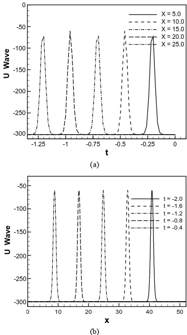
Figure 5. u wave (a) against t for different values of x (b) against x for different values of t.
x = 15.0, x = 20.0 and x = 25.0. Figure 5(b) describes u
wave increases against x for t = –2.0, t = –1.6, t =–1.2, t = –0.8 and t = 0.4. Interesting things are to be found in both cases, u wave gradually increases against t for dif-ferent values of x and against x for different values of t
before collision. As seen in Figure 6, u wave contour
against t and x. For the both cases we plot the phase
u for the Equation (14) with respect to time and displacement. As expected, we see that u wave contour
gradually increases like −324.161, −160, −55.8359 and so on over the domain [0, 40] × [–2, 0]. Next, contours of typical flow patterns are seen in Figure 7(a) which is
based on equation 15. The branch is composed of associ-ated over 0 ≤ t ≤ 2 and displacement 5 ≤ x ≤ 25. It is found that the flow oscillates irregularly that is multipe-riodic oscillation. We are also interested in trying our scheme for the wave solution of the K-dV equation. In
-324.161
-5 5 .8
35 9
-160
t
x
-2 -1.8 -1.6 -1.4 -1.2 -1 -0.8 -0.6 -0.4 -0.2 0
0 10 20 30 40 50
Figure 6. u wave contour against t and x.
t
0 0.25 0.5 0.75 1 1.25 1.5
X = 5.0 X = 10.0 X = 15.0 X = 20.0 X = 25.0
(a)
-50
-100
U W
ave
-150
-200
-250
(a)
x
0 10 20 30 40
t = 0.1 t = 0.5 t = 0.9 t = 1.3 t = 1.7
(b) 0
-50
-100
U W
ave
-150
-200
-250
(b)
[image:6.595.80.264.241.586.2]this figure we see that the behavior of the u wave is ex-actly what we expect in the analytical sense, the only thing that the change about the wave once in time for x =
5.0, x = 10.0, x = 15.0, x = 20.0 and x = 25.0 anywhere else about the wave stays the same. In Figure 7(b) we
see that wave solution follows that the exact solution fairly closely with respect to displacement over t = 0.1, t = 0.5, t = 0.9, t = 1.3 and t = 1.7. The general behavior of wave solution of K-dV equation remains same how-ever. Figure 8 describes u wave contour against t and x
over the domain [0, 40] [0, 2]. U wave contour is maximum on the top of the wave but diminishes from the top to both the sides of contour. Here, we see that at the top the value of the contour −100 and it gradually de-creases to the both sides like −260 to the left and −260 to the right. The plot of function (16) is shown in Figure 9(a) we have found u wave against t for different values
of x. In Figure 9(b) indicates that the u wave against x
for different values of t. Here we have seen that the u
wave against x for the different values of t like t = −2.0, t = −1.6, t = −1.2, t = −0.8 and t = −0.4, are exact to the previous one. For the both cases it shows that the waves are running against t and x respectively. Figure 10
de-scribes u wave contour against t and x over the domain [0, 25] [–2, 0]. Here u wave contour is maximum on the top of the wave but diminishes from the top to both the sides of contour. At the top the value of the contour is
−283.903 and it gradually decreases to the both sides like
−300 to the left and −300 to the right.
3.3. Case II
For the second case: 240
1 2
exp
2
G c c ,
1 2
2
exp
2
2
c c
G
Therefore,
2 1 2
c G
G c
-260
-260 -259.89
9
-100
t
x
0 0.2 0.4 0.6 0.8 1 1.2 1.4 1.6 1.8 2
[image:7.595.329.515.83.415.2]0 10 20 30 40
Figure 8. u wave contour against t and x.
t
-1.25 -1 -0.75 -0.5 -0.25 0
X = 5.0 X = 10.0 X = 15.0 X = 20.0 X = 25.0
(a)
0
-50
-100
U W
ave
-150
-200
-250
-300
(a)
x
0 10 20 30 40 50
t = -2.0 t = -1.6 t = -1.2 t = -0.8 t = -0.4
(b) -50
-100
U W
a
ve-150
-200
-250
-300
(b)
Figure 9. u wave (a) against t for different values of x (b) against x for different values of t.
-80
-283.903 -300
-299.99
-300
t
x
-1 -0.8 -0.6 -0.4 -0.2 0
[image:7.595.309.538.452.599.2]0 10 20
Figure 10. u wave contour against t and x.
Equations (F)-(J) and (10) implies respectively as fol-lows:
2 2
2
1 24
2
1
48 ;
2 8
c u
c
c c
x t
[image:7.595.61.307.456.720.2]
22 12 6
1 2 3
1
c u
c
c c x
24 12 2 1 2 12 2;1
16 , 0
c c
u
c c
x t
,
(18)
3 23
12 ;
1
c u
c
x
2
2
2
2 4 6
1 2
3 ,
1
c u
c
c c x
(19)
which is same as Equation
(20).
The numerical representation of two dimensional third order K-dV equation for this problem is obtained by the Fortran scheme compared with analytical solution to the following cases for 5.0, 6.25 and c = 12.0 such that 240 in the real sense. Numerical
solu-tion generates that the same behavior as solitary wave solutions for different cases. The solutions remain un-changed before and after their intersection. As seen in
Figures 11(a) and (a1) for the Equation (17), time
evaluation of u wave for different values of displacement like x = 5.0, x = 10.0, x = 15.0, x = 20.0 and x = 25.0. For a particular value of x = 10.0, u wave simply solitary. But the second case Figures 11(b) and (b1) for the same
equation, u-wave generates solitary for different values of t = −0.4, t = 0.0, t = 0.4, t = 0.8 and t = 1.2. Here
8 12 2 1 2 12 21
16 , 0
c c
u
c c
x t
;
20, 0 then,
12 ;
1
c
u x
c
(20)
t
0 0.1 0.2 0.3 0.4
X = 5.0 X = 10.0 X = 15.0 X = 20.0 X = 25.0
(a)
1000
0
-1000
U W
ave
-2000
-3000
-4000
-5000
t
0.1 0.12 0.14 0.16
X = 10.0
(a1)
1000
0
-1000
U
W
ave
-2000
-3000
-4000
-5000
(a) (a1)
x
0 25 50 75 100 125 150
t = -0.4 t = 0.0 t = 0.4 t = 0.8 t = 1.2
(b)
200
0
-200
U W
ave -400
-600
-800
-1200 -1000
150
x
-1 -0.5 0 0.5 1 1.5 2
t = 0.0
(b1)
200
0
-200
U W
ave-400
-600
-800
-1200 -1000
-1
(b) (b1)
Figure 11. u wave (a) against t for different va ues of x (b) against x for different values of t. l
negative sign of t indicates before the collision. For a particular value of t = 0.0 the u wave is solitary. In Fig- ure 12 shows that the contour is produced against t and x
simultaneously. In this equation we get the numerical representation of the solution of Equation (18) for
5.0
, 6.25 and c = 12.0 such that 240.
But for the values c = 10.0, c = 12.0, c = 15.0, c =17.0 we observe that u wave is solitary. For a particular value of c = 12.0, u wave generates solitary which is repre-sented in Figure 13(b). Next, contours of typical flow
pattern are seen in Figures 14(a) and (b) which is based
on Equation (19). The waves associate over the interval
−3 ≤x≤ 3. It is found that the flow oscillates regularly. We are also interested in trying our scheme for the wave solution of the K-dV equation. In this figure we have seen that the behavior of u wave is exactly that what we expect in the analytical sense, the only thing is that the
change about the wave once for the single value of c. For
Figure 14(a) the oscillation is no doubt solitary before
and after the collision for different values of c = 10.0, c
t
x
0 0.2 0.4 0.6
0 10 20 30 40
Figure 12. u wave contour against t and x.
x
-3 -2 -1 0 1 2 3
-3500
-3000
-2500
-2000
-1500
-1000
-500
0
C = 10.0 C = 12.0 C = 15.0 C = 17.0
U W
ave
x
-2 -1 0 1 2
-1500 -1000 -500 0
C = 12.0
U W
a
v
e
(a) (b)
Figure 13. u wave against x for different values of c.
x
-3 -2 -1 0 1 2 3
-3500
-3000
-2500
-2000
-1500
-1000
-500
0
C = 10.0
C = 12.0
C = 15.0
C = 17.0
U W
ave
U W
ave
x
-3 -2 -1 0 1 2 3
-3000 -2500 -2000 -1500 -1000 -500 0
C = 15.0
(a) (b)
U
W
ave
x
-3 -2 -1 0 1 2
-3500
-3000
-2500
-2000
-1500
-1000
-500
0
C = 0.4 C = 0.6 C = 1.5 C = 3.0
U W
ave
x
-3 -2 -1 0 1 2
-3500 -3000 -2500 -2000 -1500 -1000 -500 0
C = 0.6
[image:10.595.59.540.82.285.2](a) (b)
Figure 15. u wave against x for different values of c.
= 12.0, c = 15.0, c = 17.0. But in Figure 14(b) for a
par-ticular value of c = 15.0, the wave is very clear. The plot of Equation (20) is shown in Figures 15(a) and (b). We
have found wave against for different values of c. The waves against x for different values of c = 0.4, c = 0.6, c = 1.5, and c = 3.0 for λ = 5.0, μ= 6.25, and c = 12.0 such
that are exact that we have got in the
ana-lytical sense for the Equation (20). But in Figure 15(b)
represents a solitary wave against x for a particular value of c.
2 4
0
4. Conclusion
In this research numerical estimation of traveling wave solution for third order of two-dimensional K-dV equa-tion using a new auxiliary equaequa-tion method has been studied. The K-dV equation for the present problem comes from the third order two dimensional governing Equation (1.1) after some suitable transformation. It is found that there are nine exact traveling wave solutions (12)-(20) of 2-dimentional K-dV equation exist for real sense depends on different relevant physical parameters but the last one is exact the same as (20). Numerical re-sults of first ten cases for real sense obtained by using FORTRAN program have been shown graphically and discussed. We have also found that when employing the Fortran-Scheme for the numerical estimation of K-dV equation that are presented graphically for the first case
λ2 – 4μ> 0 and second case λ2 – 4μ> 0 Equations (12)-
(20). Remaining imaginary cases will be avenue of an- other research work in the future.
REFERENCES
[1] Yu. N. Zaiko, “Quasiperiodic Solutions of the Korteweg- de Vries Equation,” Technical Physics Letters, Vol. 28,
No. 3, 2002, pp. 235-236. doi:10.1134/1.1467286
[2] F. L. Qu and W. Q. Wang, “Alternating Segment Expli- cit—Implicit Scheme for Nonlinear Third-Order KdV Equation,” Applied Mathematics and Mechanics, Vol. 28, No. 7, 2007, pp. 973-980.
doi:10.1007/s10483-007-0714-y
[3] N. E. Zhukovskii, “Hydraulic Shock in water Pipelines,” Gostekhteorizdal, Moscow, 1949.
[4] A. C. Newell, “Solitons in Mathematics and Physics,” SIAM, Philadelphia, 1985.
[5] V. A. Rukavishnikov and O. P. Tkachenko, “The Korte- weg-de Vries Equation in a Cylindrical Pipe,” Computa- tional Mathematics and Mathematical Physics, Vol. 48, No. 1, 2008, pp. 139-146.
doi:10.1134/S0965542508010107
[6] N. Smaoui and R. H. Al-Jamal, “Boundary Control of the Generalized Korteweg-de Vries-Burgers Equation,” Non- linear Dynamics, Vol. 51, 2008, pp. 439-446.
[7] J. Pang, C.-Q. Bian and L. Chao, “A New Auxiliary Equa- tion Method for Finding Traveling Wave Solution to K- dV Equation,” Applied Mathematics and Mechanics (Eng- lish Edition), Vol. 31, No. 7, 2010, pp. 929-936.
[8] L. Debnath, “Linear Partial Differential Equations for Sci- entists and Engineers,” 4th Edition, Tyn Myint-U, 2007, pp. 573-580.
[9] R. L. Herman, “Solitary Waves,” American Scientist, Vol. 80, 1992, pp. 350-361.
[10] P. A. Clarkson and M. D. Kruskal, “New Similarity Re- ductions of the Boussinesq Equation,” Journal of Mathe- matical Physics, Vol. 30, No. 10, 1989, pp. 2201-2213.