http://www.scirp.org/journal/ica ISSN Online: 2153-0661
ISSN Print: 2153-0653
An Upper Limit for Iterative Learning Control
Initial Input Construction Using Singular Values
Naser Alajmi
1, Ali Alobaidly
2, Mubarak Alhajri
3, Salem Salamah
3, Muhammad Alsubaie
31Industrial Institute of Sabah Alsalem, PAAET, Kuwait, Kuwait 2Vocational Training Institute, PAAET, Kuwait, Kuwait
3Department of Electronics Engineering, College of Technological Studies, PAAET, Kuwait, Kuwait
Abstract
Selecting a proper initial input for Iterative Learning Control (ILC) algorithms has been shown to offer faster learning speed compared to the same theories if a system starts from blind. Iterative Learning Control is a control technique that uses previous successive projections to update the following execu-tion/trial input such that a reference is followed to a high precision. In ILC, convergence of the error is generally highly dependent on the initial choice of input applied to the plant, thus a good choice of initial start would make learning faster and as a consequence the error tends to zero faster as well. Here in this paper, an upper limit to the initial choice construction for the input signal for trial 1 is set such that the system would not tend to respond aggressively due to the uncertainty that lies in high frequencies. The provided limit is found in term of singular values and simulation results obtained illu-strate the theory behind.
Keywords
Iterative Learning Control, Initial Input Selection, Singular Values
1. Introduction
Iterative Learning Control (ILC) [1] is a control method that uses information obtained from previous executions/trials to update the next trial control input to enhance the performance of a repetitive system and accommodate periodic disturbances from trial-to-trial. ILC is adequate to repetitive systems where the reference trajectory has to be followed to a high level of accuracy infinite number of times.
Repetitive systems are those where the reference to follow, r t
( )
, has fixedHow to cite this paper: Alajmi, N., Alo-baidly, A., Alhajri, M., Salamah, S. and Alsubaie, M. (2017) An Upper Limit for Iterative Learning Control Initial Input Construction Using Singular Values. Intel-ligent Control and Automation, 8, 154-163.
http://dx.doi.org/10.4236/ica.2017.83012
Received: May 30, 2017 Accepted: July 18, 2017 Published: July 21, 2017
Copyright © 2017 by authors and Scientific Research Publishing Inc. This work is licensed under the Creative Commons Attribution International License (CC BY 4.0).
time duration, 0≤ ≤t T and has to be repeated large number of times which in turn tends to set the mathematical modelling expression outside the conventional control representation to a 2D system representation [2]. The idea of ILC came up as a consequence of human learning mechanism; for example, if a tennis player wants to learn how to hit a tennis ball with excellence, then he has to perform a large number of repetitions until he reaches perfection. This is ideally the learning principle of ILC where a system performs a successful operation in term of system stability within the operation time, measures the input u t
( )
, output (y t( )
) and calculates the error signal (e t( )
) and uses those information to update the next trial control input to enhance the performance in term of error norm trial-to-trial. The ILC control technique has a direct reflection on the industry and its applications; it can be seen in applications of pick and place such as robot arm, chemical batch processes, automated manufacturing plants and operations as such [3][4][5][6][7].The error signal (e tk
( )
) is the forcing part to update the upcoming control input. After each trial, a system has to be reset to its initial position to start the next one. The resetting time, known as the stoppage time, is the time required for a system to do all the needed computations to update the next trial control input signal to start the next trial. One approach of ILC is of the form1
k k k
u+ =u +Le , where uk is the trial k input; L is the learning gain and ek is
the trial k error signal. One good starting point for rich information about ILC Theory and applications is [8][9].
Repetitive control (RC) [10] is another control tool used to accommodate periodic disturbances through the use of previous trial informations. One major difference between ILC and RC is that in repetitive control, the initial conditions/states of a trial k+1 is the final states of trial k, while in ILC the
initial states are kept the same for all trials. This leads to a different application paradigm where RC is used to systems of continuous repetitive operations such as disc drives [11][12].
selection that combines each stored data with its weight to form the new input signal. Also [15] ¥ introduced another form of solution based on the presence of system model. This solutions directly depends on inverting the frequency component of the reference trajectory convoluted with the frequency component of the system model and sum as much as it is possible of the provided information to form the initial input signal. This theory does not give the limit at which a designer should stop in summing the frequency components. Every system representation is an approximate to the system behaviour, thus taking the inverse is critical in this issue due to system uncertainty and model mismatching. There are also several reported works regarding predicting trial information such as [17].
This paper sets an upper limit condition in constructing the initial input using singular values based on system presence. It is required in input construction that it would not generate a high effort at the beginning to assure safe operation. This development is highly required in most industrial applications such as in robot arms and chemical patch processes. In parallel it speeds up learning process compared to the same method when the initial input construction omitted. In order to do so, the upper limit condition guarantees safe construction for such input to fulfill the operation requirements.
The following section reintroduces the work presented in [15][16] that shows the relationship between the output required to obtain versus the initial input selection based on the presence of the system model. The new boundary condition that governs the initial input construction is introduced in Section 3. An examples of the use of the initial input on system learning process on a gantry robot arm is illustrated through simulation results is given in Section 4. Conclusion and future work are discussed in Section 5.
2. Initial Input Construction Based on System Knowledge:
Revisited
In term of understanding the initial input construction reported in [16], a brief introduction to Discrete Fourier Transform (DFT) is introduced as:
Let
( ) ( )
(
)
T0 1 1 N
u=u u u N− ∈ be an array of N elements, then (under the necessary assumption relating to existence) the DFT of this array, denoted by uˆ, is defined as
1 2π
0
ˆ e
N
j ni N
i n
n
u u
− − =
=
∑
(1) where ˆ N
u∈ and i=
{
0,1,,N−1}
. As mentioned earlier, ILC trajectoryreference has a fixed length of, T, and a sampling frequency must be chosen as
s
N f
T
= for N∈2 ,M M∈. The Inverse Discrete Fourier Transform (IDFT) can be driven to be
1 2π
0
1 ˆ e
N
j ni N
n i
i
u u
N
−
=
=
∑
then the convolution between g and u produces the output sequence
( )
(
) ( )
0
, 0,1, , 1
q
i
y q g q i u q q N
=
=
∑
− = −(3) The DFT of y can then be calculated using
ˆ ˆ ˆ
y=gu (4)
where is the component-wise multiplication.
Now, given a reference trajectory yd of length N and it is required to
construct an initial input vector * 0
u such that learning speed is improved when used with suitable ILC controller. In this paper an ILC law of the form
1
k k k
u+ =u +Le (5)
will be considered where L is chosen to be the adjoint of the process matrix G,
with
( ) ( )
(
)
T0 1 1
k k k k
u =u u u N− , and
( )
( )
( )
( )
(
)
(
)
T0 0 1 1 1 1
k d k d k d k
e =y −u y −u y N− −u N− . Let the associated LTI plant be given in state-space form of the following form
(
1)
( )
( )
x q+ =Ax q +Bu q
( )
( )
, 0,1, , 1y q =Cx q q= N−
(6) where the sample time has been set at unity for notational simplicity,
( )
nx ⋅ ∈ ,
( )
0 0x = , and the operators A, B and C are of appropriate dimensions. Then using the plant model yk=Guk [18], where
2 3
0 0 0
0 0
0
N N
D
CB D
G CAB CB D
CA − B CA −B D
= (7)
with
( ) ( )
(
)
T0 1 1
k k k k
y =y y y N− , is the lift form, then the error evolution equation can be driven easily to be
(
)
1
k k
e+ = I−GL e
(8) Taking the DFT of both sides of (5) now gives
1 ˆ
ˆk ˆk ˆk
u + =u +le (9)
and likewise for (8)
(
)
1 ˆ ˆ
ˆk ˆ ˆk
e+ = I−g l e
(10) where ˆ N
I∈ and has each entry equal to unity. Repeated application leads to
(
)
1 ˆ ˆ 0
ˆk ˆ k ˆ
e+ = I−gl e
(11) where the power operation is applied in component-wise fashion. Now consider the error progression starting from an arbitrary initial input, u0,
(
)
21 2 1 2
1 1, 0,
0 0
1 2 2 1 2 2
0, , 0,
0 0
ˆ
ˆ 1 ˆ ˆ
ˆ ˆ
ˆ ˆ ˆ ˆ ˆ ˆ
1 1
N N k
k k i i i i
i i
N k N k
i i i i i d i i i
i i
e e g l e
g l e g l y g u
This is minimized with respect to the initial input by setting uˆ0 equal to
, * 0,
ˆ
ˆ , 0,1, , 1
ˆ d i i
i
y
u i N
g
= = −
(13) This effectively generates a steady-state inverse (over the duration of the trial). The above derivation is found in [16] where more detailed description can be found there for cases that include system uncertainty for example. In (13), there is a lack in considering the maximum number of frequency components to include in constructing the initial input for trial 1. This was an open question and had been pointed as a possible area for further investigation. In the next section, and based on a submitted work by the author, a new condition is found that contains the number of frequency components to include in constructing the initial input based on the plant model presence. The new condition gives the upper limit of the initial input in term of singular values properties.
3. Setting an Upper limit to Constructing an Initial Input to
ILC
This section represents the novelty of this paper where a new condition is found that sets the maximum number of frequency components to include in constructing the initial input for trial 1 in any selected ILC method based on the presence of the plant model. This construction is as pointed out earlier includes system model presence. The key start was to consider the ILC design given in
[19], where part of the given design was discussed and load disturbances were added to form the new presented work in [20]. The major finding of that work was the load disturbance limitation such that the system will perform well and error will tend to low value based on the singular values as follows
( )
( )
1( )
1( )
1( )
0 0
0 0 0 0
k k k k
k i j h v
i j h v
d d Gu d Gu
σ σ − σ − −
= = = =
< Ψ − − − Ψ − −
∑
∑
∑
∑
(14)where d is the load disturbance, Ψ is the system output with the presence of load disturbances given by [20] and
( )
. and( )
. represent the maximum andminimum singular values respectively
(
)
( ) ( )
( )
,k t δ G q uk t dk t
Ψ + = + (15)
( )
( )
( )
, 0,1, , 1.k k k
y t = Ψ t +n t t= n−
(16) G is the process matrix and u0 is the initial input for the first trial. Here in this argument, two cases are to consider where the first is to assume that disturbances influence is still acting on the system while starting the operation; and this is a very small possibility in term of quality production. The second case is to consider system operation after the disturbances influence is vanished. Thus, in this case we can assume dk=dk−1=dk−2=d0. Now, we go through the following to find the upper limit to the initial input for the first trial
( )
1( )
0 0
0 0
0 0
k k
i h
i h
Gu Gu
σ σ −
= =
< Ψ − − − Ψ −
( )
( )
1
0 0
0 0
k k
h i
h i
Gu Gu
σ − σ
= =
Ψ − < Ψ −
∑
∑
(18)Breaking up the last equation leads to
(
)
(
)
( )
1( )
0 0
0 0
k k
i h
i h
Gu Gu
σ σ σ σ −
= =
− < Ψ − Ψ
∑
∑
(19)
(
0)
( )
0
k i i
Gu
σ σ
=
< Ψ
∑
(20)where σ
(
Gu0)
, and(
( )
)
1 0 kh h
σ −
= Ψ
∑
are assumed to be zero for simplicity. Thus, the result obtained in (20) says that for a linear repetitive system to start its operation with better performance, a designer can use the above inequality as a guide or reference when constructing the initial input such that the condition above is met. This condition says if a designer has the performance of first three trials in any previous operation, those information can be used to set the initial input according to (20).4. Simulation Results
[image:6.595.233.514.506.718.2]Simulation results presented in this section are obtained for a gantry robot Z-axis. The gantry robot shown in Figure 1 has been the benchmark for several ILC developed methods either in simulation or experimentally. The gantry robot represents a robot arm that is used in several industrial applications especially those of pick and place operations. The gantry performance accuracy, error convergence rate and robustness are important issues to a manufacturer, therefore its initial start represent an important issue for enhancing the performance and reducing the error convergence for the first trials. The gantry is constructed of three orthogonal axes where the Z-axis is the shortes axis fixed over the X and Y horizontal parts of the gantry and it consists of a ball-screw stage driven by a rotary brushless linear DC motor. The Z-axis of a 3rd order
representation and given as in [21]
( )
(
15.8869(
)(
850.3)
)
353.81 461.03 353.81 431.03
X
s G z
s s j s j
+ =
+ + + − (21)
For enhancing system performance, stability and disturbance rejection, the gantry system is fitted in a feedback loop with a PID controller whose parameters can be found in [15].
One common ILC method is the adjoint method addressed in; for example,
[22], where the equation that governs the new control input is of the form
1
T
k k k
u+ =u +βG e , where GT is the adjoint operator, and β is the step size. This algorithm had been proven to result a monotonic convergence along the trial domain [18].
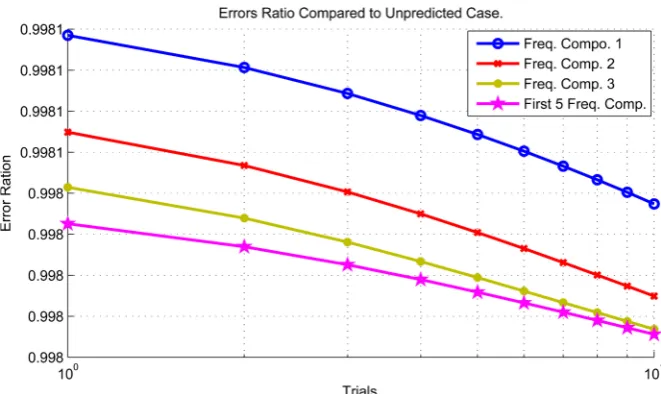
In this paper, the step size is chosen to be 0.5 and the system is operated for 10 trials; to show the advantage of using input prediction over the unpredicted case. The input is constructed using (13) for the first 5 frequency components and it showed an advantage of using an input with such construction method. In this example, the model given is treated as an exact model due to the fact that those results are obtained in simulation, but for the case of experimental implementation, it would be very sensitive in constructing the input and (20) should be considered since all models are an approximation to the exact behaviour.
Figure 2 shows reconstruction of the reference signal using the frequency
components 1, 2, and 3 individually and a reconstruction using the first 5 frequency components summed together. The more the frequency components used, the more accurate the reconstruction is. This idea had been projected over the initial input construction using (13) to form u0 for first trial operation.
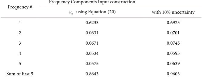
Applying (20) as an upper limit to the construction of u0 leads us to next table where the first column represents the frequency component while the second represents the result of applying (20). It can be seen that for the first 5 frequency component and the sum of the first 5 frequency components, the norm of u0 is still less than 1, thus there is no harm to use the sum of the first 5 frequency components to construct u0 according to (20).
Frequency # Frequency Components Input construction
0
u using Equation (20) with 10% uncertainty
1 0.6233 0.6925
2 0.0631 0.0701
3 0.0671 0.0745
4 0.0534 0.0593
5 0.0575 0.0639
[image:7.595.206.540.547.678.2]Sum of first 5 0.8643 0.9603
Figure 2. Reference construction from frequency components.
Figure 3. Error norms ratio plot for the predicted case over the unpredicted case.
error norm here is for an array of 1500 points representing the reference length; T Ts, where T is the length of the reference in seconds (3 s) and Ts is the sampling period which is 1/500 s.
Overall the initial input construction provides better error start which in turn speeds up learning process depending on the ILC method chosen and enhances the repetitive system performance. Notice the uncertainty effect where it clearly shows an increase in the control effort as the number of frequency components increases in constructing u0. Thus the condition given in (20) minimizes the effect of the uncertainty depending on limiting the first trial control effort by not exceeding the limit in (20).
5. Conclusions and Future Work
[image:8.595.208.539.278.475.2]a lack of setting an upper limit for the initial input construction reported in [19]
such that the system operation starts from the optimum choice of u0. Here the upper limit derived sets the number of frequency components to consider to construct the initial input according to design given there. The condition found is based on the principles of the singular values and remedies the lack of setting the upper limit. Simulation results show the advantage of using initial input over the case where the initial input construction is omitted.
In future, verifying the proposed work experimentally over the gantry is under consideration. Checking the validity of the proposed condition over different types of systems such as minimum-phase plants will be investigated experimentally in the future.
References
[1] Arimoto, S., Kawamura, S. and Miyazaki, F. (1984) Bettering Operation of Robots by Learning. Journal of Robotic Systems, 1, 123-140.
https://doi.org/10.1002/rob.4620010203
[2] Rogers, E., Galkowski, K. and Owens, D. (2007) Control System Theory and Appli-cations for Linear Repetitive Processes. Springer (Lecture Notes in Control and
In-formation Sciences),Berlin Heidelberg.
[3] Lee, J.H. and Lee, K.S. (2007) Iterative Learning Control Applied to Batch Processes: An Overview. Control Engineering Practice, 15, 1306-1318.
[4] Cho, W., Edgar, T.F. and Lee, J. (2008) Iterative Learning Dual-Mode Control of Exothermic Batch Reactors. Control Engineering Practice, 16, 1244-1249.
[5] Tayebi, A., Abdul, S., Zaremba, M.B. and Ye, Y. (2008) Robust Iterative Learning Control Design: Application to a Robot Manipulator. IEEE/ASME Transactions on Mechatronics, 13, 608-613.https://doi.org/10.1109/TMECH.2008.2004627
[6] Freeman, C.T. (2011) Constrained Point-to-Point Iterative Learning Control. IFAC Proceedings, 44, 3611-3616.
[7] Nygren, J., Pelckmans, K. and Carlsson, B. (2014) Approximate Adjoint-Based Iter-ative Learning Control. International Journal of Control, 87, 1028-1046.
https://doi.org/10.1080/00207179.2013.865144
[8] Bristow, D.A., Tharayil, M. and Alleyne, A.G. (2006) A Survey of Iterative Learning Control. IEEE Control Systems, 26, 96-114.
https://doi.org/10.1109/MCS.2006.1636313
[9] Ahn, H.-S., Chen, Y.Q. and Moore, K.L. (2007) Iterative Learning Control: Brief Survey and Categorization. IEEE Transactions on Systems, Man, and Cybernetics, Part C: Applications and Reviews, 37, 1099-1121.
https://doi.org/10.1109/TSMCC.2007.905759
[10] Hara, S., Omata, T. and Nakano, M. (1985) Synthesis of Repetitive Control Systems and Its Application. 24th IEEE Conference on Decision and Control, Lauderdale, Florida, 11-13 December 1985, 1384-1392.
[11] Moon, J.H., Lee, M.N. and Chung, M.J. (2002) Repetitive Control for the Track- Following Servo System of an Optical Disk Drive. IEEE Transactions on Control Systems Technology, 6, 663-670.https://doi.org/10.1109/87.709501
[12] Chen, Y.-Q., Moore, K.L., Yu, J. and Zhang, T. (2008) Iterative Learning Control and Repetitive Control in Hard Disk Drive Industry—A Tutorial. International Journal of Adaptive Control and Signal Processing, 22, 325-343.
[13] Arif, M., Ishihara, T. and Inooka, H. (2001) Incorporation of Experience in Iterative Learning Controllers Using Locally Weighted Learning. Automatica, 37, 881-888. [14] Arif, M., Ishihara, T. and Inooka, H. (2002) Experience-Based Iterative Learning
Controllers for Robotic Systems. Journal of Intelligent & Robotic Systems, 35, 381-
396.https://doi.org/10.1023/A:1022399105710
[15] Freeman, C.T., Alsubaie, M., Cai, Z., Rogers, E. and Lewin, P.L. (2011) Initial Input Selection for Iterative Learning Control. Journal of Dynamic Systems, Measure-ment, and Control, 133, Article ID: 054504.https://doi.org/10.1115/1.4003096
[16] Freeman, C.T., Alsubaie, M., Cai, Z., Rogers, E. and Lewin, P.L. (2011) Model and Experience-Based Initial Input Construction for Iterative Learning Control. Inter-national Journal of Adaptive Control and Signal Processing, 25, 430-447.
https://doi.org/10.1002/acs.1209
[17] Cho, B., Owens, D.H. and Freeman, C.T. (2016) Iterative Learning Control with Predictive Trial Information: Convergence, Robustness, and Experimental Verifica-tion. IEEE Transactions on Control Systems Technology, 24, 1101-1108.
https://doi.org/10.1109/TCST.2015.2476779
[18] Hatonen, J.J., Owens, D.H. and Ylinen, R. (2003) A New Optimality Based Repeti-tive Control Algorithms for Discrete-Time Systems. Proceedings of the European Control Conference (ECC03), Cambridge.
[19] Freeman, C.T., Alsubaie, M.A., Cai, Z., Rogers, E. and Lewin, P.L. (2013) A Com-mon Setting for the Design of Iterative Learning and Repetitive Controllers with Experimental Verification. International Journal of Adaptive Control and Signal Processing, 27, 230-249.https://doi.org/10.1002/acs.2299
[20] Alsubaie, M. and Rogers, E. (2017) Designed Iterative Learning Control via State Feedback in Past and Current Errors Schemes Robustness and Load Disturbances Conditions. The Journal of Systems and Control Engineering.
[21] Ratcliffe, J.D. (2005) An Iterative Learning Control Implemented on a Multi-Axis System. PhD Thesis, School of Electronics and Computer Science, University of Southampton, Southampton.
[22] Hatonen, J.J., Owens, D.H. and Moore, K.L. (2004) An Algebraic Approach to Itera-tive Learning Control. International Journal of Control, 77, 45-54.
https://doi.org/10.1080/00207170310001638614
Submit or recommend next manuscript to SCIRP and we will provide best service for you:
Accepting pre-submission inquiries through Email, Facebook, LinkedIn, Twitter, etc. A wide selection of journals (inclusive of 9 subjects, more than 200 journals)
Providing 24-hour high-quality service User-friendly online submission system Fair and swift peer-review system
Efficient typesetting and proofreading procedure
Display of the result of downloads and visits, as well as the number of cited articles Maximum dissemination of your research work
![Figure 1. Gantry robot as a test facility [21].](https://thumb-us.123doks.com/thumbv2/123dok_us/7738827.707405/6.595.233.514.506.718/figure-gantry-robot-test-facility.webp)