Logarithmic Sine and Cosine Transforms and Their
Applications to Boundary-Value Problems Connected with
Sectionally-Harmonic Functions
Mithat Idemen
Engineering Faculty, OKAN University, Istanbul, Turkey Email: [email protected]
Received September 30, 2012; revised January 8, 2013; accepted January 15, 2013
ABSTRACT
Let
r,
stand for the polar coordinates in R2, a0 be a given constant while u r
,
satisfies the Laplace equation u 0 in the wedge-shaped domain 0
, :r
0,a ,
j, j1
1
n
j
D r
or
. Here
, :
r a, , j, j 1
1
n j
D r
j
j1, 2, , n1
denote certain angles such that jj1. It isknown that if u r
, satisfies homogeneous boundary conditions on all boundary lines inaddition to non-homogeneous ones on the circular boundary
j
j1, 2, , n1
ra, then an explicit expression of u r
, in terms of eigen-functions can be found through the classical method of separation of variables. But when the boundary condition given on the circular boundary is homogeneous, it is not possible to define a discrete set of eigen-functions.In this paper one shows that if the homogeneous condition in question is of the Dirichlet (or Neumann) type, then thelogarithmic sine transform (or logarithmic cosine transform) defined by
ra
0
F sin logr d
a
s
f r
(or
0
fc r F cos log d
r a
) may be effective in solving the problem. The inverses of these transformations are
expressed through the same kernels on
0,a
or
a,
. Some properties of these transforms are also given in four theorems. An illustrative example, connected with the heat transfer in a two-part wedge domain, shows their effective-ness in getting exact solution. In the example in question the lateral boundaries are assumed to be non-conducting, which are expressed through Neumann type boundary conditions. The application of the method gives also the neces-sary condition for the solvability of the problem (the already known existence condition!). This kind of problems arise in various domain of applications such as electrostatics, magneto-statics, hydrostatics, heat transfer, mass transfer, acoustics, elasticity, etc.Keywords: Integral Transforms; Harmonic Functions; Wedge Problems; Boundary-Value Problems; Logarithmic Sine
Transform; Logarithmic Cosine Transform
1. Introduction
Boundary-value problems connected with sectionally- harmonic functions in wedge-shaped domains
0 1
, : 0, , ,
n
j j j
D r r a
1
and
1
1
, : , , ,
n
j j j
D r r a
,where
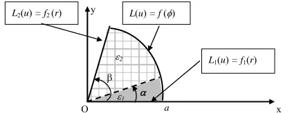
r, stand for the polar coordinates in R2 while a > 0is a given constant, are important from both purescientific and engineering points of view. Figure 1
epitomizes a simple caseof D0which corresponds to n = 2. The sub-regions determined by
0,
and
,
model the regions filled with different mate-rials having different constitutive parameters. The field function u r
, satisfies the basic equation
gradu ,
a x
O y
L2(u) = f2(r) L(u) = f ()
L1(u) = f1(r)
1
[image:2.595.67.278.86.168.2]2
Figure 1. A composite region D0 filled with two different
materials.
in the sense of distribution under the boundary conditions
1 1 , 2 2
L u f r L u f r
and
L u f
shown on the figure. Here F r
stands for the density of the exciting sources concentrated on the inter-face (if any) while L u
,L u1 and L u2
are given linear (differential) boundary operations. The boundary conditions in question may also involve certain terms representing the sources localized on the boundary (if any). As to the function
, it has constant values1 and 2 in the sub-regions in question. Thus on the in-terface between the sub-regions two transmission condi-tions of the following forms are satisfied:
, 0
, 0
0 u r u r , (1b)
2
2 u r, 0 1 u r, 0 r F r
. (1c)As is well-known, when F r
f r1
f2
r 0, one can define a set of orthogonal eigen-functions which permit us to obtain an explicit expression of u r
, in terms of these eigen-functions. The coefficients in the eigen-function series are determined by using the non- homogeneous boundary condition given on the boundaryr = a (i.e. throughf
) together with the regularitycondition to be stated at r = 0. When , at least
one of the functions
0f
, 1F r f r and f2
r must be different from zero in order to have a non trivial solution. In this case it is not possible to define a set of discrete eigen-functions. To overcome such kind of a difficulty, in the midst of the last century some methods, which are effective when the region consists of D0, were proposed. Among them we can mention, for example, the finite Sturm-Liouville transforms introduced by Eringen [1] and Churchill [2], and the finite Mellin transform introduced by Naylor [3,4] (see also [5]). The finite Sturm-Liouville transforms are not appropriate in the case considered here because they are based on the set of eigen-functions which can not be defined in the present case. As to the finite Mellin transforms, they are defined
as follows (see, for ex., [5, pp. 462-467]): 0
u
2 1
1 1
0
d ,
a s s s
a
M f r r f r r
r
(2a)
2 1
2 1
0
d .
a s s s
a
M f r r f r r
r
(2b)One can easily check that the first or the second trans-form is appropriate to reduce the Laplace equation writ-ten in the circular polar coordinates to an ordinary dif-ferential equation when Dirichlet or Neumann type con-ditions are prescribed, respectively, on the circular part r
= a of the boundary. The inverse transforms consist then
of the classical Mellin type integrals.
The aim of this note is to show that the transforms of the forms
0
sin log d
s
r
f r F
a
(3a) and
0
cos log d
c
r
f r F
a
(3b) are effective in getting explicit expressions to thesolu-tions of the problems connected with sectionally-har- monic functions defined in D0 and D mentioned above
when the boundary condition on the arc r = a is
homo-geneous and of the Dirichlet or Neumann type. The sim-plicity of these transforms is that their inverses are also given with the same kernel (see Section 2B below). To clarify the essential properties of the representations ((3a), (b)), in what follows we will consider, without loss of generality, the case where n = 1 (see Figures 2 and 3).
To the best of our knowledge a representation of the form (3b) was first considered by Smythe (see [6, pp. 71-72]) to find the electrostatic potential due to a line source located parallel to a dielectric wedge for which
0,
r . His discussion is based on moot physical
ar-guments and some particular restrictions. As we will show later on, a representation of the form (3b) is not suitable when r
0,
because only the data knownfor r
0,a or r
a,
is sufficient to uniquely2
a x
O y
D0
1
L2(u) = f2 (r) L(u) = 0
[image:2.595.314.527.594.710.2]L1(u) = f1(r)
a x
y
D
D
1
2 L(u) = 0
[image:3.595.64.279.85.185.2]L2(u) = f2(r) L1(u) = f1 (r)
Figure 3. A wedge-shaped region involving only the singular
etermine point r = .
d F
(i.e. the inverse transform).Further-more, when (3b) is used to express fc
r for all
0,
r , it gives fc
r fc
a r2 , which notac-om physics
is ceptable fr point of view.
2. Logarithmic Sine and Cosine Transforms
Let a > 0 be a given constant while F
L1
0,
isa given function. Then consider the functions fs
r and fc
r defined through the convergent integral ing p (3a) and (3b). There log stands for theprin-cipal branch of the logarithm function. We will refer
s
s tak-lace in
f r and fc
r to as the logarithmic sine transformgarithmi sine transform of F
and lo c co , respectively.
In what follows we will also denote them by the symbols
S F and C F
. Some interesting and important pro- of thes nsforms are stated in the theorems given below.perties e tra
A) Limit Values for r
0, r
a and r
As we will see later on (see Section 2B), the expression of the function fs
r (or fc
r ) known only in the interval
0,a or
is ent to determine the function
,a suffici
F uniquely. The functions fs
r and
c
f r m iece-wise continuous in thes vals.
eans that the limit values of the integrals taking place in (3a) and (3b) as r tends to the end point
0 or or
r ra r may be different from the values
irectly r0 orraorr in
those integrals. From applicati the limiting values that are important. Therefore these limit
values must be discussed carefully. The two theorems that follow concern this point (for their proof see Appendix).
Theorem-1. If
ay be
by repl
p
acing d
e inter That m
obtained
on point of view it is
1 0,
F L , then from (3a) one
ge
(4a)
Theorem-2. a) If then from (3b)
on ts
0
lim 0,
lim 0 0 ,
lim 0 .
s s
r a
s s
r
s s
r
f r f a
f r f
f r f
1
0,
F L ,
e gets
0
lim 0 0 ,
lim 0 .
c c
r
c c
r
f r f
f r f
(4b)
b) If one has also
F
L1
0,
, then
lim c c 0.
ra f r f a (4c)
B) Inverse Transforms when
It is an interesting fact that fs
r (or fc
r ) isknown for all r
0,a or for all a, , th the functionr
en
F can be determine tely. The theorems th llow concern this inversion problem (for their proof see Appendix). Notice that when
d comple at fo
f r is piece-wise continuous, in what follows f r
means
0
0
2.f r f r
Theorem-3. a) Let fs
r L1
0,l
a be piece-wise
continuous in the interva 0,a
and fs
a 0. Then (3a) yields
0
2 d
sin log , 0, .
π a
s
F f
a
(5a)b) If fc
r L1
0,a is piece-wise continuous in theinterval
0,a , then (3b) yields
0
2 d
cos log , 0, .
π a
c
F f
a
(5b)Theorem-4. a) Let fs
r L a1
,
be piece-wisecontinuous for r
a,
and fs
a 0. Then (3a)yields
2
sin log d ,
0,
.π s a
F f
a
(6a)b) If fc
r L a1
,
is piece-wise continuous for
,
r a , then from (3b) one gets
2
cos logd ,
0,
.π c a
F f
a
(6b)The proof of these theorems (except Theorem 1) can easily be achieved by using the already known ones through simple transformations (See for example [5] or [7]). For the sake of fluency of the paper, we prefer to postpone the proofs to the Appendix. In what follows we will denote the inverse transforms given by (5a) and (6a) by 1
s
S f r . Similarly, the inverse transforms given
by ( will be denoted by 1
C f r .
5b) and (6b) c
3. Applications to Boundary-Value Problems
W lso
Connected with Sectionally-Harmonic
Functions
hen one has a 2
1
0,F L
and (3b) one gets
2
sin logrr rf r F
0
d
s
a
(7a)and
2
0
cos log d
c
r
r rf r F
a
, (7b)which show that
1
2
1s s
r rf r S f
S (8a) and
1 (8b)
Now consider a function
1 2
c c
C r rf r C f .
,u r which is harmonic in
1
or
and satisfies a homogeneous boundary condition of the
0 , : 0, , ,
j
j j
D r r a
1
, : , , ,
j
j j
D r r a
Dirichlet or Neumann type on the circular part of the
boundary, namely:
2
2 0
u u
r r
r r
(9)
and
, 0,
j, j 1
u a (10a) or
, 0,
j, j1
u a
r
. (10b)
Application of the operator 1 or
S C1 to (9) yields
2
2ˆ , d ,
u u
2 ˆ 0, (11) d
((8a), (b)) being taken into account. Here uˆ ,
orm of stands for the logarithmic sine or cosine transf
,u r . From (11) one gets
, A sinh
1ˆ
cosh , , ,
j j
j j j
u
B
j
(12)where Aj
0
, A sinh
cosh sin log d
j j
j j
u r
r B
a
(13a)
or
0
, sinh
cosh cos log d
j j
j j
u r A
r B
a
. (13b)
(13a) is valid for the condition (10a) while (13b) is valid
Application
esentations ((13a), for the case of (10b).
4. An Illustrative
To show the effectiveness of the repr
(b)), in what follows we will give an illustrative example which concerns the heat conduction in a two-part com-posite region shown in Figure 4. A point source of
amount Q exists at the point (b, 0) while the circular part
of the boundary is coated by an insulating material. The physical properties of the lateral boundaries (i.e. the
boundary conditions on and ) will be defined later on. Thus the field function (temperature)
,u r satisfies the following field equation under the
given boundary conditions:
,
, , ,
r b b r a
gradu , Q div r
(14)
,
,
1
,
u
r u r f r r
n r
, a
(15a)
,
,
2
,
u
r u r f r r a
n r
,
(15b)
,
, 0,
u
a u a
n r ,
(15c)
,
1 asu r O r r . (15d)
y
x
O
2
1
a b
u/n = f2(r)
r
Q
n
n
x
O
2
a
u/n = f1(r)
u/n = 0
Q
n
1
and Bj
ugh th
are the integration constants to be d ed thro e boundary and transmission conditions while
etermin
j
and j are two constants which
can be chosen appropriately to facilitate the computation. They may also be dependent on . Thus, in the sector
j, j1
[image:4.595.318.541.418.709.2]Here
has constant values 1 and 2 in the indi-cated sub-re ions.let us write g
Remark that the problem posed by (14)-(15d) has a
solution if th
1
2
, , , 0 ,
, , 0, . u r
u r
u r
(17) e following necessary condition is satisfied
by the boundary conditions :
ud Since the field Equation (14) is equivalent to the equa-tionsD
s Q
n
(16a) or, more explicitly,
0
(16b)
This is obtained by first integrating (14) o
, 0, ,
u r r D
(18a)
, 0
, 0
0,
,u r u r r a
(18b)
f r
1
1
d 2 2
da a
r f r r Q
n D
and
and
2 , 0 1 , 0 ,
, ,
u r u r bQ r b
r a
(18c) then applying the Green’s theorem. In what follo we
will assume that (16b) is satisfied (it will be used later on!).
In accordance with the definitions of
ws
and Q, one can write
1
0
, cosh cosh cos logr d ,
u r A B
a
(19a
)
2
0
, cosh cosh cos logr d .
u r C D
a
(19bThe coefficients
)
1 2
1
1 2
1 2
sinh cosh cos log
2 ,
π sinh
D
b a Q
, ,A B C and D
are determined through 5a), (15b b) and (18c) as follows:
the conditions (1 ), (18
(20c)
Here we put
1
A
2
, sinh
, sinh C
(20a)
1 1
2 2
2 cos log d ,
π
2
cos log d .
π
a
a
r
f r r
a
r
f r r
a
2 1
2
1 2
1 2
sinh cosh
cos log
2 ,
π sinh
B
b a Q
(20b)
(21)
If we first insert (20a)-(20c) into ((19a), (19b)) and then use the Euler formula to write the cos function through exponential functions, then we get
1 2 2 1
1
1 2
1 2
1
, cosh cosh e d
sinh sinh cosh
2
cosh
cos log e d
π sinh
i i
u r
b Q
a
(22a)
and
2 1 1 2
2
1 2
1 2
1
, cosh cosh
sinh sinh cosh
2
cosh
cos log e d
π sinh
i i
u r
b Q
a
e d
where is defined with Remark. It is worthwhile to notice here that the
con-vergence of the inverse transform integrals in (22a) and (22b) requires the relation (23). That m
tion stated by (23) is in fact a condition for the existence of the solution. One can easily check that this is nothing but (16b) (or (16a)). This shows that the application of th
logr 0. a
(22c)
Now it is important to observe that the point 0, to be a which is located on the i
double pole of the inte
ntegration line, seems
grands in (22a) and (22b). But because of the relation (16b) these poles are removable.
Indeed, the removability of these dition
poles requires the
con-
1 1 2 2
2
0 0 0,
πQ
(23)
which is equivalent to (16b), (21) being taken into ac-count. Since the expressions taking place in the brackets in (22a) and (22b) are even functions of , (23) guaran-tees the removability of the singularity at = 0. Thus, on
the basis of Jordan’s lemma, the integral
can be computed through the residues at the poles located s in ((22a), (b)) in the upper
J0
or lower
J0
half-planes. The residue series coming from the poles which occur at the zeros of sinh() and cosh() are connected with the geometry of the wedge in question and, hence, con-sist of the eigen-functions series. But the terms coming from the poles of 1
and 2
(if any!) areindependent o metry of th and have no connection with the eigen-functions.
f the geo e wedge
eans that the
rela-e transformation in qurela-estion dorela-es not only prela-ermit us to obtain an explicit expression of the solution but rather shows also the necessary conditions for the existence of a solution.
4.1. A Particular Case. Point Sinks Located on the Lateral Boundaries
Assume more particularly that
, 2
,1
f r M rc f r M rc (24a) where c
a and M stand for two given constantsuch that (Cf. (23) or (16b))
s
1 2
M Q 0. (24b) In this case the lateral boundaries consist ofmaterials and carry sinks at the points
insulating
c,
and
c,
. By straightforward computations one gets
1 2
2 cos
π log ,
M c
a (24c) which reduces (22a) to
2
log
1
log log
1 2
e +e d
d . sinh
i rc a
i rc a i r b
2
log
i r c
1
2
cosh ,
2π sinh
cosh 2π
Q u r
Q
e +e
Since in the present case one always has
(25)
2
1, 2
1, 0, 0,rb a rc a
hich yields w
exp
0sinh exp
as
cosh exp
in 0 or 0
cosh exp exp
0
sinh exp
as in 0 or 0,
by the Jordan’s lemma, the first parts of these integrals can be computed by considering the residues of the poles taking place in the upper half-plane . But, de-pending on the relative positions of r one can get
0 h
J
and c,
r c 1 or
r c <1. Therefore the s rt of the first integral involves the contribution e polesex-isting in half-plane or (similar situation is also valid for p e second integral). Thus, we have t er t ng four cases sep :
Case 1: case 2: Case 3:
econd pa s of th
the Jh0 h
the second o consid
b c r case 4:
0
J
art of th he followi
.
c a
arately
, rb c r
, a,
b r
By straightforward computations we get the following results:
1
1
1 2
,
π
1
, cos
π
π
cos
n
n
r b c
n Q
u r n
n
Q
n
2
a
2 1
1 2
π n n a
π π
π π
1
n
c
n n
br r
b
cr r
(26a)
1 2
1 1 2
2 1
1 2 ,
π π
1 π
, cos
π
π π
1cos π π
n n
n
r b c
n n
cr r
Q
u r n
n a c
n n
br r
Q
n
n a b
(26b)
1 2
1
1 2
2 1
1 2
π π
1 π
, cos
π
π π
1cos π π
n
n
n
b r c
n n
cr r
Q
u r n
n a c
n n
br r
Q
n
n a b
(26c)
1 2
1
1 2
2 1
1 2
π
1 π
, cos
π
π π
1 π
cos
π
n
n
n
c r b
n n
cr r
Q
u r n
n a c
n n
br r
Q
n
n a b
π
(26d)
By comparing (22b) with (22a) one observes that
2 , 1 ,
u r u r esting to compare ( the case of 1 2
, where . It is also inter-26a)-(26d
0, result pertinent toa
) with the
. T two-part wedge prob ous wedge problem
hus on that the present lem is equi o the
with eter
e concludes valent t constitutive param
1 2 2
.
5.
transfo
us Dirichlet or Neumann boundary conditions on the
circular part of the boundary of wedge shaped domains.
pli-REFERENCES
[1] A. C. Eringen, “The Finit
Quarterly Journal of Mathematics
pp. 120-129.doi:10.1093/qmath/5.1.120
Conclusions and Concluding Remarks
From the analysis made above one concludes that the logarithmic rmations defined by (3a) and (3b) may be appropriate in getting explicit expressions of sec- tionally-harmonic functions which satisfy the homoge-neoThis kind of problems arise in various domain of ap cations such as electrostatics, magneto-statics, hydrosta- tics, heat transfer, mass transfer, acoustics, elasticity, etc.
e Sturm-Liouville Transform,” , Vol. 5, No. 1, 1954, [2] R. V. Churchill, “Generalized Finite Fourier Cosine
Transforms,” Michigan Mathematical Journal, Vol. 3, No. 1, 1955, pp. 85-94.doi:10.1307/mmj/1031710540
[3] D. Naylor, “On a Mellin Type Integral Transform,”
Journal of Mathematics and Mechanics, Vol. 12, No. 2, 1963, pp. 265-274.
[4] D. Naylor, “On an Integral Transform of the Mellin Type,” Journal of Engineering Mathematics, Vol. 14, No. 2, 1980, pp. 93-99.doi:10.1007/BF00037619
[5] I. N. Sneddon, “The Use of Integral Transforms,” McGraw- Hill Co., New York, 1972.
[6] W. R. Smythe, “Static and Dynamic Electricity,” McGraw- Hill Co., New York, 1950.
Appendix. Proof of Theorems
1. A Proof for Theorem-1
0s
f a is quite obvious. To find the limit of fs
r for ra,consider first the case when r
a,
and assume that an arbitrarily fixed (small) 0 is given. Since
1
0,
F L , we can find an R0 such that
d .4
F
R
(27a) Thus, from (3a) one gets
0s
0
sin log F
a
in log sin log d
R
r r
F
a a
sin l
R
r
ogr d a
s s
f r f r
which yie
lds
0
2 sin .
2
R
F
r
log 1 d
s s
f r f r
(27b)
Now, by taking into account the
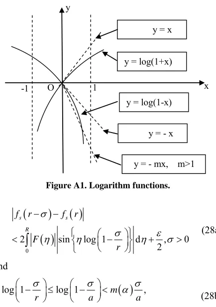
ure A1).
inequalities (see
Fig-log 1 log 1 ,r a a
r a
(27c)
and
sinx x x, 0, we can choose so small that
0
2 F s
0 0
in log 1 d
2 d 2 d .
R R
r
R
F F
a a
2
(27d)
From (27b) and (27d) we conclude that for every
0
, however it is small, we can find 0 such that
,s s
f r f r ra
which permits us to write
0
,s s .
f r f r ra
For this gives the first equati in (4a). To prove the same equality for the case of
ra on
0,r a ,
and repeat we choose an arbitrary number
the arguments made above by re
0,a placing by
. nchanged All the lines except (27b) and (while the latter become now as follows: 27c) remain u
x 1
y = log(1- x) y = log(1+x) y
y = x
O -1
y = - x
[image:8.595.315.532.79.387.2]y = - mx, m>1
Figure A1. Logarithm functions.
02 sin log 1 d ,
2 0
F
r
s s
R
f r f r
(28a)and
log 1 log 1 ,
.
m
r a
a r
a
(28b)
Here m
1 pend onstands for a suitable number which does not de (For detail see Figure A1). Thus, by
choosing sufficiently small, we guarantee
0
2 d ,
2
R
m F
a
(28c)which yields
s s
f r f r
and
0
,s s .
f r f r ra
For r =a the latter reduces to the first equality in (4a)
(28d)
when r
0, .asee the lim
To fs
r0
it of as r0, consider an
arbi-trarily given (small) and choose such that the second part in A 0
0sin log d
sin log d
F
a
r F
a
A s
A
r
f r
(29a)
meets the following inequality:
sin
F log d d .
2
A A
r
F a
After having fixed A, let us make . By virtue of
the well-known Riemann-Lebesgue [5, p. 30], the part in (29a) tends to zero wh
0
r
lemma en
first log
one ha
r a .
Therefore, for sufficiently small r s also
0sin log d .
A
r F
2
a
(29c)
nc
From (29a)-(29c) one co ludes that for sufficiently small r one has fs
r for every 0. Thisproves the second equality in (4a).
(29a)-(29c) are also valid for r, which shows the
last equality in (4a)
2. A Proof for Theorem-2
The equalities given in (4b) can be shown by repeating Theorem-1. As to the equality given in (4c), owing to the assumption
the reasoning made in proving
1
0,
F L
and
0
1 sin log d ,
c
r
f r F
r a
(30) it is reduced to the first equality in (4a).
3. Proofs of Theorem-3 and 4
. 34])
If
Proof of these theorems are based on the following well- known lemma (see [5, p .
Lemma (Fourier’s integral theorem). f t
is piece-wise continuous and absolutely integrable in
,
, then for all x
,
one has
1
0 0 .
2 0
d cos
π
1 d
f t
x t t
f x f x
(31)
) and make the substitutions
Let us insert (5a) into the right-hand side of (3a
loga 0, ,loga 0,
r
(32a)
which yield
d
e , e , d
a r a
(32b)
and
0 0
2 e sin d sin d .
π fs a
0
sin logr d
F
a
3a) (3
Now let us define the odd function
e 1
f a L ,
0s
f a ):
as follows (notice that
e
fs
ae
, 0f a
e , 0.s
f a
(33b) Then (33a) can also be written as
0
0
sin log d
1
e sin d sin d
π
r F
a
f a
or
(33c)
0
d e cos
π f a
0
sin log d
1 d .
r F
a
(33d)
Since the function f a
ea, from
meets the requirements the last expression one mentioned in the lemm
gets
0
0 sin log d
1 0 0 , 0, .
2 s s
r F
a
0 1
e e
2 f a f a
f r f r r a
(34)
This proves (5a).
To prove (5b), one starts from (3b) and repeats (32a)- the only exception that (33b) is replaced now ven function
Proof of theorem-4 is quite similar to that of
Theo-re rence is
(34) with by the e
e
e
, 0 e , 0.c
c
f a
f a
f a
m-3. The only diffe that and defined in (32a) are replaced now by
log a 0,
and
log r a 0,