The Monetary Model of Exchange Rate
in Nigeria: an Autoregressive Distributed
Lag (ARDL) Approach
Evans, Olaniyi
Department Of Economics, University Of Lagos, Nigeria
December 2013
Online at
https://mpra.ub.uni-muenchen.de/52457/
Nigeria: an Autoregressive Distributed Lag
(ARDL) Approach
Olaniyi Evans
Abstract
This study examines the monetary model of exchange rate in Nigeria, using an
Autoregressive Distributed Lag (ARDL) approach over the period 1998Q1 to 2012Q2. The
estimation results show that there is long run relationship among variables of the monetary
model of exchange rate for Nigeria. That is, the estimated coefficients of the money supply,
income and interest rate differentials support the monetary exchange rate model. As well,
the stability test of CUSUM shows that there exists a significant and stable monetary model
of exchange rate determination for Nigeria. Therefore, this study recommends that market
participants in the foreign exchange market may monitor and forecast future exchange rate
1. Introduction
The Bretton Woods system collapsed, to be replaced by the floating exchange rate system
in 1973. Since then, volatility of exchange rates has been intractable. The character of
exchange rate and its sway on the functioning of macroeconomies has continued to spawn
interest among economists and policymakers. Mordi (2006) argued that the exchange rate
movements have effects on inflation, price incentives, fiscal viability, competitiveness of
exports, efficiency in resource allocation, international confidence and balance of
payments equilibrium. To a large extent, misalignment in real exchange rate could twist
productive activities, thwart exports and engender instability in an economy.
An exchange rate is the current market price for which one currency can be exchanged for
another. For instance, if the Naira exchange rate for the United States Dollar stands at 155,
this means that ₦155 can be exchanged for $1. For the reason that exchange rates’ role in a country's competiveness level is substantial, exchange rates are among the most analysed
and forecasted indicators in the world. Exchange rate is governed by the level of supply
and demand on the international markets. Yet, changes in exchange rates are not amenable
to prediction because the market is outsized and volatile. In fact, according to
tradingeconomics.com (2013), the currency markets are the most liquid in the world with
a daily turnover of close to $2 trillion.
The long run model of exchange rate determination has been the subject of intense interest
for many researchers. The monetary approach has been used to understand exchange rate
movements. Several models explaining exchange rate behaviour have been developed.
Over the past four decades, the monetary approach to understanding exchange rates has
become the prevailing model of exchange rate determination (Diamandis and Kouretas,
1996). Within the monetary approach to exchange rate determination, there are two
variants: the flexible- price monetary model (Frankel 1976; Bilson, 1978) and the
sticky-price monetary model (Dornbush, 1976). According to the monetary exchange rate model,
a relationship exists between the nominal exchange rate and monetary fundamentals. That
purchasing power parity (PPP). Therefore, this model provides a long-run benchmark for
the nominal exchange rate between two currencies. As well, it establishes a standard for
determining whether a currency is “overvalued” or “undervalued” (Rapach and Wohar,
2002).
Prior studies on long run relationship between exchange rate and the monetary variables
have their weaknesses. Their standard approach to testing the monetary exchange rate
model has been through the cointegration techniques of Johansen-Juselius (1990) and
Johansen (1991). Examples include Jimoh (2004), Nwafor (2006), Long and Samareth
(2008) and Liew et al. (2009). By using Johansen-Juselius cointegration technique and the
assumption that all variables are I(1), the studies are flawed. It is common knowledge that
in order to conduct Johansen-Juselius cointegration test, all variables must be integrated of
the same order. Yet, the studies failed to consider this factor in their analysis and went
ahead to use variables of different orders. In order to subdue this error, this study uses
ARDL approach to cointegration. The advantage of ARDL approach is that it tests the
cointegrating relationship without any necessity for same order of integration for all
variables.
The purpose of this paper is to fill the gap in the literature by re-examinining the validity
of the monetary exchange rate model in Nigeria using an advanced econometric technique,
that is to say, Autoregressive Distributed Lag (ARDL) approach. Evidence of the monetary
model in Nigeria is little with the few available studies testing for Johansen-Juselius
cointegration with variables of different orders. This study solves that problem by using
ARDL approach which is not susceptible to such problems.
The remainder of the paper is structured as follows: section 2 provides a brief overview of
the Nigerian exchange rate regime. Section 3 outlines a review of the empirical literature
on the monetary exchange rate model. Section 4 presents the theoretical framework for the
monetary exchange rate model. Section 5 describes the methodology and data used in the
2 Overview of Nigerian Exchange Rate Regime
In the beginning, Nigeria practiced a fixed exchange rate policy, where the Naira was
pegged against the British pound and afterwards the American dollar. However, there was
the termination of the Bretton Woods international system of fixed exchange rates in the
early 1970s. Since then the international monetary system advance with copious and
conspicuous developments. Many countries forsook pegged exchange rates and instead
either (1) practise a monetary policy based on flexible exchange rate or (2) connect
monetary policy to other countries through a monetary union or dollarization. Consequent
upon these developments, Nigeria adopted a flexible exchange rate policy, allowing the
Naira to float and its value relative to the American dollar controlled by market forces of
demand and supply.
Various policies have been employed in Nigeria to ensure exchange rate stability. These
included among others: Second-Tier Foreign Exchange Market (SFEM), Autonomous
Foreign Exchange Market (AFEM), Inter-bank Foreign Exchange Market (IFEM), the
Enlarged Foreign Exchange Market (FEM), and the Dutch Auction System (DAS).
Generally, the hopelessness and flop of each policy to help and achieve stability in the
exchange rate invariably leads to the espousal of another.
To the chagrin of all endeavors to maintain exchange rate stability by avoiding its
fluctuations and misalignment, the Naira continues to depreciate against the American
dollar. For example, the Naira appreciated against the American dollar in the 1970s. It
depreciated throughout the 1980s. The exchange rate became relatively stable in the
mid-1990s, then it depreciated further till 2004. Thereafter, it appreciated from 2005, till 2007.
Summarily, from 1960 until 2013, the exchange rate averaged 119.0900 reaching an
all-time high of 164.8000 in December of 2011 and a record low of 0.5300 in October of 1980.
The incessant depreciation have been attributed to the decline in the nation's foreign
exchange reserves. The activities of speculators and banks are also blamable. The
voracious quest for abnormal profits has compelled some banks to engage in
(CBN) and sell to parallel market operators at prices other than the official prices. These
malpractices engender exchange rate fluctuations and misalignment. The exchange rate is
approximately N150 against the American dollar.
3 Literature Review
The monetary approach remains one of the several important tools employed to explain the
variation in exchange rates. In early 1980s, it appeared without doubt no empirical support
for this approach was established. Today, with better-quality statistical tools along with a
more exact specification of the model, the long-term validity of the monetary approach to
exchange rate determination has been established.
Dara Long and Sovannroeun Samreth (2008) examine the validity of short-run and
long-run monetary models of exchange rate for the Philippines, using Autoregressive
Distributed Lag (ARDL) approach. They find robust short-run and long-run relationships
between variables in the monetary exchange rate model. However, the Purchasing Power
Parity (PPP) condition fails and all the monetary restrictions are rejected. Therefore, they
conclude that the estimation of the monetary model of exchange rate, in which monetary
restrictions are assumed to be satisfied beforehand, might suffer from a number of
deficiency. That is, it is not proper to estimate the exchange rate model before the monetary
restrictions are confirmed.
Hwang (2001), using Johansen's multivariate cointegration, find up to three cointegrating
vectors between the exchange rate and macroeconomic fundamentals for the U.S.
dollar/Canadian dollar. That is, there is a long-run relationship between the exchange rate
and economic fundamentals. Based on error correction models, he finds that two monetary
models outperform the random walk model at the three-, six-, and 12-month forecasting
horizons. Therefore, he concludes that monetary exchange rate models are still useful in
Miyakoshi (2000), using Johansen-Juselius cointegration technique, examines the
flexible-price monetary model in Korea. He finds the Korean Won exchange rates to be cointegrated
with money supplies, incomes and interest with the US dollar, German mark and Japanese
yen as numeraires.
Shylajan, Sereejesh and Suresh (2011), using the Johansen- Juselius cointegration
technique, examines the link between the Indian rupee-US dollar exchange rates and the
macroeconomic fundamentals using the flexible-price monetary model. The outcomes
reveal the existence of long-run relationship between exchange rate and the
macroeconomic variables, validating the flexible-price monetary model. Nonetheless, no
short-run causal relationship was found, using the vector error-correction model.
Conversely, a strand of the literature finds little evidence in support of the monetary
exchange rate model. For example, Cusham (2000) finds a cointegrating relationship for
the monetary model using Canadian–US dollar exchange rate in which the estimated
cointegrating coefficients are inconsistent with the monetary model predictions. Thus he
concludes that the monetary model is not validated.
Nieh and Wand (2005), using both Johansen’s (1988, 1990, 1994) maximum likelihood
cointegration test and the ARDL Bound test by Pesaran, Shin, and Smith (2001) for
Taiwan, examines Dornbusch’s (1976) sticky-price monetary model to exchange rate determination. They find ambiguous results for the long-run equilibrium relationship
between the NTD/USD exchange rate and macro fundamentals. With the aid of ARDL
Bound test, they conclude that there is no long-run equilibrium relationship between
exchange rates and macro fundamentals.
For Nigeria, Nwafor (2006), using the Johansen’s multivariate cointegration technique,
examines the link between the naira-dollar exchange rates. He finds at least one
cointegrating vector for Nigeria, validating the existence of a long-run monetary model of
exchange rate. Alao et al. (2011), using Johansen cointegration framework as well,
outcomes reveal one cointegrating vector for Nigeria. They conclude that the variability of
the nominal naira-dollar exchange rate is consistent with flexible price model.
Adawo and Effiong (2013), using the Johansen (1991) and Johansen and Juselius (1990)
cointegration technique, examines the long-run validity of the monetary exchange rate
model in Nigeria for the flexible exchange rate regime. They find a unique long-run
relationship between the nominal exchange rate and money supply, output and interest rate
differentials. The estimated cointegrating coefficients are consistent with the monetary
model and statistically significant exception of the output differential.
To study the dynamic relationship between exchange rate and macroeconomic variables,
most studies have focused on the existence of a long-run relationship within the monetary
model framework using the conventional Johansen’s cointegration technique. Instead, the
purpose of this paper is to re-examine the exchange rate determination model using ARDL
(autoregressive distributed lag) Bound test by Pesaran, Shin, and Smith (2001) to
investigate the long-run and short-run impacts of monetary model to exchange rates during
1986:01–2003:04. In other words, we examine the long-run equilibrium relationship
between NGN/USD exchange rate and macro fundamentals of Nigeria and the US using
the ARDL approach. No other study has used this approach for Nigeria.
4 Theoretical Framework
Research studies on exchange rates stem from the equilibrium theory of supply and demand
(Nieh and Wand, 2005).
At equilibrium, the money supply is equal to money demand.
Md = Ms (1)
According to the Cambridge equation,
Ms = kPY (2)
To keep the exchange rate stable, the nominal exchange rate, E, is defined as domestic
currency value of a unit of foreign currency,
Therefore,
E =Ms k* Y*/Ms*kY (4)
Where Ms* and Y* are foreign money supply and real income.
Taking the log of (4),
e = (ms - ms*) – (y - y*) – (log k – log k*) (5)
e, ms, ms*, y, and y* are the logarithms of E, Ms, Ms*, Y and Y* respectively.
Now, the cost of holding money is expressed in terms of interest rate so that the demand
for real balances is:
ms– p = a + by – ci (6)
a, b, and c are constant parameters, and i is the nominal interest rate.
And for the foreign country,
ms* – p* = a + by* – ci* (7)
Taking the log of (3),
e = p – p* (8)
Putting (6) and (7) in (8),
e = (ms– ms*) – b(y – y*) + c(i – i*) (9)
According to (9), monetary theory proposes that exchange rates are a monetary
phenomenon influenced by money supply, income level, and interest rates.
Three models of the monetary approach to exchange rate came up in the 1970s. The
flexible-price monetary model, the sticky-price monetary model and the real-interest
differential model.
In the flexible-price monetary model (Frenkel, 1976), prices are flexible; they adjust
immediately in the money market. Domestic and foreign capital are perfect substitutes. The
Fisher equation (i = r + π) holds in both countries. r is the real interest rate. π is the expected
inflation rate.
Substitute for π for i and π* for i* in Equation (9),
e = (ms– ms*) – b(y –y*) + c(π –π*) (10)
Assuming different coefficients of demand for money in the two countries,
ms– p = ɧ1 + ɧ2y –ɧ3i (11)
Therefore, the monetary model of exchange rate in the unrestricted form is,
et = ɸ0 + ɸ1mst + ɸ2mst* + ɸ3yt + ɸ4yt* + ɸ5it + ɸ6it* + ξt (13)
In the monetary model of exchange rate, ɸ1 = 1,ɸ2 = -1, ɸ3 < 0, ɸ4 > 0, ɸ5 > 0 and ɸ6 < 0.
5. Model Specification and Methodology
The flexible-price monetary model of exchange rate in (13) can be expressed as
unrestricted error correction ARDL model,
Δet = ϰ0 + ∑ϰ1iΔet-I +∑ϰ2iΔmt-i + ∑ϰ3iΔmt-i* + ∑ϰ4iΔyt-i + ∑ϰ5iΔyt-i* + ∑ϰ6iΔit –I + ∑ϰ7iΔit-i* + ϒ1et-1 + ϒ2mt-1 + ϒ3mt-1* + ϒ4yt-1 + ϒ5yt-1* + ϒ6it -1+ ϒ7it-1* + Зt (14)
Where
∆ denotes the first difference operator,
ϰ0 is the drift component,
Зt is the white noise residuals.
The left-hand side is the exchange rate. The second until seventh expressions on the
right-hand side represent the short-run dynamics of the model. The remaining expressions with
the summation sign correspond to the long-run relationship.
To investigate the presence of long-run relationships among the variables, bound testing
procedure of Pesaran, et al. (2001) is used. After Pesaran et al. (2001), the ARDL bounds
testing approach has become the state-of-the-art technique for finding the long-run and
short-run relationships among time series variables. It is called the bounds testing approach
because it involves testing whether the calculated F statistics are within or outside two
bounds: the lower bound for I(0) and the upper bound for I(1).
The ARDL is chosen for this study because it can be applied for a small sample size as it
happens in this study. It can estimate the short and long-run dynamic relationships
simultaneously. ARDL precludes the need for testing the order of integration amongst the
variables and of pre-testing for unit roots, because the ARDL approach is valid regardless
if the underlying regressors are I(0) or I(1). With the ARDL, there is possibility that
The ARDL bound test is based on the Wald-test (F-statistic). The F-test is essentially a test
of the hypothesis of no cointegration among the variables against the existence of
cointegration among the variables, denoted as:
H0: ϒ1=ϒ2=ϒ3 =ϒ4 = ϒ5 = ϒ6 =ϒ7 = 0 i.e., there is no cointegration among the variables.
H1: ϒ1≠ϒ2≠ ϒ3 ≠ ϒ4 ≠ ϒ5 ≠ ϒ6 ≠ϒ7 ≠ 0 i.e., there is cointegration among the variables.
Two critical values are given by Pesaran et al. (2001) for the cointegration test. The lower
critical bound assumes all the variables are I(0) signifying that there is no cointegration
among the variables. The upper bound assumes that all the variables are I(1) signifying that
there is cointegration among the variables. When the computed F-statistic is greater than
the upper bound critical value, then H0 is rejected (the variables are cointegrated). If the
F-statistic is below the lower bound critical value, H0 is accepted (the variables are not
cointegrated). If the F-statistics is between the lower and upper bounds, then the results are
indeterminate.
The data are obtained from different sources, including International Financial Statistics
and CIA World Factbook.
.
6. Empirical Analysis of the Monetary Model
The main plus of this approach lies on the fact that ARDL methodology obviates the need
to classify variables into I(1) or I(0). Compared to standard cointegration, there is no need
for unit root pre-testing. The ARDL cointegration test assumes that only one long run
relationship exists between the dependent variable and the independent variables (Pesaran,
Shin and Smith, 2001).
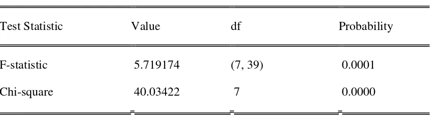
In the first step, F-statistics for judging whether there is a long run relationship among
Table 1 Wald Test
Test Statistic Value df Probability
F-statistic 5.719174 (7, 39) 0.0001
Chi-square 40.03422 7 0.0000
The results of table 1 show that F-statistic is significant. The F-statistics of the model is
bigger than the critical value of the case that all variables are I(1) both in 10% and 5%.
This result supports the evidence of long run cointegrating relationship. It shows that the
null hypothesis of no long run relationship can be strongly rejected. Therefore, it is evident
that there is long run relationship among variables in the model.
From the Wald test, the calculated F-statistic 5.719174 is higher than the upper bound
critical value 4.088 at the 5 percent level. Thus, the null hypothesis of no cointegration is
rejected, implying long run cointegration relationships amongst the variables. The
estimated coefficients of the long run relationship show that exchange rate is significantly
explained by the variables included in the analysis. The adjusted R-squared shows that 95.3
percent of the variation in exchange rate is explained by the variables. The F-statistic also
indicates that the model is significant. As well, the Durbin Watson statistic shows evidence
of no serial correlation.
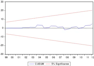
Now we use the tests of CUSUM and CUSUMQ to test the stability of the model. Figure
1 provides the graph of CUSUM test. It is categorically evident that the plot of CUSUM is
Fig 1 Plot of Cumulative Sum of Recursive Residuals (CUSUM)
This gives credence to the fact that there exists long run stability of the monetary model of
exchange rate in Nigeria.
7. Conclusion
This study has examined the validity of the monetary exchange rate model in Nigeria using
an Autoregressive Distributed Lag (ARDL) approach over the period 1998Q1 to 2012Q2.
The estimation results show that there is long run relationship among variables of the
monetary model of exchange rate for Nigeria. When the stability of the estimated model is
tested with CUSUM, it shows that there exists a significant and stable monetary model of
exchange rate determination for Nigeria.
Therefore, the estimated coefficients of the money supply, income and interest rate
differentials support the monetary exchange rate model. That is, the fluctuations in the
Naira/Dollar exchange rate depend and respond to the monetary fundamentals in the -30
-20 -10 0 10 20 30
99 00 01 02 03 04 05 06 07 08 09 10 11 12
[image:13.612.90.453.120.375.2]monetary exchange rate model. Therefore, this study recommends that market participants
in the foreign exchange market may monitor and forecast future exchange rate movements
REFERENCES
Bilson, J. F. O. (1978) “Rational expectations and the exchange rate” in The Economics of
Exchange Rates by J. A. Frankel and H. G. Johnson, Eds., Adison-Wesley Press: MA., 75
– 96
C. Nieh and Y. Wand (2005) ARDL Approach to the Exchange Rate Overshooting in
Taiwan. Review of Quantitative Finance and Accounting, 25: 55–71
Cusham, D. O. (2000) “The failure of the monetary exchange rate model for the Canadian –U.S. dollar” Canadian Journal of Economics, 33(3), 591 – 603.
Dara Long and Sovannroeun Samreth (2008) The Monetary Model of Exchange Rate: Evidence from the Philippines Using ARDL Approach Online at http://mpra.ub.uni-muenchen.de/9822/
Diamandis, P. F. and G. P. Kouretas. 1996. “The Monetary Approach to the Exchange Rate: Long-Run Relationships, Coefficient Restrictions and Temporal Stability of the
Greek Drachma.” Applied Financial Economics, 6: 351-362.
Dornbush, R. (1976) “Expectations and exchange rate dynamics” Journal of Political Economy, 84, 1161-1176.
Frankel, J. A. 1979. “On the Mark: A Theory of Floating Exchange Rates Based on Real
Interest Differentials. American Economic Review, 69: 601-622.
Frenkel, J. A. 1976. “A Monetary Approach to the Exchange Rate: Doctrinal Aspects and
Empirical Evidence.” The Scandinavian Journal of Economics, 78: 200-224.
http://www.tradingeconomics.com/nigeria/currency
J. Hwang (2001) Dynamic Forecasting of Monetary Exchange Rate Models: Evidence
from Cointegration. Ouachita Baptist University—U.S.A. IAER: FEBRUARY 2001,
VOL. 7, NO. 1
Johansen, S. (1991) “Estimation and hypothesis testing of cointegration vectors in Gaussian vector autoregressive models” Econometrica, 59, 1551-1580.
Johansen, S. and K. Juselius (1990) “Maximum likelihood estimation and inference on
cointegration –with applications to the demand for money” Oxford Bulletin of Economics
Long, D. and S. Samreth (2008) “The monetary model of exchange rate: evidence from the
Philippines using ARDL approach” Economics Bulletin 6, 1-13.
Miyakoshi, T., “The Monetary Approach to the Exchange Rate: Empirical Observations from Korea.” Applied Economics Letters 7(12), 791–794 (2000).
Monetary exchange rate model as a long-run phenomenon: evidence from Nigeria Monday A. Adawo and Ekpeno L. Effiong Department of Economics, University of Uyo, Nigeria 5. February 2013 Online at http://mpra.ub.uni-muenchen.de/46407/ MPRA Paper No. 46407
Mordi, N. O. (2006), "Challenges of Exchange Rate Volatility in Economic Management in Nigeria", In The Dynamics of Exchange Rate in Nigeria, Central Bank of Nigeria Bullion, Vol. 30, No. 3, pp. 17-25.
Nwafor, F. C. (2006) “The naira-dollar exchange rate determination: a monetary
perspective” International Research Journal of Finance and Economics 5, 130 – 135.
Nwafor, F. C. (2006) “The naira-dollar exchange rate determination: a monetary
perspective” International Research Journal of Finance and Economics 5, 130 – 135.
Rapach, D. E. and Wohar, M. E. (2002) “Testing the monetary model of exchange rate
determination: new evidence from a century of data” Journal of International Economics
58, 359–385.