Minkowski geometry and space time manifold in relativity

Munich Personal RePEc Archive

Minkowski geometry and space-time

manifold in relativity

Mohajan, Haradhan

Journal of Environmental Treatment Techniques

18 October 2013

Online at

https://mpra.ub.uni-muenchen.de/51627/

1

Minkowski Geometry and Space-Time Manifold in Relativity

Haradhan Kumar Mohajan Premier University, Chittagong, Bangladesh.

Email: haradhan_km@yahoo.com

Abstract

Space-time manifold plays an important role to express the concepts of Relativity properly. Causality and space-time topology make easier the geometrical explanation of Minkowski time manifold. The Minkowski metric is the simplest empty space-time manifold in General Relativity, and is in fact the space-space-time of the Special Relativity. Hence it is the entrance of the General Relativity and Relativistic Cosmology. No material particle can travel faster than light. So that null space is the boundary of the space-time manifold. Einstein equation plays an important role in Relativity. Some related definitions and related discussions are given before explaining the Minkowski geometry. In this paper an attempt has been taken to elucidate the Minkowski geometry in some details with easier mathematical calculations and diagrams where necessary.

Keywords: Causal structure, Geodesics, Ideal points, Minkowski metric, Space-time manifold.

1 Introduction

A manifold is essentially a space which is locally similar to Euclidean space in that it can be covered by coordinate patches but which need not be Euclidean globally. Minkowski space-time manifold plays an important role in both Special and General Relativity. To explain Minkowski geometry we need proper knowledge in differential manifold and causal properties of space-time. A brief discussion of manifold and causality has been given before discussing the Minkowski metric.

We cannot imagine relativistic problems without Einstein equations. Einstein equation in the presence of matter is given by [1];

µν µν

µν π T

c G R g

R 8 ₄

2 1

− =

− .

Minkowski metric is on the basis of empty space solution of Einstein equation. It is a flat space-time manifold M =

4

ℜ and is given by;

2 2 2 2 2

dz dy dx dt

ds =− + + + .

We have discussed its geometrical properties in section–5.

2 Manifold in Differential Geometry

Any point p contained in a set S can be surrounded by an open sphere or ball

x

−

p

<

r

, all of whose points lie entirely in S, where r>0; usually it is denoted by;

( )

p

r

{

x

d

( )

p

x

r

}

S

,

=

:

,

<

.

Let p be a point in a topological space (defined later in section 2.2) M. A subset N of M is a neighborhood of p iff

N is a superset of an open set O containing p, i.e.,

N

O

p

∈

⊂

.

A function f : A→B is a subset of A× B, such that i) if

A

x∈ , there is a set y∈B such that (x, y) ∈f ii) such an element y is unique , that is , if x∈A, y, z∈B such that

( )

x

,

y

∈

f

,

( )

x

,

z

∈

f

then y = z . If f :A→B is a function, then the image off,f

( )

A, is the subset of B

defined as follows: f

( )

A =

{

f

( )

x /x∈A

}

, that is, f

( )

A

consists of elements of B of the form

f

( )

x

, where x is some element of A. Here f is a map from A to B. A function f: A→B is one-one if each element of B is the image of some element of A. The function f is onto if for all x, y∈A,

( ) ( )

x

f

y

f

=

implies x = y. The function is one-one and onto if it is both one-one and onto.

Let _Rn _{be the set of n-tuples}

(

n

)

x

x1,..., of real numbers. A set of points M is defined to be a manifold if each point of M has an open neighborhood which is continuous one-one map onto an open set of _Rn

for some n.

A manifold is essentially a space which is locally similar to Euclidean space in that it can be covered by coordinate patches but which need not be Euclidean globally. Map

O O→ ′

:

φ

where n

R

O⊂ and m

R

O′⊂ is said to be a class Cr

(

r≥0

)

_{if the following conditions are satisfied. If} we choose a point p of coordinates

(

_{x x}n

)

,...,

1 _{on O and its}

image φ

( )

p of coordinates

(

x

′

1

,...,

x

′

n

)

on O′ then by

r

C

map we mean that the function

φ

is r-times differential and continuous. If a map is Crfor all r≥0 then we denote it by C∞; also by 0

C _{map we mean that the map is}

continuous. An n-dimensional,

C

r, real differentiable manifold M is defined as follows: Manifold M has a

r

C altas

{

U

_α

,

φ

_α

}

where U_α are subsets of M and

φ

_α are one-one maps of the corresponding U_α to open sets in _Rn

such that;

1. _Uα cover M i.e., M

α αU

2

2. If U_α∩U_β ≠

φ

then the map

(

α β

)

α

(

α β

)

β

β

α

φ

φ

φ

φ

o

−1

:

U

∩

U

→

U

∩

U

is a

C

r map of an open subset of

R

n to an open subset of n

R .

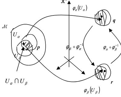
Condition (2) is very important for overlapping of two local coordinate neighborhoods (figure–1). Now suppose U_α

and U_β overlap and there is a point p in U_α∩U_β. Now

choose a point q in

φ

_α

( )

U_α and a point r in

φ

_β

( )

U_β .

ℜn

_φα

( )

U_α

•

q

M

Uα

•

p

φ

βo

φ

α−1 φαoφβ−1

U_β

•

U

_α

∩

U

_β r

[image:3.595.75.275.247.407.2]

φβ

( )

Uβ

Figure 1:The smooth maps

φ

_α

o

φ

_β−1 on the n

-dimensional Euclidean space ℜn_.

Now −1

( )

r

=

p

β

φ

,

φ

_α

( )

p

=

(

φ

_α

o

φ

_β−1

)

( )

r

=

q

. Let coordinates of q be

(

x

1

,...,

x

n

)

and those of r be

(

n

)

y

y

1

,...,

. At this stage we obtain a coordinate transformation;

(

n

)

x

x

y

y

1

=

1 1

,...,

(

n

)

x

x

y

y

2

=

2 1

,...,

… … …

(

n

)

n n

x

x

y

y

=

1

,...,

.

The open sets U_α,

U

_β and maps −1

β

α

φ

φ

o

and −1

α

β

φ

φ

o

are all n-dimensional, so that

C

r manifold M _{is r-times}

differentiable and continuous i.e., M is a differentiable manifold.

2.1 Space-time Manifold

General Relativity models the physical universe as a four-dimensional C∞ Hausdorff differentiable space-time manifold M _{with a Lorentzian metric g of signature}

(

−

,

+

,

+

,

+

)

which is topologically connected, paracompact and space-time orientable. These properties are suitable when we consider for local physics. As soon as we investigate global features then we face various pathological difficulties such as, the violation of time orientation, possible non-Hausdorff or non-papacompactness, disconnected components of space-time etc. Such pathologies are to be ruled out by means of reasonable topological assumptions only. However, we like to ensure that the space-time is causally well-behaved. We will consider the space-time Manifold (M_{,g) which has no}

boundary. By the word “boundary’ we mean the ‘edge’ of the universe which is not detected by any astronomical observations. It is common to have manifolds without boundary; for example, for two-spheres S2 in ℜ3 _{no point} in S2 is a boundary point in the induced topology on the same implied by the natural topology on _ℜ3_{. All the} neighborhoods of any 2

S

p∈ will be contained within S2

in this induced topology. We shall assume M to be connected i.e., one cannot have M=_X∪_Y, where X and Y

are two open sets such that X∩Y≠ϕ. This is because disconnected components of the universe cannot interact by means of any signal and the observations are confined to the connected component wherein the observer is situated. It is not known if M is simply connected or multiply connected. M _{assumed to be Hausdorff, which ensures the}

uniqueness of limits of convergent sequences and incorporates our intuitive notion of distinct space-time events.

2.2 Topology and Tangent Space

A topological space in a manifold is defined as follows: Let S be a non-empty set. A class T of subsets of S is a topology on S if T satisfies the following three axioms [3]:

i. S and

φ

belong to T,

ii. the union of any number of open sets in T belongs to T, and

iii. the intersection of any two sets in T belongs to T. The members of T are open sets and the space (S, T) is called topological space.

A k

C -curve in M is a map from an interval of _ℜ in to

M (figure–2). A vector

( )

( )t0

t

λ

∂

∂

which is tangent to a

1

C -curve

λ

( )

t at a point

( )

0 t

λ is an operator from the space of all smooth functions on M into ℜ and is denoted by [2];

( )

_{( )}

( )

( )

( )

[

]

[ ]

( )

s t f s t f Lim t

f f

t t _t s

λ

λ

λ λ

− + =

     

∂ ∂ = ∂

∂

→0

0 0

3

•

λ

( )

b

λ

( )

t

•

•

λ

( )

a

λ

•

•

•

a t b

[image:4.595.130.223.113.262.2]

Figure 2: A curve in a differential manifold.

If

{ }

i

x are local coordinates in a neighborhood of

( )

t0

p=λ then we get;

( ) _{( )}

0 0

.

t i i

t

x

f

dt

dx

t

f

λ

λ

∂

∂

=













∂

∂

_.

Thus every tangent vector at p∈M can be expressed as a linear combination of the coordinates derivates,

( ) ( )

n _p

p x

x ∂∂

∂ ∂ _,...,

1 . Thus the vectors

( )

i

x

∂

∂ span the

vector space

p

T . Then the vector space structure is defined by

(

α

X+

β

Y

)

f =

α

( ) ( )

Xf +

β

Yf . The vector space T_pis also called the tangent space at the point p.

A metric is defined as;

ν µ

µν

dx

dx

g

ds

2

=

; µ,ν =1,2,3,4 (1)

where _gµν is an indefinite metric in the sense that the

magnitude of non-zero vector could be either positive, negative or zero. Then any vector X∈T_p is called timelike, null or spacelike if;

(

X,X

)

<0, g

(

X,X

)

=0, g

(

X,X

)

>0

g . (2)

An indefinite metric divides the vectors in _Tp into three disjoint classes, namely the timelike, null or spacelike vectors. The null vectors form a cone in the tangent space

p

T which separates the timelike vectors from spaelike vectors (figure–3). When the manifold has dimension four then it is called a space-time manifold and signature of the metric of the manifold is +2. The tangent vector for a particle travelling with a constant velocity less than that of light through a point p in such a space-time is represented by a timelike vector at p.

3 Causality and Space-time Topology

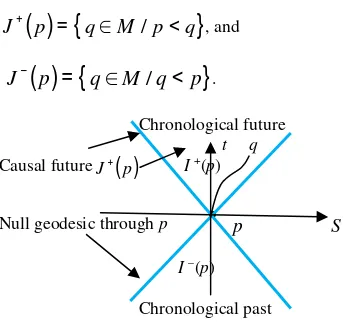
Given an event p in M, the lines at 450 to the time axis through that event give null geodesics in M. Such null geodesics form the boundary of the chronological future or past I±

( )

p of an event p which contains all possible timelike material particle trajectories through p including timelike geodesics [1, 2]. The causal future J+

( )

p is the

closure of I+

( )

p , which includes all the events in M, which are either timelike or null related to p by means of future directed non-spacelike curves from p. An event p

chronologically precedes another event q, denoted by p <<

q, if there is a smooth future directed timelike curve from p

to q. If such a curve is non-spacelike then p causally precedes q i.e., p < q. The chronological future I+

( )

p and past I −

( )

p of a point p are defined as (figure–3).

( ) {

p

q

M

p

q

}

I

+

=

∈

/

<<

, and

( ) {

p q M q p

}

I− = ∈ / << .

The causal future (past) of p can be defined as;

( ) {

p

q

M

p

q

}

J

+

=

∈

/

<

, and

( ) {

p

q

M

q

p

}

J

−

=

∈

/

<

.

Chronological future t q

Causal futureJ+

( )

p I +(p)

Null geodesic through p

•

_{p S}

I –(p)

Chronological past

Figure 3: Causality and chronology in MMMM....

Also p<<q and q<r or

p

<

q

and

q

<<

r

implies

r

p

<<

. Hence,

( )

p

J

( )

p

I

+

=

+ and

I

&

+

( )

p

=

J

&

+

( )

p

.

4 Einstein Field Equations Riemann curvature tensor;

β µν α βσ β µσ α βν α

σ µν α

ν µσ α

µνσ

=

Γ

;

−

Γ

;

+

Γ

Γ

−

Γ

Γ

R

(3)

[image:4.595.316.488.353.514.2]

4

    

  

∂ ∂

∂ − ∂ ∂

∂ − ∂ ∂

∂ + ∂ ∂

∂

= _σ ρν_µ

ρ ν µσ ρ

σ µν µ

ν ρσ ρµνσ

x x

g x x

g x x

g x x

g R

2 2

2 2

2

1 ₊

(

λ

)

ρν α µω λ ρσ α µν

αλ

Γ

Γ

−

Γ

Γ

g

. (4)

Ricci tensor is defined as;

.

λµσν λσ

µν g R

R =

(5)

Further contraction of (5) gives Ricci scalar;

λσ λσ

R g

Rˆ= (6)

The energy momentum tensor Tµνis defined as;

ν µ

µν _{ρ u u}

T = 0 (7)

where ρ₀ is the proper density of matter, and if there is no

pressure, and

dt dx X u

µ µ

µ_{= = is a tangent vector. A perfect}

fluid is characterized by pressurep=p

( )

xµ , then;

(

)

µ ν µν

µν _{ρ p u u pg}

T = + + (8)

where ρ is the scalar density of matter. The principle of local conservation of energy and momentum states that;

0

; =

µν ν

T .

Einstein’s field equations can be written as [4];

µν µν

µν π T

c G R g

R 8 ₄

2

1 ₌₋

− (9)

where _G=_6.673×₁₀−11 _{is the gravitational constant and}

8

10 =

c m/s is the velocity of light.

5 Minkowski Space-time

The Minkowski space-time (M, g) is the simplest empty space-time in general relativity, and is in fact the space-time of the special relativity. Mathematically it is the manifold

M = _ℜ4

and so that metric (1) for Lorentzian case becomes [4];

2 2 2 2 2

dz

dy

dx

dt

ds

=

−

+

+

+

(10)

where

−

∞

<

t

,

x

,

y

,

z

<

∞

. Here coordinate t is timelike and other coordinates x, y, z are spacelike. This is a flat space-time manifold with all the components of the

Riemann tensor

R

_νλσµ

=

0

. So the simplest empty space-time solution to Einstein equation is;

0 8 =

= _µν

µν

π

T

G (11)

which underlies of the physics of special theory of relativity. Under Lorentz transformation the Minkowski metric preserves both time and space orientations. The vector

t

∂

∂ provides a time orientation for this model.

In spherical polar coordinates

(

t

,

r

,

θ

,

φ

)

, where t = t,

φ

θ

sin sin

r

x= , y=rsin

θ

cos

φ

and z=rcos

θ

then (10) takes the

2 2 2 2

2

=

−

+

+

Ω

d

r

dr

dt

ds

(12)

with

0

<

r

<

∞

,

0

<

θ

<

π

,

0

<

φ

<

2

π

and

2 2 2 2

sin

θ

φ

θ

d

d

d

Ω

=

+

. Here coordinate t is timelike and other coordinates

r

,

θ

,

φ

are spacelike. There are two apparently singularities for r = 0 and

sin

θ

=

0

; however this is because the coordinates used are not admissible coordinates at these points, i.e., we used spherical polar coordinates and the frames are now non-inertial. That is why we have restriction of

r

,

θ

,

φ

as above and we need two such coordinate neighborhoods to cover all of the Minkowski space-time, then (12) will be regular. We assumed that all the components of the Riemann curvature tensor vanish for the Minkowski space-time which is a flat space-time. In

(

t,x,y,z

)

coordinates this is very clear that all the metric components are constant, i.e., diagonal

(

−

,

+

,

+

,

+

)

, so all the connection coefficients, Γ’s, will vanish. But in spherical polar coordinates

(

t,r,θ,φ

)

, the connection coefficients , Γ’s, will not vanish, for example,

r

=

Γ

1

22 ; however all the Riemann curvature components

will still vanishes,

R

_νλσµ

=

0

i.e., the manifold is still gravitation free, i.e., flat space-time [1, 2].

The Lorentz transformations on the Minkowski space-time are defined as the set of those metric preserving isometries (a metric is isometries if

g

_µν

( )

x

=

g

_µν

( )

x

from the transformation of one inertial i

x to i

x) which are linear and homogeneous transformations. Physically these represent the change of reference frame from one inertial observer to another inertial observer. Hence the Lorentz transformations are defined by the coordinate change;

µ ν µ ν µ

µ

_x

_L

_x

_x

x

→

′

=

=

L

(13)

From the above and the fact that these are metric preserving isometries, it follows that detL_νµ=±1, so the matrix is non-singular. If _det µ₌₁

ν

L and further 0 1

0≥

5

µ

µ µ

µ _{Lx LLx L x}

x′′ = ₁ ′ = ₁ = ₂ , (14)

where LL₁≠L₁L, i.e., Lorentz transformation forms a non-Abelion group.

The set of all the Lorentz transformations form a group where the identity map is given by

δ

_νµ

=

I

₄ and the inverse is defined by inverse matrix _L−1_{. The Poincare}

group is defined by;

T L + = + =

′ µ ν

ν ν µ ν

µ _{Lx T x}

x , (15)

where T denotes transformation matrix.

So, Lorentz group is a sub-group of Poincare group of transformations which are general inhomogeneous mapping that leave the general mapping consists of a Lorentz transformation together with an arbitrary transformation in space and time. This is ten parameter group, consisting of six Lorentz parameters (six rotations in space-time are;

(

, 1,2,3,4

)

; =

∂ ∂ − ∂

∂

= i j

x x e x x e

M j j j _i i

i

ij

, where

e

i

=

1

for i = 1,2,3 and ei =−1 for i = 4) and four translation

parameters 

  

 

= ∂

∂

= ;i 1,2,3,4

x L

i i

, and represents

physically a mapping of one inertial frame onto another in general position in the space and time. These isometries form the ten parameter Lie group of isometries of flat space-time known as inhomogeneous Lorentz group which is Poincare group.

In a coordinate system in which the metric takes (10), the geodesics γ have the form,

x

µ

( )

v

=

b

µ

v

+

c

µ, where bµ

and cµ are constants. Here

c

µ

≠

0

gives a new choice of the initial point γ

( )

0 and bµ≠0 implies the

renormalization of the vector X. Thus the exponential map

M T

ep: p→ is given by;

( )

e

X

X

x

( )

p

x

µ _p

=

µ

+

µ , (16)

where Xµ are the components of X with respect to the

coordinate basis       ∂

∂

µ x

of T_p. Since

e

_p is one-one and

onto, it is a diffeomorphism between

p

T and M. Thus any

two points of M can be joined by a unique geodesic curve. As

e

_p is defined everywhere on

p

T for all T, (M, g) is geodesically complete. So, there is no singularity in Minkowski geometry. The geodesics of Minkowski space-time are the straight lines of the underlying Euclidean geometry.

An arbitrary event p in the Minkowski space-time is uniquely determined either by its chronological future

( )

p

I+ or past I −

( )

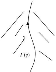
p .

If a future directed non-spacelike curve γ has a future end point p, then I−

( )

γ =I−

( )

p (_I−

( )

γ _{is the union of all I}−

( )

_q with q being a point on the curve γ). On the other hand, if

γ is future inextensible without any future ideal point, the set _I−

( )

γ _{determine a ‘point at infinity’ of} M (figure 4). Two such curves

γ

₁ and

γ

₂ determine the same point or a

point at infinity if

I

−

( )

γ

₁

=

I

−

( )

γ

₂ (figure 5). This defines future ideal points, and the past ideal points are defined dually. A future or past inextensible curve, in the context of Minkowski space-time is a trajectory which goes off to the infinity in future or past without stopping anywhere.

In Minkowski space-time, there are future directed inextensible timelike curves γ which have the same past, which is the entire space-time M, that is, _I−

( )

_{γ =} M. Hence all such timelike curves determine single future ideal point

+

i

(figure–7), called the future timelike infinity. The past timelike infinity is defined dually. Any timelike geodesic

γ

[image:6.595.358.456.356.483.2]

I–(γ)

Figure 4:The timelike curves γ is future inextensible without future end points and it has an infinite length in

future.

originated at

i

− is finished at

i

+ (figure–7). Let the collection of future ideal points be denoted by I +_{, then}

there is a one-one and onto correspondence between the points of I +

and such null hypersurfaces. Any such null hypersurface is determined by the value of the time t at which it intersects the time axis and by the direction of null vector at point of intersection. Since the set of all possible light rays’ direction at any point is equivalent to the two-sphere _S2_{, it follows that} I +

is a three-dimensional manifold with topology 2×ℜ

S . For Minkowski space-time three-dimensional null hypersurface I +

and I–

6

the null infinity is clearly I += 2×ℜ

S . It is not clear, however, that the null infinities will necessarily have the same topological structure even in the case of general space-time [1, 2, 4].

º

γ2

γ

1

( )

γ1

[image:7.595.317.510.103.307.2]

− I

Figure 5:The timelike curves

γ

₁ and

γ

₂ arefuture inextensible without future end points

whereI−

( )

γ₁ =I−

( )

γ₂ .

Minkowski space approaches

i

+

( )

i

− for indefinitely large positive (negative) values of its affine parameter, so one can regard any timelike geodesic as originating at _i− _and finished at _i+_{. Similarly one can regard null geodesics as} originating at I + _{and ending at I} –_{, while spacelike}

geodesics both originate and end at 0

i . Thus one may regard i+ and i−as representing future and past timelike infinities, I + _{and I} – _{as representing future and past null}

infinities, and 0

i as representing spacelike infinity (geodesic curves do not obey these rules; for example, non-geodesic timelike curves may start on I – and end on I +). Since any Cauchy surface intersects all timelike and null geodesics, it is clear that it will appear as a cross-section of the space everywhere reaching the boundary at 0

i .

It is possible to introduce a differential structure as well as a metric on I +. To see this, we first note that a convenient way to attach the ideal point boundary I + to M

is to use a suitable conformal factor Ω to obtain a transformation of the original space-time metric

ij

η , then;

0 ,

2 Ω>

Ω

= ij

ij

g η (17)

which leaves the causal structure of M invariant, because the null geodesics of

ij

η and the unphysical metric g_ij are the same up to a renormalization. Hence the past of any non-spacelike curve γ is unchanged and there is a natural correspondence between ideal points in two space-times. Since light cones are unaltered by a conformal transformation, the boundary attachment obtained in this manner is coordinate independent.

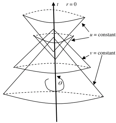
If in equation (12) the advanced and retarded null coordinates (an alternative coordinate system) are given by (figure–6);

r t

v= + , u=t−r (18)

t r = 0

u = constant

v = constant

[image:7.595.85.212.161.233.2]

Figure 6: Future and past light cones are given respectively by the null surfaces u, v = constant.

(

v≥u

)

which gives reference frame based on null cones, which is most suitable to analyze the radiation fields; then (12) becomes [4, 5];

(

)

2 2 2

4

1 _{− Ω}

+ −

= dudv u v d

ds (19)

with −∞<u<∞ and −∞<v<∞.

Now, information at future null infinity corresponds to taking limit as

v

→

∞

, which amounts to moving in future along u = constant light cones and similarly past null infinity corresponds to

u

→

∞

. Absence of 2

du and 2

dv

in (19) indicates that {u = constant} and {v = constant} are null. We can compactify the Minkowski pace-time M by means of a conformal transformation of equation (19) is given by;

(

₂

) (

1 ₂

)

1 2

1

1

+

−

+

−

=

Ω

v

u

.

From null coordinates u, v we define new null coordinates in which the infinities of v, u have been transformed to finite values. Let us introduce new coordinates p, q by v =

tanp, u = tanq with

2 2

π

π

_{< <}

− p , _.

2 2

π

π

_{< <}

− q Then

(19) becomes;

(

)

{

2 2

}

2 2 2

sin sec

sec − + − Ω

= p q dpdq p q d

ds . (20)

The light cones are unaltered after conformal transformation. Then metric

g

_µν on the unphysical

space-time M, after conformal transformations is given by;

(

)

2 2

2 2

2=₄Ω _ds =−_dpdq+_{sin p}−_{q d}Ω s

7

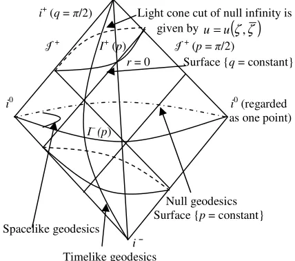
It is seen that equation (21) is a manifold embedded as a part of the Einstein static universe. To see this let;

i+ (q = π/2) Light cone cut of null infinity is given by u=u

( )

ζ,ζ I +

I+ (p) I +

(p = π/2)

r = 0 Surface {q = constant}

i0 i0 (regarded as one point) I– (p)

Null geodesics Surface {p = constant} Spacelike geodesics

i –

[image:8.595.67.281.151.340.2]

Timelike geodesics

Figure 7: Conformal infinity in the Minkowski space-time.

q p

T= + , R=p−q (22)

where −

π

<T+R<

π

and −π<T−R<π, R > 0 then (22) becomes in

(

T

,

R

,

θ

,

φ

)

as;

2 2 2 2 2

sin

Ω

+

+

−

=

dT

dR

R

d

ds

. (23)

This is a natural Lorentz metric

S

3

×

ℜ

which is the Einstein static universe [1]. Then future null infinity is given by T=π−R for

0

<

R

<

π

and the past null infinity is given by T=−

π

+R for

0

<

R

<

π

. Let us introduce complex stereographic coordinates ζ and its

complex conjugate ζ such that u=u

( )

ζ

,

ζ

on the sphere are defined by;

θ ζ φ 2 1 cot i e

= , _ζ φ _θ

2 1 cot i e− =       − −

= θ θ θ φ

ζ _eφ _{ec d i d}

d i 2 1 cot 2 1 cos 2 1 2       + −

= − _{θ θ θ φ}

ζ φ d i d ec e d i 2 1 cot 2 1 cos 2 1 2 θ ζ ζ 2 1 cos 4 1 2

1 2 4

0 2 ec P = =       ₊ 2 2 2 2 0

sin θ φ θ ζ ζ d d P d d + = .

Hence (23) becomes 2 0 2 2 2 2 P d d r dudr du

ds =− − +

ζ

ζ

. (24)

Let us substitute u= 2u′,

r

2 1

=

l and the conformal

factor is

Ω

=

₂

l

, then conformal transformation of (24) becomes; 2 0 2 2 2 2

2 _{4 4}

P d d d u d u d ds s

d =Ω =− l ′ + ′ l+

ζ

ζ

. (25)

Dropping the primes we get;

2 0 2 2 2 2 2 4 4 P d d dud du ds s

d =Ω =− l + l+

ζ

ζ

. (26)

If r→∞ then

l

→0 and the null infinity I + is defined by the condition l=0. Future directed null cones are characterized by the values u, _ζ and ζ, so the

coordinates

(

u

,

ζ

,

ζ

)

can be used as coordinates on I +, which are called Bondi coordinates on I +_{. In this}

coordinate system a hypersurface of I +

has the metric;

2 0 2 P d d ds =

ζ

ζ

.

Hence I + _{is a null hypersurface which is generated by the}

null curves ζ,ζ =constant. For conformal metric;

(

0,1,0,0

)

= ∂ Ω ∂ µ x

and ₌₀

∂ Ω ∂ ∂ Ω ∂ ν µ µν x x

g on I +. (27)

Hence Ω is differentiable on M, the new unphysical manifold with boundary and

µ

x

∂ Ω

∂ _{is a null vector. Ω is}

smooth everywhere and Ω=0 at I +, which is a null hypersurface.

Now, we will discuss the complete light cone at any given apex point in the space-time. All the known null geodesic equations of the space-time are given by [2];

1 2

_l

2_u

_&

−

_l

&

=

,

0

2

=

+

u

u

&

&

l

&

_,

(

1

₊

ζ

ζ

)

₋

2

ζ

ζ

2

₌

0

8

(

1

+

ζ

ζ

)

−

2

ζ

ζ

2

=

0

ζ

&

&

_&

&

,

0

4

4

₂

0 2

2

₋

₋

₌

P

u

u

ζ

ζ

&

&

l

&

&

&

l

.

Here dot denotes derivative with respect to affine parameter s. The last equation of (28) correspond to

0

2

=

ds

. For simplicity let us consider the equation for the

equatorial plane

2

π

θ

=

then

ζ

=

e

iφ. Now we write;

( )

φ

ζ

&

φ

&

i

e

i

=

,

ζ

&

&

=

e

iφ

(

i

φ

&

&

−

φ

&

2

)

,

(

)

2

φ

φ

ζ

&

&

₌

_e

−iφ

₋

_i

&

&

₋

&

.

The third equation of (28) gives,

φ

&&=0,

φ

&=b.

The first equation of (28) gives,

2

2

1

l

l

&

&

=

+

u

.

The last equation of (28) gives, _1−l&2_=l2_b2_.

2 2

1 b ds

d

l l

l

&_{= =± −}

∴

2 2

1 b d ds

l l

− ± =

∴ . (29)

If l&<0 then a null ray moves away from the origin, if

0

>

l

&

then the ray moves away initially towards the origin of the coordinate system

(

_r=_0,l=∞

)

and after reaching a maximum value r_m where

=

1

−

2 2

=

0

m

b

l

l

&

_{, it begins}

to move outwards and again l&<0. We have [2, 4],

2 2

1 b bd bds

d

l l

− − = =

φ

. (30)

ds d ds

du l

l

l ₂ .

1 2

1

2 2 +

=

2 2 2

2 _{1 2}

2 l

l l

l

l d

b d

du +

− −

= . (31)

At apex of the cone,l=l₀,

u

=

u

₀and

φ

=

φ

₀. Then, integrating the above equations from l₀ to an arbitrary

l

we find the equations for one sheet of the light cone. For simplicity let us choose at apex

l

=

0

,

φ

₀

=

0

. Integrating (30) and (31) we get;

0 2 0 2 0

2 1 1

l l

b u

u= + − − . (32)

( )

0 1

sin− bl

=

φ

.

Initial direction b ranges from 0 to

l

−₀1. Note that for a

fixed apex one has a one-one relation between the initial direction b and the final angular position φ on the future null infinity. By eliminating b from above equations we obtain the equatorial plane portion of the light cone cut which is given by;

(

1

cos

φ

)

2

1

0

0

+

−

=

l

u

u

. (33)

For the sheet l&<0, cos is positive and φ l&>0,

cos

φ

is negative. Here we have considered only equatorial plane, so (33) describes only on 1

S _{worth of null rays, as we have}

null rays intersection I +

, since we have restricted ourselves to the equatorial plane. For spherically symmetry the full cut, which is topologically _S2_{, can be generated by rotating}

this plane.

Conclusions

In this paper we have tried to give a simple explanation of the Minkowski geometry. Before discuss Minkowski geometry we have tried to explain briefly the general relativity, differential geometry and some necessary definitions. Thinking about the common readers, we have avoided complex mathematical calculations. First we have discussed the differentiable manifold, space-time manifold, topology and space-time causality conditions. Then we also have briefly discussed the Einstein equations and related symbols with these equations. We have stressed on the description of the Minkowski geometry and have tried our best to explain it clearly. We have added diagrams to clarify the descriptions and concepts of the paper to the readers.

References

1- Hawking S.W., Ellis, G.F.R., The Large Scale Structure of Space-time, Cambridge University Press, Cambridge. 1973.

2- Joshi P.S., Global Aspects in Gravitation and Cosmology, Clarendon Press, Oxford. 1993.

3- Lipschutz, S., General Topology, Schum’s Outline Series, Singapore, 1st edition, 1965.

4- Mohajan H.K., Singularity Theorems in General Relativity, M. Phil. Dissertation, Lambert Academic Publishing,Germany. 2013.