Decoding Solar Wind–Magnetosphere Coupling
M. J. Beharrell,
1F. Honary,
1Abstract.
We employ a new NARMAX (Non-linear Auto-Regressive Moving Average with eX-ogenous inputs) code to disentangle the time varying relationship between the solar wind and SYM-H. The NARMAX method has previously been used to formulate a Dst model, using a preselected solar wind coupling function. In this work, which uses the higher res-olution SYM-H in place of Dst, we are able to reveal the individual components of dif-ferent solar wind-magnetosphere interaction processes as they contribute to the geomag-netic disturbance. This is achieved with a GPU-based NARMAX code that is around ten orders of magnitude faster than previous efforts from 2005, before general-purpose programming on GPUs was possible. The algorithm includes a composite cost function, to minimize over-fitting, and iterative re-orthogonalization, which reduces computational errors in the most critical calculations by a factor of ∼106. The results show that neg-ative deviations in SYM-H following southward IMF are firstly a measure of the increased magnetic flux in the geomagnetic tail, observed with a delay of 20-30 minutes from the time solar wind hits the bow shock. This piling up of magnetic flux corresponds to the substorm growth phase. Terms with longer delays are found which represent the dipo-larization of the magnetotail, the injections of particles into the ring current, and their subsequent loss by flowout through the dayside magnetopause. Our results also indicate that the contribution of magnetopause currents to the storm time indices do not only depend on solar wind dynamic pressure, but also increase with solar wind electric field,
E = v×B. This is in agreement with previous studies that have shown the magne-topause is closer to the earth when the IMF is in the tangential direction.
1. Introduction
The interaction of the solar wind and earth’s magneto-sphere, beginning when an element of the solar wind im-pacts the dayside magnetopause, is a process that lasts sev-eral hours, evolving as the solar wind progresses around the magnetosphere. On the nightside, particles are injected into the ring current and accelerated as the magnetic field dipo-larizes. The populations of these particles subsequently de-cay in a number of ways, including charge exchange with the upper atmosphere (particle precipitation) and flowout from the dusk and dayside magnetopause. Each stage of the interaction has a unique effect on Dst, a measure of the geomagnetic disturbance field on Earth.
There can be no doubt that the populations of energetic particles in the inner magnetosphere are enhanced during geomagnetic storms, nor that these particles contribute to negative excursions of the Dst index. To a first approxima-tion the magnetic effect of the particles can be calculated with the Dessler-Parker-Sckopke (D-P-S) relation [Dessler and Parker, 1959;Sckopke, 1966], which is written in mod-ern terms as
µ·b(0) = 2UK, (1)
where b(0) is the (vector) average disturbance field over the surface of the earth, µ is the dipole moment, and UK
is the total kinetic energy of the plasma in the magneto-sphere. The particles are primarily injected and accelerated on the nightside, as the tail magnetic field reconnects and relaxes to a more dipolar configuration. Traditionally a mag-netic storm is considered to be a rapid succession of these
1Physics Department, Lancaster University, UK. LA1
4WA.
Copyright 2016 by the American Geophysical Union.
dipolarization-injection events, which are called substorms. However, the findings ofIyemori and Rao [1996] appear to contradict this picture. They report that the Dst index de-cays (becomes less negative) after substorm onset. Siscoe and Petschek [1997] provides an explanation: during sub-storm onset the magnetic energy contained in the stretched magnetotail is transferred to charged particles in the ring current, but the stretched magnetotail itself has a Dst con-tribution, which is reduced during dipolarization. Further evidence of this is provided byLopez et al.[2015], who report that, during the magnetic storm of 31 March 2001, SYM-H was observed to decrease by more than 200 nT without any ring current enhancement, but with growth of the magneto-tail. During the storm, a large injection also coincided with a positive change (loss) in SYM-H. EarlierSiscoe[1970] had extended the D-P-S relation to include the magnetic field energyUb,
µ·b(0) = 2UK+Ub, (2)
The influence of the ring current kinetic energy on the dis-turbance field is twice that of the magnetic energy. This means that when the magnetotail dipolarizes, and magnetic energy from the tail is transferred to the ring current, there will be a decay in the Dst index if more than half of the magnetotail energy is lost elsewhere. On the other hand, if more than 50% of the energy stored in the tail is trans-ferred to the ring current there will be an increase in -Dst. A substantial part of the magnetic energy transferred from the solar wind in the merging, convecting, and separating of the geomagnetic field and the IMF is lost downstream as a plasmoid during the substorm expansion process, and as Joule heating in the ionosphere.Wang et al.[2014] estimate that 13% of the solar wind kinetic energy is transferred to the magnetosphere. The input energy is roughly equally di-vided between the auroral ionosphere, the ring current, and the plasmoid [Ieda et al., 1998; Kamide and Baumjohann, 1993]. The portion of energy that remains in the enhanced
ring current persists and builds up over the course of a geo-magnetic storm.
Typically, the first change seen in Dst at the beginning of a storm is a positive swing, due to an increase in the dayside magnetopause current from an enhanced solar wind dynamic pressure. The injection of energetic particles into the ring current, resulting in prolonged negative Dst values, occurs primarily on the nightside. It takes time, of the order of an hour, for newly merged IMF and geomagnetic field lines to convect to the nightside of the planet and diffuse through the magnetotail, at which point the open geomagnetic field reconnects (closes), and undergoes dipolarization. Many for-mula are available that describe the negative excursions of Dst in terms of the solar wind parameters, some of these are listed in section 5. These “coupling functions” are often (incorrectly) assumed to directly represent the rate of par-ticle injection into the ring current, but it is no coincidence that the functions appear to describe the rate of magnetic field merging on the dayside. Following the explanation of Siscoe and Petschek[1997], the merging of magnetic flux on the dayside results in a negative swing in Dst firstly due to the deformation of the magnetotail, and the enhanced cross-tail current. Around an hour later, when this merged flux reconnects on the nightside, the injection of particles into the ring current offsets the loss of Dst from the restored geomagnetic field. At this point the negative Dst contribu-tion is transferred from the magnetic field to an enhanced ring current. Recently Vasyli¯unas [2006] points out that the deformation of the geomagnetic tail can be represented by the amount of open (merged) magnetic flux, which is largely piled up in the magnetotail. If during tail reconnec-tion the gain in -Dst from the ring current exactly cancels the loss from the reduced magnetotail contribution, then the coupling functions, which describe the enhancement of -Dst over the course of a storm, will be identical to the rate of dayside magnetic field merging. However, there is no rea-son to believe that exactly half of the magnetotail energy is transferred to the ring current, so that its contribution to Dst exactly replaces that of the deformed magnetotail.
The low time resolution of Dst has no doubt hampered past efforts to examine the coupling processes in detail. By using the higher resolution, but otherwise equivalent SYM-H [Wanliss and Showalter, 2006], we aim to discover formula describing changes in the disturbance magnetic field for each of the mechanisms described in this section. These include the magnetopause currents, magnetotail currents, magne-totail reconnection and particle injection, flowout through the magnetopause, and atmospheric charge exchange losses. To this end, we employ a new NARMAX code (Non-linear Auto-Regressive Moving Average with eXogenous inputs). NARMAX has previously been used to formulate a 1-hour resolution Dst model, using a preselected coupling function [Boynton et al., 2011a]. The choice of coupling function, (de-scribed in Boynton et al.[2011b],) is made using the OLS-ERR (Ordinary Least Squares – Error Reduction Ratio) al-gorithm. OLS-ERR is commonly used to select NARMAX model terms; here it was used to choose between approxi-mately 3600 candidate coupling functions. While the Boyn-ton et al. [2011a] model provides a good approximation to Dst, the use of a single coupling function at 1-hour time res-olution suggests that the function represents a mixture of the various coupling processes.
2. Theory
Some important physical processes in solar wind – mag-netosphere coupling occur in timescales shorter than the 1 hour resolution of the Dst index. To pick apart the dif-ferent mechanisms it is necessary to use the higher resolu-tion SYM-H index. SYM-H is equivalent to Dst, but sam-pled at 1 minute resolution [Wanliss and Showalter, 2006]. The Burton-Mcpherron-Russell continuity equations for Dst
[Burton et al., 1975] can therefore be written in terms of SYM-H.
SYM-H∗= SYM-H−b√p+c, (3)
d SYM-H∗ dt =Q−
SYM-H∗
τ , (4)
where SYM-H∗is a pressure-corrected SYM-H, ie with the Chapman-Ferraro (magnetopause) currents removed. To a first approximationb is usually assumed to be a constant, its value determined by the geometry of the dayside mag-netopause. c is also assumed to be a constant. Q is a source term representing the injection of charged particles into the ring current, and SYM-H∗/τ represents an ideal-ized exponential decay of the ring current. More recently it has become apparent that other important terms exist, and these should be added to the SYM-H continuity equa-tion. Flowout, where particles entering the magnetosphere on quasi-trapped orbits drift out of the dayside magne-topause, is especially significant during storms [Kozyra and Liemohn, 2003]. Changes observed in Dst that are associ-ated with the well known solar wind coupling functions, are commonly but incorrectly thought to be a direct measure-ment ofQ, the injection of particles into the ring current. Vasyli¯unas [2006] points out that the effects described by the coupling function are firstly due to the increasing mag-netic flux in the magnetotail. Therefore, Dst and SYM-H must depend on the flux of open geomagnetic field lines, the majority of which are piled up in the magnetotail. The total rate of change of open magnetic flux can be written as the opening rate of flux on the dayside, minus the closing rate on the nightside.
d SYM-H∗
dt =Q+F−
SYM-H∗
τ −a
d Φd dt −
d Φn dt
, (5)
where the coefficient a provides the conversion from mag-netic flux in the tail to SYM-H on the ground; d Φd
dt is the rate of flux opening on the dayside and piling up in the tail, and d Φn
dt is the rate of flux closing in nightside reconnection. F is the rate of flowout from the dayside magnetopause. Note that the sign ofQis negative, as particles entering the magnetosphere increase -SYM-H, whereasF is positive.
Equation 5 is converted to use discrete time steps, ∆t, and SYM-H is substituted for SYM-H∗using equation 3,
SYM-H−B−1=
1−∆t τ
(SYM-H−1−B−1) (6a)
+b∆√p (6b)
−a∆Φd (6c)
+ (a∆Φn+Q∆t) (6d)
+F∆t, (6e)
based on the solar wind parameters to represent each of the terms 6a to 6e.
∆Φnis the amount of magnetic flux closed by magnetic
reconnection on the nightside during the interval ∆t. In equation 6 it is placed withQ, the injection of particles into the ring current, because both processes occur simultane-ously and are difficult or impossible to separate empirically with analysis of solar wind and SYM-H data.
The physical processes linking variations in the solar wind to changes in SYM-H, such as the merging of flux on the dayside (∆Φd), and nightside (∆Φn), and enhancements in
magnetopause currents (∆√p) each have different delays, or lags, relative to the arrival time of solar wind at the bow shock. For example, an increase in solar wind dynamic pres-sure results in an almost instantaneous increase in SYM-H, due to the magnetopause currents, but the closing of mag-netic field lines on the nightside and accompanying injection of particles can lag by tens of minutes, as the magnetic field lines must first convect around the planet and diffuse into the tail. The differences in the lag times are exploited by the NARMAX model selection technique to decode the time series of SYM-H and solar wind data. In this paper a fast NARMAX code is used to find functions of solar wind pa-rameters that best represent each of the 5 terms in equation 6.
3. Data
The solar wind data we use, spanning 1 January 1995 – 1 June 2013, is taken directly from the OMNI2 data set [King and Papitashvili, 2005]. Although solar wind data is available from as early as the 1960’s, in an attempt to avoid possible bias from the varying sources we use only data from after 1995, which is provided by the newer ACE and WIND spacecraft. This has the additional benefit of reducing the size of the data set and speeding up the calculations. Data between 17 March 2000 and 9 May 2000 is excluded. This is a period with few data gaps, and is therefore ideal for val-idating the model. The OMNI2 magnetic field and plasma data has been time shifted to compensate for the location of the spacecraft, which are approximately 1 hour upstream of the Earth. The solar wind data is combined with SYM-H, and integrated to 5 minute samples.
It is advantageous to run the NARMAX algorithm on multiple subsets of the data. Comparing the results ob-tained for each subset shows the level of consistency of the model results, and reveals any over-fitting. Splitting the data set requires some care. If the data are split at a partic-ular epoch there may be a bias in the results if, for example, the earlier data set is recorded during a different part of the solar cycle, or during a different season to the latter part of the data set. Separating the data set on a sample-by-sample basis is also problematic, as neighboring samples will be far from independent, and the two data sets will be nearly iden-tical. Instead, the data is grouped into week-long segments, each containing 2016 samples (5 minute resolution). The week long segments are randomly distributed between two data sets: a training set, and a testing set. This method gives two independent and unbiased data sets, which are made as close in size as possible. The NARMAX algorithm is run on one of the two halves of data, while the other half is used to check the quality of the result as each term is selected. The model result is labeled ‘1A’. Next, the two subsets of data are switched around, with the training set becoming the testing set, and vice versa, and the result is labeled ‘1B’. The results 1A and 1B are based on separate data sets, ie no samples are used by the NARMAX code for both models 1A and 1B. The data randomization procedure is repeated, with the week-long segments again being dis-tributed randomly between two new subsets of data. This time the results are labeled 2A and 2B. While 2A and 2B are produced using separate data sets, there is some overlap between the data used for 1A and 2B, for example. The pro-cedure is repeated 5 times, giving a total of 10 NARMAX model results for comparison.
4. The NARMAX technique
The goal of the NARMAX method is to produce a model for a response variable,y(t), in the form
y(t) =
M
X
k=1
pk(t)θk+ξ(t), (7)
wheretis the sample number (1,2,...,N),pk(t) is thekth
pre-dictor out of a total ofM, andθk is the coefficient of that
predictor. ξ(t) is the uncorrelated model residual, ie the part ofy(t) that cannot be represented by any of the pre-dictor terms. In our case the outputy(t) = SYM-H∗(t), and each of theM predictor terms is a different product of the various solar wind parameters and SYM-H∗values, with a range of lag times. For example, one of the parameters could be density×pressure at a lag of 10 minutes, and another could be SYM-H∗2 ×pressure2 with a 15 minute lag. The NARMAX method seeks to identify themmost important predictors, (typically between 5 and 20,) and provide their coefficients. The number of candidate predictor terms,M, can clearly be very large when there are more than a few lags and solar wind parameters, so the candidates are lim-ited to a particular degree of non-linearity (the sum of all of the powers in the product).
Simply ordering the candidate predictor terms by their correlation withy(t), and selecting the topm, generally does a very poor job of model selection. With this naive approach the selected terms will tend to be strongly correlated with each other, and each will add very little additional infor-mation to the model. To produce an effective and efficient model it is far better to select predictors that each represent a unique aspect of the response variable. In other words, each variable should be selected based on the information it contains that is not present in any of the other selected terms. The NARMAX method achieves this by orthogo-nalizing the candidate predictor vectors,pkwith respect to
the previously selected and orthogonalized predictor vectors, w1,w2, ...,wk−1.
In vectorized form, equation 7 can be written as
y=PΘ+Ξ (8)
wherePis a matrix formed by the candidate predictor vec-tors, withMcolumns andNrows. Θis the vector of coeffi-cients.Pcan be decomposed into a product of an orthogonal matrixW, and an upper triangle matrixA.
P=WA (9)
where,
W=
w1(1) w2(1) w3(1) . . . wM(1)
w1(2) w2(2) w3(2) . . . wM(2)
. .
. ... ... . .. ... w1(N) w2(N) w3(N) . . . wM(N)
(10)
Every column ofWis orthogonal to every other column, and each is a vector, wk, representing a time series of the
kth variable. It is not practical or necessary to compute the full orthogonal matrixW, instead only the firstmcolumns are filled with thewk vectors that correspond to the best
NARMAX algorithm according to the value of the error re-duction ratio, [ERR]k,
[ERR]k= (w
T ky)2
wT
kwk yTy
. (11)
At thekth selection, the remaining candidates are each or-thogonalized relative to the previously selected basis vectors, w1,w2, ...,wk−1. The candidate with the largest [ERR]kis
selected to be thekth parameter. The selection process can be terminated when a desired tolerance,ρ, is reached
1−
m
X
k=1
[ERR]k< ρ. (12)
For a more complete description of the NARMAX model selection technique see eg Billings [2013] To improve the accuracy of the orthogonalization calculations in the NAR-MAX algorithm, iterative reorthogonalization [Hoffmann, 1989] is implemented, to ensure that the selected orthogo-nal vectors, wk, are precisely orthogonal. Testing showed
this to produce an improvement in orthogonality of a factor of around 105 to 106, enabling the code to select the best terms even where there is a high level of ill conditioning.
0 1 2 3 4 5 6
1e 7
0.0 0.2 0.4 0.6 0.8 1.0
[image:4.595.76.288.328.510.2]BIC relative likelihood
Figure 1. BIC derived relative likelihood of each
NAR-MAX result, using data set 2A, as a function of the cost functionα.
In an attempt to minimize over-fitting, a composite cost function is employed following the method ofHong and Har-ris[2001]. Its purpose is to penalize covariance between the selected parameters and minimize model prediction errors. The cost function, α, is a small positive scalar parameter that balances the model’s approximation capability against its tendency to over fit the data. Instead of maximizing ERR, we maximize
ERR−α
N
wT
kwk yTy
. (13)
When α= 0 the algorithm is the identical to the more typical ordinary least squares ERR method. The NARMAX model selection is terminated when there are no more can-didate predictors for which expression 13 is positive. Large αleads to no predictors being selected at all, since all are judged to have too high a variance. AlthoughHong and Har-ris[2001] do not provide a way to to automatically choose a reasonable value forα, it is possible to search all ofα-space
for the best result, since a range of α values will produce exactly the same NARMAX model. This is achieved by running the NARMAX code firstly withα= 0, then with the smallest value ofα, greater than the current value, that would produce a different model result. For each candidate predictor term, pk, that was not selected, a corresponding
αkis calculated. αkis the minimum value of αthat would
lead topkbeing the chosen regressor. Theαkthat is closest
to the currentαis used for the next iteration of the model. For our data set it typically requires 15 to 20 values ofα to cover the whole ofα-space, from 0 to the value of αfor which no terms are selected for the model.
The NARMAX code was implemented in OpenCL, and run on a single AMD Radeon R9 290X graphics card. OpenCL allows the algorithm to be programmed at a low level, with efficient use of the 2,816 stream processors, reg-isters, caches, and 4 GB of on-board RAM. The code scales well, with each model run in this paper taking 1 to 14 hours. Extrapolating the CPU times given by Billings and Wei [2005] (their table 1) suggests a CPU time of the order of tens of millions of years to complete a single model run of the current work. Of course, some of this speed up, perhaps a factor of 1000×, is due to today’s availability of fast and highly parallel GPUs, and the overall advances in computer performance over the last decade.
5. Parameter choices for model selection
The measurement parameters utilized in the NARMAX model are carefully chosen to ensure that the predictor vari-ables are capable of reproducing equation 6. In order to accurately and precisely determine the unknown functions in the equation, a large range of exponents with small in-tervals are required in the candidate terms. The chosen measurement parameters are:
|SYM-H∗|1/2
∆√p, p1/3, p1/12, p−1/2
n3/2, n1/3, n1/12
E1/2, E1/3, E1/12
sinθ 2,sin
4θ
2, (14)
whereE(=vBT), used throughout this paper, is the solar
wind electric field in units of mV·m−1;pis the dynamic so-lar wind pressure in nPa;nis the solar wind proton number density in cm−3; andθ is the IMF clock angle.
Lags of the solar wind parameters, ranging from 5 minutes to 4 hours, are added to the data set. To reduce computa-tion time the longer lags are spaced at intervals. 5 to 60 minute lags are spaced at 5 minute intervals (i.e. without gaps), 60 to 120 minute lags are spaced at 10 minute inter-vals, and lags greater than 2 hours are spaced at 15 minute intervals.
Products of these parameters form the predictors in the NARMAX model, which are constructed up to a non-linearity degree of 8. In other words, each candidate term in the NARMAX model comprises up to 8 of the measurement parameters multiplied together, with the same parameter able to appear more than once in each term. In forming the candidate predictor terms only solar wind parameters with the same lag are included in each term. A single 5 minute lag of the|SYM-H∗|1/2
parameter is included. This is com-bined in the candidate terms with solar wind parameters of any lag. For example, one of the candidate predictors will be [|SYM-H∗|1/2
(t−5 m)]3·[
In total there are 4,770,710 candidate predictors, including a constant term.
The NARMAX algorithm does not work with missing data, so any samples that contain missing data (in any of the lags from 0 minutes to 4 hours) are excluded. The remaining data comprises 1,175,732 samples.
Some examples of previously suggested coupling functions that are included in the candidate terms, with each of the aforementioned lags, are:
• Kan and Lee [1979]: vBTsin2θ2 =E1/2·E1/2·sinθ2 ·
sinθ
2 (non-linearity degree 4) • Wygant et al.[1983]: vBTsin4θ2
• Scurry and Russell [1991]: vBTsin4 θ2p1/2
• Temerin and Li [2006]: n1/2v2BTsin6 θ2
These and many other variations of the coupling func-tions could be selected by NARMAX to be included in the model’s approximation of equation 6. Similarly, the algo-rithm is able to choose different functions of the solar wind parameters for the other terms in equation 6. For example, if the coefficientbis better approximated by one of these func-tions, instead of a constant, that function will be selected. If the true Chapman Ferraro term is proportional to ∆√3p, instead of ∆√p, the model is able to select ∆√p·p−1/2·p1/3 as a close approximation.
6. Results
The NARMAX selected model terms for the first run of the algorithm, 1A, are given in table 1. The first se-lected predictor term is 0.9945 SYM-H∗(t−5 m). A model containing only this single term would be SYM-H∗(t) = 0.9945 SYM-H∗(t−5 m), which describes an exponential decay of SYM-H∗, with a time constant of 15.1 hours. To a first approximation this model describes the decay of the ring current in the absence of energy input from the solar wind.
The standard method of measuring the significance of a term in NARMAX is with the Error Reduction Ratio (ERR). The higher the ERR value of a term, the closer it will allow the model to fit the data. The sum of ERR values approaches 1 as the the model becomes more complicated and fits the data more precisely. However, at some point the model will likely become over-fitted as new model terms are fitting to measurement errors instead of real physical processes. To address this, the relative likelihood of each term is calculated from the Bayesian Information Criterion (BIC), using the testing half of the data set, which is as-sumed to be independent of the training data used by the NARMAX code. The cumulative ERR, and relative likeli-hood at each step of the model selection are given in table
1. They indicate that the most likely model has 11 terms, with subsequent terms leading to over-fitting.
The composite cost function ofHong and Harris [2001] was employed, and the model was computed with a number of different values of the cost function,α. In all but one of our model runs, the model withα= 0 provides the best fit to the testing data set, according the BIC. The single run that was improved with a non-zero cost function was run 2A. The relative likelihood of the models of run 2A, as a function ofα, are shown in figure 1. Composite cost func-tions are an effective means of reducing over-fitting, and the reason they are not especially helpful here is because the data sets are large (∼600,000 samples, compared to 100 in the example given byHong and Harris [2001]).
Of course, each 5 minute sample is not entirely indepen-dent of its neighbors. When calculating all BIC values an ef-fective number of independent observations is used. Follow-ingZieba[2010], this is calculated using the auto-correlation of SYM-H as 1
50 th
of the number of samples.
Most of the terms given in table 1 begin to look very fa-miliar, as almost identical terms are seen in each of the 10 NARMAX runs. The terms are described briefly below, and in more detail in the next section.
The second most significant term chosen by the NAR-MAX algorithm has a positive coefficient, short lag time, and contains ∆√p. These properties, which are also shared with terms 4 and 8, are associated with the Chapman-Ferraro (magnetopause) currents, corresponding to part b of equation 6.
Terms 3, 6, and 10 resemble the coupling functions listed in the previous section. They are functions ofE and sinθ2, with negative coefficients, and lag times that are consistent with the time it takes solar wind to transverse the mag-netosphere, and pile up in the magnetotail. The negative coefficients means that an enhancement in the IMF – mag-netosphere dayside merging rate will result in larger negative SYM-H values 20 to 30 minutes later. These terms represent part c of equation 6.
The fifth term appears to be essentially the geometric mean of the first term (a decay term) and the coupling function terms. The lag time associated with the coupling component is 90 minutes, which is approximately the time it takes merged magnetic field lines to transverse the mag-netosphere, diffuse through the magnetotail and begin to reconnect. We associate this term with the loss of SYM-H as the open magnetic field in the magnetotail reconnects, injecting particles into the ring current. In this process en-ergy is lost primarily by Joule heating in the ionosphere and in the plasmoid escaping down wind. This term represents part d of equation 6.
[image:5.595.137.489.614.757.2]We are unable to attribute term 7 to any physical pro-cess. The decrease in the model’s relative likelihood with
Table 1. Results from run 1A of the NARMAX code. The 11-term model has the highest likelihood, calculated
by comparing the model results at each stage against a separate data set, using the Bayesian Information Criterion.
Term Coefficient Chosen parameters Cumulative Relative
(lag times in parentheses) ERR likelihood
1 +0.9945 SYM-H∗(5 m) 0.99840838 9.0×10−541
2 +1.662 ∆√p E1/3n2/3p−1/2(5 m) 0.99853963 3.5×10−374
3 −0.1220 E3/4p1/3sin5θ
2(25 m) 0.99864883 6.0×10
−211
4 +2.477 ∆√p E1/3p1/12(0 m) 0.99874214 8.8×10−49
5 +0.03593 |SYM-H∗|1/2(5 m)E1/3p1/4sin2θ
2(90 m) 0.99875181 1.6×10
−33
6 −0.1598 E5/6p1/3sin4θ
2(20 m) 0.99875788 6.7×10
−18
7 −0.001384 |SYM-H∗|1/2∆√p E11/12n3/2p−1/2sinθ
2(5 m) 0.99876334 1.5×10
−18
8 +0.2777 ∆√p n3/2p−23/12(10 m) 0.99876845 2.7×10⁻¹⁰
9 −0.1789 ∆√p E5/6n2/3p−1/2sin2θ
2(15 m) 0.99877286 1.1×10
−7
10 −0.1184 E11/12n1/3p−1/6sin5θ
2(30 m) 0.99877599 6.8×10
−6
11 +0.05670 En1/2p−1/2sin5 θ
2(150 m) 0.99877983 1
Table 2. NARMAX model terms associated with solar wind dynamic pressure. These terms represent part b of equation 6.
Run 0 minute lag 5 minute lag 10 minute lag
1A +2.477E1/3p1/12∆√p +1.662E1/3n2/3p−1/2∆√p +2.777×10⁻¹n3/2p−23/12∆√p
1B +2.115E1/2∆√p +1.472E1/2n2/3p−2/3∆√p +1.498×10⁻¹n11/6p−2∆√p
2A +2.080E5/12p1/12∆√p +1.546E1/2n2/3p−2/3∆√p +2.571×10⁻¹n3/2p−11/6∆√p
2B +2.803E1/3n−1/6p1/4∆√p +1.634E1/3n2/3p−1/2∆√p +2.812×10⁻¹n3/2p−23/12∆√p
3A +2.474E5/12∆√p +1.665E5/12n2/3p−2/3∆√p +3.228×10⁻¹n3/2p−11/6∆√p
3B +2.069E5/12p1/12∆√p +1.426E1/3n2/3p−1/2∆√p +2.577×10⁻¹n3/2p−23/12∆√p
4A +2.791E1/3n−1/6p1/4∆√p +2.025E1/3n1/2p−5/12∆√p +1.690×10⁻¹n11/6p−2∆√p
4B +2.307E5/12∆√p +1.645E5/12n2/3p−2/3∆√p +3.114×10⁻¹n3/2p−23/12∆√p
5A +2.715E1/3n−1/6p1/4∆√p +1.601E5/12n2/3p−2/3∆√p +3.142×10⁻¹n3/2p−11/6∆√p
[image:6.595.83.521.231.350.2]5B +2.344E5/12∆√p +1.502E1/2n2/3p−2/3∆√p +2.738×10⁻¹n3/2p−23/12∆√p
Table 3. Traditionally referred to as coupling functions, these terms in the NARMAX model runs are associated
with the merging of the IMF and geomagnetic field (part c of equation 6). The resultant open geomagnetic field is mostly within in the tail, causing SYM-H to become more negative due to enhanced magnetotail currents.
Run 20 minute lag 25 minute lag Lags given in parentheses
1A −1.598×10⁻¹E5/6p1/3sin4θ
2 −1.220×10
−1E3/4p1/3sin5 θ
2 −1.184×10
−1E11/12n1/3p−1/6sin5θ 2(30 m)
1B −2.130×10⁻¹E3/4p1/3sin4θ
2 −1.564×10
−1E11/12n1/6sin5θ
2 −5.954×10
−2En1/3n1/3p−1/12sin5θ 2(35 m)
2A −2.429×10⁻¹E3/4p5/12sin5 θ
2 −1.423×10
−1En1/3p−1/6sin5 θ 2(30 m)
2B −1.694×10⁻¹E11/12p1/4sin52θ −2.476×10⁻¹E3/4p1/3sin4 θ2 3A −1.763×10⁻¹E5/6p1/3sin5θ
2 −1.272×10
−1E5/6p1/4sin5 θ
2 −9.254×10
−2En1/3p−1/6sin5 θ 2(30 m)
3B −2.451×10⁻¹E3/4p5/12sin5 θ
2 −1.787×10
−1E11/12n1/6sin4θ 2(30 m)
4A −2.511×10⁻¹E3/4p5/12sin5 θ
2 −1.795×10
−1E11/12n1/6sin4θ 2(30 m)
4B −1.866×10⁻¹E5/6p1/3sin5θ
2 −1.107×10
−1E3/4p1/3sin4 θ
2 −1.326×10
−1E11/12n1/6sin4θ 2(30 m)
5A −2.372×10⁻¹E3/4p5/12sin5 θ2 −1.824×10⁻¹E11/12n1/6sin4θ2(30 m) 5B −1.782×10⁻¹E5/6p1/3sin5θ
2 −2.273×10
−1E3/4p1/3sin4 θ 2
Table 4. Model terms associated with tail reconnection, the loss of magnetotail flux, and the simultaneous
injection of ring current particles. These terms represent part d of equation 6. Run Lag times given in parentheses
1A +3.593×10⁻²E1/3p1/4sin2θ 2(90 m)
p
|SYM-H∗|(5 m) 1B +2.659×10⁻²E1/2n1/6sin3θ
2(70 m) p
|SYM-H∗|(5 m) +1.857×10⁻²E5/12p1/4sin2θ 2(110 m)
p
|SYM-H∗|(5 m) 2A +1.863×10⁻²E7/12p1/6sin3 θ
2(70 m) p
|SYM-H∗|(5 m) +1.714×10⁻²E1/3p1/3sin3θ 2(90 m)
p
|SYM-H∗|(5 m) 2B +2.499×10⁻²E5/12p1/4sin2 θ
2(80 m) p
|SYM-H∗|(5 m) +2.475×10⁻²E1/3p1/3sin2θ 2(110 m)
p
|SYM-H∗|(5 m) 3A +2.680×10⁻²E5/12p1/4sin2 θ
2(80 m) p
|SYM-H∗|(5 m) +2.484×10⁻²E1/2p1/6sin3θ 2(120 m)
p
|SYM-H∗|(5 m) 3B +2.930×10⁻²E5/12p1/4sin2 θ
2(70 m) p
|SYM-H∗|(5 m) +2.307×10⁻²E1/3p1/3sin2θ 2(100 m)
p
|SYM-H∗|(5 m) 4A +2.776×10⁻²E1/3n−1/6p5/12sin2θ
2(60 m) p
|SYM-H∗|(5 m) +2.080×10⁻²E1/3p1/3sin2θ 2(90 m)
p
|SYM-H∗|(5 m) 4B +3.180×10⁻²E1/3n−1/6p5/12sin2θ
2(70 m) p
|SYM-H∗|(5 m) +2.072×10⁻²E5/12p1/4sin2θ 2(110 m)
p
|SYM-H∗|(5 m) 5A +2.670×10⁻²E5/12n1/6sin2θ
2(70 m) p
|SYM-H∗|(5 m) +1.771×10⁻²E1/3p1/3sin2θ 2(110 m)
p
|SYM-H∗|(5 m) 5B +4.136×10⁻²E1/3p1/4sin2θ
2(90 m) p
|SYM-H∗|(5 m)
the inclusion of this term indicates that it is anomalous. In other words, when this term is included the model becomes a worse fit for the testing data set.
Term 9 has a lag of 15 minutes. It represents a com-bination of two physical processes that overlap slightly in lag times: the Chapman-Ferraro current terms, with typical lags of 0 to 10 minutes; and the coupling function terms (3,6 and 10), which typically have 20 to 30 minute lag times. The overlap can be explained by the natural variation of lag times during different solar wind conditions. Lags will be short-ened when the solar wind is fast. Errors in time-shifting of OMNI solar wind data from the L1 Lagrange point to Earth orbit may also increase the spread of lag times calculated for each process.
Term 11 has the longest lag of all of the NARMAX se-lected terms, at 150 minutes. It is similar in form to the dayside magnetic field merging (coupling) terms, but it has a positive coefficient indicative of a loss term. The rate of merging of the IMF and the geomagnetic field is expected to be proportional to the subsequent, delayed, injection of particles into the ring current. These particles drift from the nightside injection region to the dayside in approximately 1 hour. The lag of this term is 60 minutes longer than that of term 5, which is associated with the injection of particles into the ring current. It is likely that this term represents
a first approximation of the flowout of ring current parti-cles through the dayside magnetopause. This is part e of equation 6.
In the next sections we discuss each of the terms in more detail, and offer explanations for their forms.
7. Discussion
Tables 2, 3, 4, and 5 list all of the identified terms in each of the model runs. The consistency of the functions found using different sets of data provides a level of confidence in the results. Note that the coefficients alone do not represent the significance of each model term, because the functions vary. Figure 2 provides a schematic of the coupling mecha-nisms associated with these terms, and shows their respec-tive lag times, relarespec-tive to the moment an element of solar wind reaches the bow shock.
7.1. Charge exchange losses
It is identified as part a of equation 6. The mean exponential time scale,τ, given by the model runs is 17.6 hours, with a standard deviation of 2.2 hours. This loss term is primar-ily associated with charge exchange between ring current particles and the upper atmosphere, because, unlike other identified loss mechanisms described later, the rate of charge exchange depends on the overall number of particles in the ring current.
PDYN
(i) 0 m
(ii) 5 m
(iii) 25 m
(iv) 90 m
(v) 90 m
(vi) 150 m
Figure 2. Schematic showing the physical processes
identified in the NARMAX model terms, with the typ-ical lag times. (i) An element of solar wind arrives at the dayside magnetopause. (ii) The IMF in that element merges with the geomagnetic field, while the solar wind dynamic pressure temporarily contributes to SYM-H via Chapman Ferraro currents. (iii) Open geomagnetic field piles up in the magnetotail, enhancing the tail current and -SYM-H. (iv) The open geomagnetic field has dif-fused throught the magnetotail and begins to reconnect. (v) Charged particles are injected into the ring current, as the magnetotail dipolarizes and the cross-tail current decays. Energy is lost from the magnetosphere in the plasmoid traveling down wind, and by ionospheric Joule heating. (vi) An hour after the ring current particles are injected from the magnetotail they reach the dayside, where those on pseudo-trapped orbits escape through the magnetopause, causing -SYM-H to decay.
Table 5. Model terms identified as ring current losses due to
flowout. These terms appear in only 6 of the 10 model runs. They represent part e of equation 6.
Run Lag times given in parentheses 1A +5.670×10⁻²En1/2p−1/2sin5θ
2(150 m)
1B +4.189×10⁻²E13/12n1/2p−1/2sin4θ 2(135 m)
2A +5.567×10⁻²En1/2p−1/2sin5θ 2(150 m)
2B 3A 3B
4A +5.998×10⁻²En1/2p−1/2sin5θ 2(135 m)
4B +5.966×10⁻²E5/6n1/2p−1/2sin5θ 2(150 m)
5A +7.073×10⁻²Esin6θ 2(135 m)
5B
[image:7.595.75.257.168.577.2]7.2. Currents induced by solar wind pressure
Table 2 gives the model terms identified with currents produced by the solar wind dynamic pressure acting on the magnetosphere, for each of the 10 model runs. All are sig-nificant terms in the NARMAX models. They each contain ∆√p, have lags of 10 minutes or less, and the coefficients are all positive. All three of the terms from a model run, added together, represent part b of equation 6.
The 0 minute lag represents Chapman Ferraro (magne-topause) currents on the dayside magnetosphere, since this is the time when a particular element of the solar wind reaches Earth. Alongside the expected ∆√p parameter, the 0-lag terms consistently contain the electric field,E, raised to the power 1/3 to 1/2. This is not surprising because the mag-netopause is up to 1 RE closer to Earth when the IMF in oriented in the YZ plane (ie perpendicular to the solar wind velocity) [Dusik et al., 2010].
In some of the runspappears with a small positive power in the 0-lag result, indicating that ∆√pmight not be ideal, with the true power ofpbeing slightly larger than 0.5. Three of the other runs containn−1/6p1/4, which can be written as p1/12v1/3, so they contain the same small-powered pressure factor, with an additional velocity contribution. Although it appears thatvhas a greater contribution in these terms, the power ofE(= vBT) is smaller, and it is actually the
contribution fromBT that is less significant.
The 10 minute lag terms are very different to the 0 minute lags. They contain two factors,n3/2andp−2. The 10 minute lags correspond to the time it takes the solar wind to pass the Earth and begin to apply pressure to the magnetotail. It is tempting to associaten3/2 with an enhanced plasma sheet density, andp−2 with a cross-tail current that moves towards or away from Earth with the varying solar wind dynamic pressure, an effect suggested by McPherron and O’Brien[2001] to affect Dst. However, the two factors when combined are approximately equivalent to a large inverse power of velocity (v−4), meaning that this term is signifi-cantly more important when the solar wind velocity is small. It remains a possibility that≈10 minute errors in the time shifting of OMNI data during periods of low solar wind ve-locity could be responsible for the 10 minute lag terms, but if the time shifting is correct, then the above explanation is plausible. The 5 minute lag terms are simply a combination of the 0 lags and 10 minute lags.
7.3. Open magnetic flux
terms all have negative coefficients, and lags between 20 and 30 minutes. The functions closely resemble the rate of day-side merging of solar wind and geomagnetic field (see eg Vasyli¯unas [2006]). All of the properties match expected changes in SYM-H from the piling up of open magnetic flux in the magnetotail and the corresponding enhancement of the cross tail current, which results in an increase of -SYM-H.
Terms with 20 minute lags are present in every model run. They are of the form−Ex1px2sinx3θ
2, wherex1 = 9/12 to
11/12, x2 = 3/12 to 5/12, and x3 = 4 to 5. The cou-pling function of Temerin and Li [2006] can be written ET&L=Ep1/2sin6θ2, so the 20 minute lag terms are equiv-alent toET&L5/6 . At longer lag times the sameE and sinθ2 dependencies remain, but the terms contain increasing pow-ers of 1/v. These 1/vcontributions are less pronounced than in the 10 minute lag pressure terms in the previous section, and it is unclear if they are both a product of errors in the time shifting of OMNI data at low solar wind speeds.
300 250 200 150 100 50 0 50
SYMH
300 250 200 150 100 50 0 50
Model SYMH
a
1A 2A 3A 4A 5A
1B 2B 3B 4B 5B
0 10 20 30 40 50 60 70 80
Mean model pressure contribution, nT
0 10 20 30 40 50 60 70 80
Model pressure contribution, nT
b
2.0 1.5 1.0 0.5 0.0
Mean model source rate, nT/min
2.0 1.5 1.0 0.5 0.0
Model source rate, nT/min
c
0.0 0.2 0.4 0.6 0.8 1.0 1.2 1.4
Mean model loss rate, nT/min
0.0 0.2 0.4 0.6 0.8 1.0 1.2 1.4
Model loss rate, nT/min
d
0 20 40 60 80 100
Mean model loss via precipitation, %
0 20 40 60 80 100
Model loss via precipitation, %
e
0 10 20 30 40 50 60 70 80 90
Mean model loss via tail reconnection, %
0 10 20 30 40 50 60 70 80 90
Model loss via tail reconnection, %
f
0 10 20 30 40 50 60 70 80 90
Mean model loss via flowout, %
0 10 20 30 40 50 60 70 80 90
Model loss via flowout, %
[image:8.595.67.495.179.663.2]g
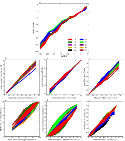
Figure 3. The variation between model runs. Panelashows the model SYM-H from each run against
7.4. Tail reconnection and particle injection
Typically around an hour after open magnetic flux enters the magnetotail, it has diffused through the tail to the point of reconnection. As the magnetic field dipolarizes following reconnection, charged particles are simultaneously injected into the ring current. This process is represented by part d of equation 6, and the associated model terms are given in table 4. Although the NARMAX model describes steady, continu-ous reconnection, in nature it tends to be bursty. The piling up of magnetic flux in the tail corresponds to the substorm growth phase, and the bursts of reconnection and particle injection are substorm expansion. The timing of substorms is very difficult, if not impossible, to predict using solar wind parameters alone, and it is not clear how much the model represents a smoothed time-average over the bursty events, or how much it represents steady tail reconnection occurring between the substorms. The increase in ring current parti-cles enhances -SYM-H, whereas the loss of magnetic flux in the tail reduces -SYM-H. According toSiscoe and Petschek [1997], the contribution to SYM-H from energy in the ring current is twice that of energy stored in the magnetotail. This means that if all of the energy stored in the magneto-tail is converted to ring current energy then -SYM-H should increase. The positive sign of the terms indicate that most of the energy is lost to other processes. This is in agreement with a statistical study of the substorm expansion energy budget byTanskanen[2002], which gives figures of 30% for each of charged particle precipitation, Joule heating, and the escaping plasmoid, with the remaining 10% going to the ring current.
The functions identified with tail reconnection appear to be the geometric means of the near-instantaneous SYM-H∗, and the dayside magnetic field merging delayed by between 60 and 120 minutes. It could be that these terms are the closest approximations, among the 4.8 million candidates, to a geometric combination of the merged flux reaching the tail reconnection point (70 to 110 minutes after merging on the dayside), and the instantaneous magnetic pressure in the tail, which is driving the reconnection. Although SYM-H∗ is itself a combination of ring current and magnetotail flux contributions, there is no better candidate term that represents only the instantaneous open magnetic flux in the tail.
7.5. Flowout
Terms in the NARMAX results identified as flowout (ta-ble 5) are the least significant among the coupling processes. They are only present in the results of 6 out of 10 runs. The functions superficially resemble the rate of magnetic field merging, but all except one depend only on the IMF, and can be written as BTsin5θ2. The lag times of 135 to 150
minutes are around an hour longer than the lag for particle injection into the ring current, which is consistent with the typical time it takes the bulk of injected particles to drift from the nightside injection region to the dayside magne-topause.
The difficulty in finding these functions with NARMAX could be because there are simply no good candidate terms that accurately describe the flowout rate. The actual flowout rate is expected to depend on the current location of the magnetopause, and the one-hour lagged charged particle in-jection rate. However, as we have seen, the rates of tail reconnection and particle injection will depend on SYM-H∗ at that time (one hour ago), and dayside merging 90 min-utes before that. Allowing multiple different lags of the solar wind parameters in each term results in far too many candi-dates than can be processed by the NARMAX code in any reasonable amount of time.
7.6. Division of energy between loss processes
Over long timescales (ie the whole data set), approxi-mately 49% of the overall loss of SYM-H in the NARMAX model is due to the terms identified with tail-reconnection,
34% to particle precipitation, and the remaining 17% from terms that appear to represent flowout. These losses are of SYM-H, not energy, and when estimating the transfer of energy, the factor of 2 in equation 2 must be taken into account. The 49% loss in SYM-H from tail-reconnection translates to a 74.5% loss in energy, primarily to the escap-ing plasmoid and Joule heatescap-ing. This is roughly consistent withIeda et al.[1998];Kamide and Baumjohann[1993], who suggest approximate equipatition of energy between the ring current, the escaping plasmoid, and ionospheric Joule heat-ing. Of the remaining 25.5% of the energy that enters the ring current, around a third (8.5%) is lost via the flowout terms, and two-thirds (17%) to particle precipitation. The loss due to particle precipitation is in line with a previous estimate of 12% byWang et al.[2014].
7.7. Variability between model runs
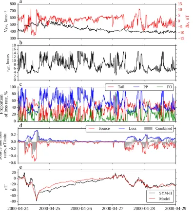
To estimate the robustness of the results the NARMAX model was run 10 times, each time varying the selection of input data (see section 3). Figure 3 shows the relative mag-nitudes of the model terms for each model run, along with the overall accuracy of each model in reproducing the ob-served SYM-H. The data used in figure 3 are from 17 March 2000 to 9 May 2000, a period that was entirely excluded from the NARMAX algorithm in all of the model runs.
Figure 3a shows the ability of the model to predict SYM-H using only the measured solar wind parameters. The model SYM-H is calculated in an iterative manner, using previousmodelvalues of SYM-H with actual solar wind mea-surements, in the NARMAX model terms (table 1). In figure 3a the model samples are binned according to the SYM-H observations, with no less than 12 samples per bin. The colored patches represent the central 50% of the model sam-ples in each bin. There is little difference between each of the models, especially at small to moderate -SYM-H where there are many samples. During these months in the spring of 2000, the models appear to systematically underestimate larger -SYM-H, but most of these samples occur in the de-clining phase of a single storm on the 6 April 2000 (see figure 4).
Figure 3b shows the variation in the magnetopause cur-rent terms of each model run. Run 1B produces a slightly smaller estimate of the magnetopause current contribution to SYM-H, but the narrow distributions (thin patches) in-dicate that the differences between model runs is primarily a scaling factor.
Figures 3c and 3d show the overall source and loss terms. The source terms are those associated with the magnetic field merging on the dayside (table 3), while the loss terms include particle precipitation (corresponding toτ in equa-tion 6), tail reconnecequa-tion (table 4), and flowout (table 5). The individual loss processes are broken down in figures 3e, 3f, and 3g.
While the overall source and loss rates are consistent across the model runs, there is a greater variation in the rel-ative magnitude of each of the loss processes. The source of this variability comes from the nightside reconnection terms. This is not surprising, since internal magnetospheric pro-cesses are instrumental in triggering tail reconnection events (substorm onsets), which makes them difficult to model us-ing only upstream solar wind measurements.
300
400
500
600
700
800
V
SW, k
m
s
1
a
40
30
20
10
0
10
20
B
Z, n
T
0
2
4
6
8
10
12
14
16
18
ef
f
, h
ou
rs
b
0
20
40
60
80
100
Proportion
of loss rate, %
c
Tail
PP
FO
2.0
1.5
1.0
0.5
0.0
0.5
1.0
Source and loss rates, nT/min
d
Source
Loss
Combined
20000406
350
20000407
20000408
20000409
20000410
300
250
200
150
100
50
0
50
nT
e
[image:10.595.84.476.142.566.2]SYMH
Model
Figure 4. Results from the first run of the NARMAX model (run 1A), for the geomagnetic storm
300
400
500
600
700
800
V
SW, k
m
s
1
a
15
10
5
0
5
10
15
B
Z, n
T
0
2
4
6
8
10
12
14
16
18
ef
f
, h
ou
rs
b
0
20
40
60
80
100
Proportion
of loss rate, %
c
Tail
PP
FO
0.6
0.4
0.2
0.0
0.2
Source and loss rates, nT/min
d
Source
Loss
Combined
20000424
20000425
20000426
20000427
20000428
20000429
80
60
40
20
0
20
nT
e
[image:11.595.94.491.152.600.2]SYMH
Model
300
400
500
600
700
800
V
SW, k
m
s
1
a
60
50
40
30
20
10
0
10
20
30
B
Z, n
T
0
2
4
6
8
10
12
14
16
18
ef
f
, h
ou
rs
b
0
20
40
60
80
100
Proportion
of loss rate, %
c
Tail
PP
FO
3
2
1
0
1
2
Source and loss rates, nT/min
d
Source
Loss
Combined
20031119
20031120
20031121
20031122
20031123
20031124
500
400
300
200
100
0
nT
e
[image:12.595.85.473.142.583.2]SYMH
Model
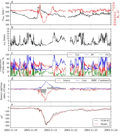
Figure 6. As figure 4, but for the storm beginning 20 November 2003.
8. Case studies
Figures 4, 5, and 6 show the results of NARMAX model run 1A during three geomagnetic storms,
re-connection, and the purely exponential decay term of equation 6a. A breakdown of the percentage losses from each of these processes is given in panel c.
Panel d compares the magnitude of the source term with the combined loss term. The source is the merg-ing of magnetic field on the dayside −a∆Φd (equation 6c), and has units of nT per minute. The shaded re-gion shows the overall rate of change of SYM-H∗, ie the combination of source and loss, also in nT per minute. Panel e shows the measured value of SYM-H (black), and the model values (red). The model results are cal-culated iteratively using the NARMAX model terms to calculate the next value of SYM-H based on the pre-vious model value, and solar wind data. The iteration begins at least 4 hours prior to the time period of in-terest, to allow it to converge and become independent of the starting value.
[image:13.595.71.303.647.760.2]Each of the three events show a similar picture. At storm commencement, rapid increases in solar wind ve-locity and negative BZ, are followed by an increase in the source term (−a∆Φd), with a 20 to 30 minute lag. The losses of SYM-H increase much more slowly. Ini-tially, and while the storm is being driven by the solar wind, the losses are mostly incurred in the tail recon-nection (see panel c). During this time a large pro-portion of the SYM-H value comes from the distorted magnetotail. As the open magnetic field in the tail re-connects, most of the energy is lost to Joule heating, particle precipitation, and the plasmoid, and therefore the magnetotail contribution to SYM-H is not wholly replaced by the increase in ring current. In the de-clining phases of the storms the losses are mostly due to the idealized loss term, (equation 6a,) which is as-sumed to primarily represent charge exchange (particle precipitation) losses. These features, and the overall loss rate, match those given by the of the numerical model of Kozyra and Liemohn [2003]. It is clear from figure 5 panel d that the NARMAX model is capable of reproducing the smallest of changes seen in SYM-H, but the longer term decay following the storm is not as accurate. While the model makes good use of high reso-lution solar wind data, it lacks the complicated physics and wave-particle interactions that control acceleration and loss inside the magnetosphere.
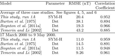
Table 6. A performance comparison of SYM-H and Dst
models.
Model Parameter RMSE (nT) Correlation
Coefficient Average of three case studies. See figures 4, 5, and 6
This study, run 1A SYM-H 20.4 0.952
Burton et al.[1975] Dst 38.1 0.894
Boynton et al.[2011a] Dst 19.3 0.966 Temerin and Li[2002] Dst 43.2 0.885 17 March 2000 to 9 May 2000.
This study, run 1A SYM-H 11.0 0.959
Burton et al.[1975] Dst 14.5 0.891
Boynton et al.[2011a] Dst 11.5 0.948 Temerin and Li[2002] Dst 9.26 0.961
9. Performance of the model
The aim of this study is to quantify the individual physical processes involved in solar-wind – magneto-sphere coupling, and identify their time lags, rather than produce a model for SYM-H. However, in this sec-tion we look at the performance of the model (run 1A) in reproducing SYM-H. For the three case studies in the previous section, the average RMSE of the model derived SYM-H is 20.4 nT, and the correlation coeffi-cient is 0.952. For comparison, we have implemented the models of Temerin and Li [2002], Boynton et al.
[2011a], andBurton et al.[1975], and provide the RMSE and correlation coefficients for each of the models in ta-ble 6. The models are also tested over the period 17 March 2000 to 9 May 2000. This time span is chosen because it has been excluded from the data used to pro-duce all four of the models. AlthoughTemerin and Li
[2006] provides an updated version of theTemerin and Li[2002] model, it is not used here because it is trained on the data from this test period, giving it an unfair advantage. The present model compares favorably with the others, although it may be at a disadvantage due to the high time resolution of SYM-H, which could natu-rally lead to higher RMSE than the low resolution Dst index. The model of Temerin and Li [2002] is by far the most complicated of the four models. It performs very well overall, but poorly for the large storm of the third case study (20 November 2003).
10. Summary
There are some limitations in the method and re-sults of the models presented in this study. Firstly, the NARMAX algorithm can only select from finite set of candidate predictors. Some coupling processes might not be well represented by any of the available choices. This is likely the case with the model flowout terms. The actual flowout rate depends on multiple different lags of solar wind parameters, these determine the den-sity of ring current particles, and control the dayside loss rate of those particles by altering the location of the magnetopause. Secondly, the maximum lag time in the models is 4 hours. Some magnetospheric processes take longer than this. For example, high energy (MeV) particles respond with 5 to 40 hour delays to solar wind enhancements [Li et al., 2005]. These particles are ener-gized in different processes to the lower energy particles that dominate the ring current. However, their popula-tions are too small to significantly affect SYM-H.
magne-totail reconnection is 60 to 120 minutes. These times match the impulse response of the AL index to changes in solar windvBS, which is observed to have two peaks at 20 min and 60 min [Bargatze et al., 1985]. Note that although tail reconnection causes a decay in -SYM-H, this is not the case with the AL index, which responds positively to substorm expansion.
It is difficult to say which of the model runs will pro-vide the truest representation of any particular geomag-netic storm. There are slight variations in the perfor-mance of the models depending on the particular event. The most significant difference between the models is the division of losses between the different loss mech-anisms. Any of the models that include the flowout loss term (ie models 1A, 1B, 2A, 4A, 4B, or 5A) should be equally valid, within the errors of this investigation. We would recommend using model 1A, for ease of com-parison with the results of this study, and because it provides values of SYM-H slightly closer to the mea-surements during the largest storms.
The models provide empirical evidence for the theory ofVasyli¯unas[2006], namely that the negative swings in Dst and SYM-H, which are described by the well known coupling functions, are firstly an observation of the open geomagnetic field piling up in the magnetotail and en-hancing cross-tail currents. When particles are injected on the nightside during tail reconnection, -SYM-H de-cays. This is because the loss of -SYM-H from the dipo-larization of the geomagnetic tail is greater than the gain in -SYM-H from the particle injection. Although
Vasyli¯unas [2006] expected the effects of dipolarization and injection to almost cancel, this result is in agree-ment with other studies [Iyemori and Rao, 1996;Siscoe and Petschek, 1997].
Acknowledgments. This work was supported by the
Natu-ral Environmental Research Council grant NE/J007773/1. The OMNI data are available from the GSFC/SPDF OMNIWeb in-terface at http://omniweb.gsfc.nasa.gov. SYM-H data is avail-able from the World Data Center for Geomagnetism, Kyoto, at http://wdc.kugi.kyoto-u.ac.jp/.
References
Bargatze, L. F., D. N. Baker, R. L. McPherron, and E. W. Hones (1985), Magnetospheric Impulse Response for Many Levels of Geomagnetic Activity,J. Geophys. Res.,90, A7, 6387–6394. Billings, S. A., and H. L. Wei (2005), he wavelet narmax
rep-resentation: A hybrid model structure combining polynomial models with multiresolution wavelet decompositions, Int. J. Systems Science,36, 137–152.
Billings, S. A. (2013), Nonlinear System Identification: NAR-MAX Methods in the Time, Frequency, and Spatio-Temporal Domains, John Wiley & Sons, ISBN 978-1-119-94359-4. Boynton, R. J., M. A. Balikhin, S. A. Billings, A. S. Sharma, and
O. A. Amariutei (2011), Data derived NARMAX Dst model, Ann. Geophysicae,29, 965 – 971, doi:10.5194/angeo-29-965-2011.
Boynton, R. J., M. A. Balikhin, S. A. Billings, H. L. Wei, and N. Ganushkina (2011), Using the NARMAX OLS-ERR algo-rithm to obtain the most influential coupling functions that affect the evolution of the magnetosphere, J. Geophys. Res., 116, A05218, doi:10.1029/2010JA015505.
Burton, R. K., R. L. McPherron, and C. T. Russell (1975), An empirical relationship between interplanetary conditions and Dst,J. Geophys. Res.,80, 4204–4214.
Dessler, A. J., and E. N. Parker (1959), Hydromagnetic theory of magnetic storms,J. Geophys. Res.,64, 2239–2259.
Dusik, S., G. Granko, J. Safrankova, Z. Nemecek, and K. Je-linek (2010), IMF cone angle control of the magnetopause location: Statistical study, Geophys. Res. Lett., 37, L19103, doi:10.1029/2010GL044965.
Hoffmann, W. (1989), Iterative algorithms for Gram-Schmidt or-thogonalization,Computing,41(4), 335–348.
Hong, X. and C. J. Harris (2001), Nonlinear model selection struc-ture detection using optimum experimental design and orthog-onal least squares,IEEE Transactions on Neural Networks 12 (2), 435–439.
Ieda, A., S. Machida, T. Mukai, Y. Saito, T. Yamamoto, A. Nishida, T. Terasawa, and S. Kokubun (1998), Statistical anal-ysis of the plasmoid evolution with Geotail observations J. Geophys. Res.,103, A3, 4453–4465.
Iyemori, T., and D. R. K. Rao (1996), Decay of the Dst field of geomagnetic disturbance after substorm onset and its implica-tion to storm – substorm relaimplica-tion,Ann. Geophysicae,14, 608 – 618.
Kamide, Y., and W. Baumjohann (1993), Magnetosphere-Ionosphere Coupling, Springer-Verlag, New York, ISBN: 978-3-642-50064-0.
Kan, J. R., and L. C. Lee (1979), Enery coupling and the solar wind dynamo,Geophys. Res. Lett.,6, 577.
King, J. H., and N. E. Papitashvili (2006), Solar wind spatial scales in and comparisons of hourly Wind and ACE plasma and magnetic field data, J. Geophys. Res., 110, A02104, doi:10.1029/2004JA010649.
Kozyra, J. U., and M. W. Liemohn (2003), Ring current energy input and decay,Space Sci. Reviews.,109, 105–131.
Lopez, R. E., W. D. Gonzalez, V. Vasyli¯unas, I. G. Richardson, C. Cid, E. Echer, G. D. Reeves, P. C. Brandt (2015), Decrease in SYM-H during a storm main phase without evidence of a ring current injection, J. Atmos. Sol.-Terr. Phys.,134, 118–129, doi:10.1016/j.jastp.2015.09.016
McPherron, R. L., and T. P. O’Brien (2001), Predicting geo-magnetic activity: The Dst index,Space Weather, Geophys. Monogr. Ser.,125, edited by P. Song, H. Singer, and G. Siscoe, 339–345.
Sckopke, N. (1966), A general relation between the energy of trapped particles and the disturbance field near Earth,J. Geo-phys. Res.,71, 3125.
Scurry, L., and C. T. Russell (1991), Proxy studies of energy transfer to the magnetopause,J. Geophys. Res.,96, 9541. Siscoe, G. L. (1970), A Virial Theorem Applied to
Magneto-spheric Dynamics,J. Geophys. Res.,75, 28, 5340–5350. Siscoe, G. L., and H. E. Petschek (1997), On storm weakening
during substorm expansion phase,Ann. Geophysicae,15, 211– 216.
Tanskanen, E. I. (2002), Terrestrial substorms as a part of global energy flow,FMI Contributions (36), ISBN 952-10-0423-1. Temerin, M., and X. Li (2002), A new model for the prediction
of Dst on the basis of the solar wind,J. Geophys. Res.,107, A12, 1472, doi:10.1029/2001JA007532.
Temerin, M., and X. Li (2006), Dst model for 1995 – 2002, J. Geophys. Res.,111, A04221, doi:10.1029/2005JA011257. Vasyli¯unas, V. M. (2006), Reinterpreting the
Burton-McPherron-Russell equation for predicting Dst, J. Geophys. Res., 111, A07S04, doi:10.1029/2005JA011440.
Vasyli¯unas, V. M. (2006), Ionospheric and boundary contribu-tions to the Dessler-Parker-Sckopke formula for Dst,Ann. Geo-physicae,24(3), doi:10.5194/angeo-24-1085-2006.
Wang, C., J. P. Han, H. Li, Z. Peng, and J. D. Richardson (2014), Solar wind-magnetosphere energy coupling function fitting: Results from a global MHD simulationJ. Geophys. Res. Space Physics,119, 6199–6212, doi:10.1002/2014JA019834. Wanliss, J. A. and K. M. Showalter (2006), High-resolution
global storm index: Dst versus SYM-H,J. Geophys. Res.,111, A02202, doi:10.1029/2005JA011034.
Wygant, J. R., R. B. Torbert, and F. S. Mozer (1983), Compar-ison of S3-3 polar cap potential drops with the interplanetary magnetic field and models of magnetic reconnection,J. Geo-phys. Res.,88, 5727.