Metastability in a condensing zero range process in the thermodynamic limit

Original citation:

Armendáriz, Inés, Grosskinsky, Stefan and Loulakis, Michail. (2016) Metastability in a

condensing zero-range process in the thermodynamic limit. Probability Theory and

Related Fields (In Press)

Permanent WRAP URL:

http://wrap.warwick.ac.uk/81696

Copyright and reuse:

The Warwick Research Archive Portal (WRAP) makes this work by researchers of

the University of Warwick available open access under the following conditions.

Copyright © and all moral rights to the version of the paper presented here belong to

the individual author(s) and/or other copyright owners. To the extent reasonable and

practicable the material made available in WRAP has been checked for eligibility

before being made available.

Copies of full items can be used for personal research or study, educational, or

not-for profit purposes without prior permission or charge. Provided that the authors, title

and full bibliographic details are credited, a hyperlink and/or URL is given for the

original metadata page and the content is not changed in any way.

Publisher’s statement:

The final publication is available at Springer via

http://dx.doi.org/10.1007/s00440-016-0728-y

.

A note on versions:

The version presented here may differ from the published version or, version of

record, if you wish to cite this item you are advised to consult the publisher’s version.

Please see the ‘permanent WRAP URL’ above for details on accessing the published

version and note that access may require a subscription.

Metastability in a condensing zero-range process in the

thermodynamic limit

In´es Armend´ariz

, Stefan Grosskinsky

, Michail Loulakis

June 15, 2016

Abstract

Zero-range processes with decreasing jump rates are known to exhibit condensation, where a finite fraction of all particles concentrates on a single lattice site when the total density exceeds a critical value. We study such a process on a one-dimensional lattice with periodic boundary conditions in the thermodynamic limit with fixed, super-critical particle density. We show that the process exhibits metastability with respect to the condensate location, i.e. the suitably accelerated process of the rescaled location converges to a limiting Markov process on the unit torus. This process has stationary, independent increments and the rates are characterized by the scaling limit of capacities of a single random walker on the lattice. Our result extends previous work for fixed lattices and diverging density in [J. Beltran, C. Landim, Probab. Theory Related Fields,152(3-4):781-807, 2012], and we follow the martingale approach developed there and in subsequent publications. Besides additional technical difficulties in estimating error bounds for transition rates, the thermodynamic limit requires new estimates for equilibration towards a suitably defined distribution in metastable wells, corresponding to a typical set of configurations with a particular condensate location. The total exit rates from individual wells turn out to diverge in the limit, which requires an intermediate regularization step using the symmetries of the process and the regularity of the limit generator. Another important novel contribution is a coupling construction to provide a uniform bound on the exit rates from metastable wells, which is of a general nature and can be adapted to other models.

AMS 2010 Mathematics Subject Classification: 60K35, 82C22; 60J45, 82C26, 60J75

Keywords: Metastability, Zero Range Process, Condensation.

∗_{Departamento de Matem´atica, Universidad de Buenos Aires, C1428EGA Buenos Aires, Argentina.}

Email:[email protected]

†_{Mathematics Institute, Zeeman Building, University of Warwick, Coventry CV4 7AL, UK.}

Email:[email protected]

‡_{School of Applied Mathematical and Physical Sciences, National Technical University of Athens, 15780 Athens, Greece.}

Contents

1 Introduction 3

2 Notation and main result 5

2.1 Notation . . . 5

2.2 The trace process and main result . . . 6

3 Proof of the main result 8

3.1 Proof of Theorem 2.2 . . . 8

3.2 Discussion . . . 11

4 Equilibration dynamics in the wells 14

4.1 Proof of Proposition 3.3 . . . 14

4.2 Proof of Lemma 4.1 . . . 16

5 Uniform bounds on exit rates via coupling 22

5.1 Construction of the coupling . . . 22

5.2 Proof of Lemma 3.5 . . . 24

5.3 Proof of Proposition 2.1 – Replacement by the trace process . . . 29

6 Regularization and inter wells dynamics 30

6.1 Rate estimates from capacity bounds . . . 31

6.2 Proof of Proposition 3.4 . . . 32

7 Capacity estimates 35

7.1 Lower bound . . . 35

7.2 Upper bound . . . 38

8 Tightness and Limiting Distribution 47

8.1 Proof of Proposition 3.1 – Tightness . . . 47

8.2 Proof of Proposition 3.2 – Martingale convergence . . . 49

8.3 Uniqueness for the martingale problem . . . 50

1

Introduction

A rigorous understanding of metastability phenomena in stochastic particle or spin systems has been a subject of major recent research. Intuitively, in such systems, the configuration space contains two or more disjoint metastable sets (called wells in the following) with an associated separation of time scales phenomenon in the scaling limit of a system parameter. In each well, the process spends a very long time which allows it to equilibrate to a metastable state. Exits from wells are then triggered by rare fluctuations, which lead to exponentially distributed waiting times in a well. Once activated, transitions to other wells occur on a much faster time scale, and do not depend on the detailed past of the sample path. So the limiting metastable dynamics corresponds to an effective Markov process on a highly reduced state space of metastable states associated to the wells. On a mathematically rigorous level, important conceptual questions of current research interest include a proper definition of metastable states in terms of probability measures, as well as a general practical framework to establish the separation of time scales. An important aspect in this context is the precise definition of metastable wells and in particular an optimal choice of their size, which is to some extent arbitrary. Intuitively, maximizing the depth and minimizing the complexity, or size, of the wells leads to a stronger separation of time scales. In combination they effectively characterize the free energy landscape for the chosen definition of wells in analogy to the classical framework of competition between energy (depth) and entropy (complexity).

Different approaches to metastability are summarized in [40], Chapter 4, including a pathwise treatment [20] which is based on an analysis of empirical averages along typical trajectories, and has more recently been studied also in [28]. For reversible systems a powerful potential theoretic approach has been developed [17, 18], using systematically the concept of capacities to establish sharp estimates on expected transition times between metastable states. This technique was applied in various models and is summarized in the new monograph [15] and the review papers [14, 22]. Potential theoretic methods have been applied to a particular family of condensing zero-range processes in [7, 6], leading to the development of a martingale approach summarized in [9] which we follow in this paper. Instead of deriving exponential limit distributions of individual exit rates from metastable wells directly, the limit process is identified as a Markov process via the solution to a martingale problem.

The zero-range process was introduced in [44] as a stochastic particle system without restriction on the local occupation numbers, where the jump rates of particles depend only on the occupation number of the departure site. The dynamics locally conserves the number of particles and the process is known to have a family of stationary product measures [1], which can be indexed by the particle densityρ. Under certain conditions on the jump rates this family has a maximal element at a finite (critical) densityρc, and the process exhibits a condensation transition. Conditioned on densitiesρ > ρc the system phase separates into a homogeneous phase distributed at the critical product measure, and a condensate, where the remaining mass concentrates in a single lattice site for typical stationary configurations of large, finite systems. This phenomenon was first reported in the theoretical physics literature [25, 27], and rigorous results including the equivalence of ensembles, a law of large numbers and a central limit theorem for the condensate size have been established in [36, 35, 3]. In spatially inhomogeneous zero-range processes a condensation phenomenon can occur that has different dynamic and static features as discussed above, and can be studied with the help of coupling techniques (see e.g. [4] and references therein). In this paper we focus on spatially homogeneous systems, which are necessarily non-monotone [41] and where basic coupling techniques cannot be applied.

in [7, 6] in a slightly more general setting allowing for spatial inhomogeneities, but these results are restricted to a fixed lattice in the limit of diverging particle numberN. In this setting, the depth of metastable wells dominates their complexity and they are relatively small sets. Repeated visits to particular configurations occur before the process exits the well (often called attractor states), which provides a renewal structure that can be used to establish the separation of time scales. The limit process of the condensate location is then a continuous-time random walk on the fixed lattice, where transition rates are proportional to the capacities of a single random walker. For the same model, matching upper and lower bounds for exit rates from metastable wells have been derived in [19] in the limitL, N → ∞

with diverging particle densityN/L→ ∞(see also [15], Chapter 21).

In this paper we establish the full metastable limit dynamics for the condensate location for the above family of reversible zero-range processes in the thermodynamic limit, i.e. we takeL, N → ∞

with finite, supercritical density N/L → ρ > ρc. We consider a one-dimensional system with periodic boundary conditions, which leads to a L´evy-type limit process for the rescaled condensate location on the unit torus with stationary, independent increments. A major new difficulty is related to thermalization within the metastable wells, which are exponentially large in the system size and previously applied renewal techniques do not apply. To separate the slow and fast variables effectively, we describe the thermalization dynamics on the wells using the restricted process introduced in [12] and [9]. We can then prove relaxation time bounds for this process by a comparison argument with independent birth-death chains. Another key ingredient is a uniform bound on exit rates from a well which is established by a novel coupling construction and is used in several occasions in our proof, including thermalization. The characterization of the limiting generator of the process is more difficult in the thermodynamic limit due to increasing complexity of the free energy landscape, caused by the diverging number of wells and transition paths between them. To tackle this we have to introduce an intermediate regularization step on a coarse-grained lattice using the full symmetries of the model and regularity of the limit process. We note that, similarly to the results in [19] for diverging particle density, we are not able to establish matching bounds for transition rates between individual wells. But in order to identify the limit process it is sufficient to get matching bounds only between regularized sets of wells. As in previous results on this model, the leading order of transition rates between wells is polynomial in the system sizeL, which requires sharp estimates on transition rates from potential theory. Due to the increasing complexity of transition paths we need a better control than results in [7, 6] on the leading order error terms, which constitutes an additional technical difficulty. We note that a rescaling argument in a different context has also been used in [38] to establish metastability for the ABC model.

So far, there are only few metastability results that deal with infinite volume limits as summarized in [15], Part VII. Examples include kinetic Ising models at low temperatures [16] or low magnetic fields [43], results on the dynamics of critical droplets [33], or dilute gases at vanishing density and temperature [30]. All these results feature the additional scaling of a system parameter such as temperature or density, which increases the depth of metastable wells compared to their complexity. Often this is a necessary requirement for metastability to occur at all, and in [19] this has been used as a simplifying assumption to obtain results for the zero-range process in an infinite density limit. To our knowledge, the thermodynamic limit result derived here without any scaling of system parameters constitutes therefore one of the first metastability results of this kind.

given in Section 7, and Sections 8 and 9 contain auxiliary results on tightness, martingale convergence and properties of the stationary measure.

2

Notation and main result

2.1

Notation

Consider the zero-range process η(t) :t≥0on the one-dimensional discrete torusΛ =Z/LZwith

Nparticles and state space

XL,N =

η∈NΛ0 :SL(η) =N where we denote SL(η) = X

x∈Λ

ηx. (2.1)

The dynamics is defined by the generator

Lf(η) = X

x,y∈Λ

p(x, y)g(ηx) f(ηx,y)−f(η)

(2.2)

for all continuous functionsf :XL,N → R, with the usual notationηzx,y =ηz−δz,x+δz,y,z ∈ Λ for the configurationηx,y _{where one particle has moved from sitexto sitey. We focus on symmetric,} nearest neighbour jump probabilitiesp(x, y) = 1₂δy,x−1+1₂δy,x+1with periodic boundary conditions, and jump rates are of the form

g(0) = 0, g(1) = 1 and g(n) = n

n−1

b

forn≥2, with parameterb >0. (2.3)

Without the canonical constraintSL=N, the process is known to exhibit a family of stationary product measures with a maximal elementν[1, 27, 36, 35], which has marginals

ν[ηx=n] =

1

zc

1

g!(n) with g!(n) =

n Y

k=1

g(k) =nb forn≥1 and g!(0) = 1. (2.4)

As long asb >2the normalization and first moment ofνare both finite, i.e.

zc:= 1 +

∞

X

n=1

n−b<∞ and ρc:=ν(ηx) =

1

zc

∞

X

n=1

n1−b <∞. (2.5)

The process is irreducible onXL,N and the corresponding unique stationary measuresµL,N are called canonical distributions, and can be written as conditional product measures

µL,N =ν ·

SL=N. (2.6)

To simplify notation we will writeµ=µL,N from Section 3 onwards.

We study the large scale behaviour of the process in the thermodynamic limit with particle density ρ≥0, i.e.

L, N=NL→ ∞, such thatN/L→ρ . (2.7)

Forb >2andρ > ρc(2.5), the process is known to exhibit a condensation transition in the following sense. Denoting by

ML= max

the maximum occupation number as a relevant order parameter, we have a weak law of large numbers [27, 36, 35]

ML/L→

0 , ρ≤ρc

ρ−ρc, ρ > ρc

asL, N → ∞(2.7), (2.9)

where convergence holds in distribution w.r.t. the sequenceµL,N. A corresponding CLT has been es-tablished in [3], and the fluctuations are Gaussian and of order√Lforb > 3, and of orderL1/(b−1) with an associated stable law for2< b≤3. Moreover, the distribution of the configuration outside the maximum is known to converge to the maximal product measureν with densityρcin the limit (2.7), so the largest occupation number in the bulk outside the maximum is typically of orderL1/(b−1)L, which holds for allb >2independently of the fluctuations of the maximum. Therefore for supercritical densitiesρ > ρcconfigurations exhibit a unique extensive maximum with high probability, called the condensate, and the rescaled location of the maximum

ψL(η) =

1

L

x∈Λ :ηx=ML(η) (2.10)

is given by a single site in the rescaled lattice_L1Λ. By translation invariance,ψLis distributed uniformly in_L1ΛunderµL,N, and ergodicity of the process onXL,N implies thatψL η(t)visits the whole lattice on a long time scale. It is expected that this dynamics is metastable, i.e.ψL η(t)

is constant for a long (random) time interval, and then changes abruptly to a new value which depends only on the current location of the condensate.

Our main result is that, indeed, for large enoughb > 2andρ > ρcthe zero-range process η(t) :

t≥0in the thermodynamic limit (2.7) exhibits metastability with respect to the observableψLon the time scale

θL:=L1+b. (2.11)

This means that the sequence of processes _L1 ψL(ηtθL) :t≥0

converges to a Markovian limit process on the unit torus_T = _R/_Z, the scaling limit of _L1Λ. A rigorous version of this result is provided in the next subsection in Theorem 2.2, including an exact formulation of the mode of convergence and required assumptions.

2.2

The trace process and main result

The rigorous formulation and proof of our main result on the large scale metastable dynamics of the condensate follows the martingale approach developed in [7, 6, 9], which requires a partition of the state space as a first step. We define the wellEx_{as the set of configurations where the condensate is located} atx∈Λ,

Ex_:=

η ∈XL,N :ηx=ML≥N−ρcL−αL, ηy≤βLfor ally6=x . (2.12) We choose the scales in this definition as

αL =L 1

2+25b _{and βL= 2}b_L

4

b−1c_{, (2.13)}

which allow for typical fluctuations of the condensate size of order√L, and of bulk occupation numbers of orderL1/(b−1) _{for anyb > 3. Note that under our conditions onbin Theorem 2.2 we also have} αL, βL L. We chooseβLas a sequence of integers for later convenience, while the exponent inαL is optimal for the estimates in Section 6.2. We denote by

the set of all wells and its complement. The first result states that the process started from a well spends only a negligible amount of time on the set∆ on the timescaleθL. As usual, we denote by Pη and

Eη the path measure and expectation of the processη(·)with generator (2.2) and with initial condition

η(0) =η.

Proposition 2.1 Replacement by the trace process

For the process defined in (2.2) with rates (2.3) andb >20, we have for allt >0

sup

η∈EEη

hZ θLt

0

1∆(η(s))dsi.θL→0 asL, N→ ∞(2.7)withρ > ρc. (2.15)

The proof of this result is given in Section 5.3. The larger lower bound on the parameterb is a purely technical restriction which we discuss in Section 3.2. Since the process spends only negligible time outsideE, re-parametrizing time by the local time onEwill not change the process in the limit. Denote by

Tt:= Z t

0

1E(ηs)ds and St:= sup

s≥0 :Ts≤t (2.16)

the local time onEand its generalized inverse, respectively. The trace process is then defined as

ηE(t) :t≥0

with ηE(t) :=ηSt , (2.17)

which takes values in the setE and is well defined since Tt diverges Pη −a.s. as t → ∞due to the irreducibility on the finite state spaceXL,N. As is shown in [6], Section 6.1, (2.17) is in fact an irreducible Markov process onEwith jump rates

rE(η, ξ) :=r(η, ξ) +X

ζ∈∆

r(η, ζ)Pζ[TE =Tξ]. (2.18)

Herer(η, ξ) :=P

x∈Λg(ηx)1₂ 1ξ(ηx,x+1) +1ξ(ηx,x−1)

are the jump rates of the processη(·)with generator (2.2), and

TF:= inft≥0 :ηt∈ F (2.19)

denotes the hitting time of a setF ⊂XL,N. For point subsetsF ={ξ}we use the shorthandT{ξ}=Tξ. The trace process has generator

LEf(η) =X

ξ∈E

rE(η, ξ)f(ξ)−f(η), (2.20)

and reversible invariant measureµL,N

· E

restricted toE. To simplify notation, we will call

µE[·] =µL,N

· E

. (2.21)

On the set of wellsEthe rescaled location of the maximum can be written as

ψL(η) :=

1

L

X

x∈Λ

x1Ex(η)∈_T=_R/_Z, (2.22)

Theorem 2.2 Consider the zero-range process with generator (2.2) and rates (2.3) withb > 20. Fix a sequence of initial conditionsη(0)∈ E such thatψL(η(0))→Y0 ∈T. In the thermodynamic limit

(2.7) withN/L→ρ > ρcwe have for the trace process (2.17) on the time scaleθL=L1+b

ψL ηE(tθL)

:t≥0⇒ Yt:t≥0

, (2.23)

where convergence holds weakly on the path spaceD [0,∞),Tin the usual Skorohod topology.

The process(Yt : t ≥ 0) has stationary and independent increments onT, initial conditionY0 and

generator

LT_{f(u) =} Z

T\{0}

rT_{(v) f(u+v)−f(u)}

dv (2.24)

for all Lipschitz continuous functionsf :T→R, with rates

rT_{(v) =} 1

zcIb(ρ−ρc)b+1

1

d_T(0, v), v∈T. (2.25)

Embedding the unit torus in[0,1)⊂_R, the distance onTis given bydT(0, v) =|v|(1− |v|).zcis the

normalization of the invariant measure (2.5), and

Ib := Z 1

0

xb(1−x)bdx= Γ(b+ 1)

2

Γ(2b+ 2) (2.26)

is a constant depending only onb.

Note that (2.15) and our main result do not apply for initial conditions η(0) ∈ ∆, which are, however, untypical if the process starts from the stationary measureµL,N (cf. Corollary 9.5). The mode of convergence in terms of the trace process as presented here has been introduced in [7, 6], and extended recently in [9] to a more general context. The (random) time change in the definition of the trace process, which is negligible in the limitL→ ∞, can also be absorbed in a definition of a suitable topology on the path space of the limiting process. Further discussion, including possible extensions of our result, is provided in Section 3.2.

3

Proof of the main result

The proof of Theorem 2.2 uses a standard approach to establish existence of a limit process by a tightness argument, and to identify the limit by the solution of a martingale problem. We follow the method outlined in [9], proofs of auxiliary results used below are given in the rest of the paper. We also discuss the main novelties and possible extensions.

Here and in the following sections we adopt a few shorthands and conventions to avoid an overload of notation. We writeµ=µL,N for the invariant measure of the full process, andµE for the invariant measure of the trace process (2.21). Constants denoted byCare independent ofLandN, and can vary from line to line.

3.1

Proof of Theorem 2.2

The proof of convergence holds on arbitrarily large compact time intervals for the limit process, and throughout this section we denote the length of this interval byT >0. Let

be the speeded up process of the rescaled maximum location, and letQL be its distribution on path

spaceD [0, T],_T

.

Proposition 3.1 Tightness

Under the conditions of Theorem 2.2 withb > 20the sequenceQLof path space distributions is tight

onD [0, T],T.

The proof is given in Section 8 where a control of the quadratic variation excludes the accumulation of jumps and ensures that limit points have right-continuous paths. Tightness implies existence of sub-sequential weak limits ofQLin the Skorohod topology, and we denote any such weak limit byQ. In

order to identify the limit we need to show that for allt ≤ T and all Lipschitz-continuous functions f ∈Lip(T)

f(ωt)−f(ω0)−

Z t

0

LT_f(ω

s)ds is a martingale, (3.2)

whereωt: D [0,∞),T→ Tis the coordinate process on path space. Together with the uniqueness

result for the martingale problem associated withLT_{proved in Subsection 8.3, this implies convergence} ofQLand characterizes the limitQas the law of the Markov process Yt :t∈ [0, T]

with generator

LT _{(2.24), because Lipschitz functions form a core for this generator. SinceT > 0is arbitrary, this} implies Theorem 2.2. Precisely, we need to show that

EQ

g (ωu: 0≤u≤s)

f(ωt)−f(ωs)− Z t

s LT_f(ω

u)du

= 0, (3.3)

for all0≤s < t≤T and all bounded, continuous functionsg:D [0, T],_T

→_R. Since ηE(θLt) :

t∈[0, T]is a Markov process with generatorθLLE, we know that

f(Y_tL)−f(Y₀L)−θL Z t

0

LE(f◦ψL)(ηE(θLs))ds=

=f(Y_tL)−f(Y₀L)− Z t

0

LT_f(YL s )ds+

Z t

0

LT_f(YL

s )−θLLE(f◦ψL)(ηE(θLs))

ds

is a martingale for allt∈[0, T]andL∈_N. We will establish below that

sup

η∈EE

η

Z t

0

LT_f(YL

s )−θLLE(f◦ψL)(ηE(θLs))

ds

→0 (3.4)

asL→ ∞, which implies that

EQ

L

g (ωu: 0≤u≤s)

f(ωt)−f(ωs)− Z t

s LT_f(ω

u)du

→0, (3.5)

for all0 ≤s < t ≤ T and bounded, continuousg : D [0, T],T → R. To identify the limit of the

left-hand side with (3.3) we use the following result, which is immediate from Lemma 8.2 in Section 8.2.

Proposition 3.2 LetM_tf(ω) =f(ωt)−f(ωs)−R t

sLTf(ωu)du. Then

EQ

Lh

g (ωu: 0≤u≤s)

M_tf(ω)i→_EQh_{g (ω}

u: 0≤u≤s)

M_tf(ω)i (3.6)

To conclude the proof we have to show (3.4), i.e. that we can replace the generator of the trace process with that of the limit process (cf. Section 3 in [9]). This is the main part of the paper and is divided into several steps. Since we cannot compare the generatorsLE _andLT _{directly, we will} introduce an auxiliary processes on_Twith generatorLΛ _{which is explained in detail below, and we} rewrite the time integral in (3.4) as

Z t

0

LT_f(YL

s )−θLLE(f ◦ψL)(ηE(θLs))

ds=

=

Z t

0

LT_f(YL

s )−θLLΛf(YsL)

ds (3.7)

+θL Z t

0

LΛ_f(YL

s )− LE(f◦ψL)(ηE(θLs))

ds . (3.8)

The goal is now to show that the terms in (3.7) and (3.8) vanish individually asL → ∞inL1-norm. In (3.8) we compare the trace process to the auxiliary process on the rescaled lattice _L1Λ ⊂T, which

describes the effective jumps of the condensate location. Its generator is defined as

LΛ_{f(x/L) :=} X z∈Λ,z6=0

rΛ(z) f (x+z)/L−f(x/L), (3.9)

with jump rates (using translation invariance)

rΛ(z) = X

ξ∈Ez

µ|E0 rE(., ξ)

= 1

µ[E0_]

X

η∈E0

ξ∈Ez

µ[η]rE(η, ξ), (3.10)

given by the expected rate between wells for the trace process. Therefore, we can also write the generator (3.9) as the expectationLΛ_{f(x/L) =µ|}

Ex LE(f◦ψ_L). Before the location of the condensate changes, the process remains in the same wellEx_{for a long enough time to equilibrate, and the transition between} wells is effectively described by stationary averages of jump rates as in (3.10), which is established in the next result.

Proposition 3.3 Equilibration in the wells

Under the conditions of Theorem 2.2 withb >20,

sup

η∈EEη

θL Z t

0

LΛ_f(YL

s )− LE f ◦ψL

ηE(θLs)

ds

→0 (3.11)

asL→ ∞, for allt∈[0, T].

In addition to using Lemma 3.5 given below, the proof requires an estimate on the relaxation and mixing times within a well, which have to be strictly smaller thanθL, and is provided in Section 4.

In (3.7) we replace the generator of the auxiliary process with that of the limit process using the following result.

Proposition 3.4 Dynamics between wells

Under the conditions of Theorem 2.2 withb >5,

sup

η∈EE

η

Z t

0

LT_{f Y}L s

−θLLΛf YsL

ds

→0 (3.12)

The proof is given in Section 6 and requires sharp bounds on the transition rates of the auxiliary process, which are provided by capacity estimates in Section 7. In order to get matching upper and lower bounds, an important new step in this part of the proof is to regularize the ratesrΛ_{(z) on an} intermediate scale and use the regularity of the test functionf, which is explained in detail in Section 6. This finishes the proof of our main result, Theorem 2.2.

An important estimate that is used in the proof of tightness, equilibration and replacement of the trace process is the following uniform bound on the exit rate from a well. The proof of this Lemma is given by a coupling argument in Section 5, which is one of the crucial new results of this paper.

Lemma 3.5 Uniform bound on the exit rate

Under the conditions of Theorem 2.2 withb >20, there exists a constantC >0such that the exit rate from a well is uniformly bounded by

sup

η∈E0 X

ξ6∈E0

rE(η, ξ)≤ C

L5_log2_L . (3.13)

3.2

Discussion

Main new ideas. Our proof follows the martingale approach outlined in [9], which was previously applied to zero-range processes on a fixed lattice in the limitN → ∞[7]. In contrast to this case, the thermodynamic limit (2.7) considered here involves a significant change in the complexity of metastable wells, since the sizes of the wells and the number of transition paths between them increase withL. Following the discussion in [29], this presents a technically more challenging metastability scenario, in particular since the free energy barriers of the metastable wells in the zero-range process are only logarithmic. We quickly summarize the resulting conceptual and technical difficulties and the three main novel contributions of this paper to overcome them.

• In previous work with limits of diverging particle density [7, 19] the depth of the metastable wells was dominating their size, and they could effectively be replaced by individual configurations, so-called attractor states. The repeated visits to those configurations before hitting another well lead to a relatively simple renewal-type proof for equilibration in the wells. In our case of finite particle density the size of metastable wells increases exponentially withLand these types of arguments do not apply. Instead, we have to describe the metastable states as probability distribu-tions on wells. As outlined in [9, 29] a suitable candidate is simply the restriction of the stationary measure, and to prove Proposition 3.3 we use suitable dynamics restricted to a well following [9], see Section 4. Using a standard jacknife estimate [26] we establish a Poincar´e inequality compar-ing these dynamics to independent birth-death chains in Section 4.2, and obtain a bound on the relaxation time on the metastable well of orderL4in Lemma 4.1. This is clearly not optimal, and a sharp bound is expected to be of orderL2, which would moderately improve our conditions on the parameterbin Proposition 3.3 and Lemma 3.5, currentlyb >20, tob >13.

• Resulting from capacity bounds presented in Section 7, the transition rates between wellsrΛ(z)

address both issues in the standard thermodynamic limit for fixed density, using the symmetry of the system and the regularity of the limit dynamics on the unit torus, which are fully characterized by Lipschitz-continuous test functions. We regularize the dynamics on an intermediate scale in Section 6 to get matching bounds on rates between regularized sets of wells, which are sufficient to derive the limiting generator and prove Proposition 3.4. As an additional technical difficulty we have to keep track of corrections of capacity bounds to leading order in L, which require very precise estimates on the stationary measure summarized in Section 9. Sections 6 and 7 are independent of the rest of the proof, and the only restrictions on the parameterbarising there are given by equations (6.4) and (6.13), resulting in a much weaker condition ofb >5.

• While the limiting metastable dynamics are determined by stationary averages of transition rates rΛgiven in (3.10), a uniform control of the exit rates from a well is important to estimate error terms as is discussed in general in [9]. Some particular examples of spin systems where this has been achieved are mentioned in [15], but note that using capacities between individual configura-tions in the thermodynamic limit would lead to bounds that diverge exponentially in the system size. Here we derive a uniform upper bound on exit rates scaling asL−5_log−2_L

in Lemma 3.5, which is proved in Section 5 by a novel coupling construction with a growing number of birth-death chains. The number of chains increases only linearly in time, and the construction ensures that in the event of changing well, at least one of the chains has grown a condensate. This is a cen-tral auxiliary result of the paper, and is used in the proof of equilibration in the wells (Prop. 3.3), replacement by the trace process (Prop. 2.1), as well as for tightness (Prop. 3.1). The proof of Lemma 3.5 requiresb >20, and sharper estimates on equilibration times in wells would slightly improve this condition as mentioned above.

The bottleneck of the method leading to restrictive conditions on the parameterbresults from the inherent competition between depth and complexity of metastable wells. Both quantities increase with the size of the wells, and the aim to maximize depth and minimize complexity leads to an optimal choice of their size that enters most prominently in the uniform bounds on exit rates. The coupling argument in Section 5.1 gives a lower bound on the expected time to change wells for the full zero-range process. To turn this into an estimate for the trace process, we have to bound the time spent outside the wells on the set∆, which is controlled by the invariant measure in Corollary 9.5. Larger wells of increased depth improve this bound, but at the same time lead to an increase in the number of transition paths to other wells. Both effects compete and affect the uniform bound on the exit rates in Lemma 3.5. It turns out that the optimal size is controlled by the parameterβL(2.12), and the crucial estimate in this context is (5.24) for the probability that the trace process has changed well on the time scaleθL, where terms of the formβ_Lb−1 andβ_L1−b appear in bounds of the right-hand side. The best choice ofβLin (2.13) leads to a bound in Lemma 3.5 which is small enough for the required estimates in the proofs of Propositions 2.1, 3.1 and 3.3 as long asb >20. The mechanism leading to this constraint is of a funda-mental nature, and it seems very hard to significantly improve this with the techniques used in this paper.

Possible extensions. We focus on symmetric, nearest-neighbour probabilitiesp(x, y) = 1₂δy,x−1+ 1

2δy,x+1in one dimension with periodic boundary conditions, two properties of which are essential for our proof.

• Symmetry; this leads to reversible dynamics, which is a necessary condition for the potential the-oretic estimates on transition rates we use in Section 7. There is significant recent research interest on extended Dirichlet principles for non-reversible systems which involve double variational for-mulas [8, 10, 31], see also references in [15], Chapter 7. This has been applied to the totally asymmetric zero-range process on a fixed lattice in [37], but since a result in the thermodynamic limit requires much better control on error bounds an extenstion to this case would be a signif-icant technical complication. While a (non-optimal) relaxation time estimate for non-reversible systems can probably be obtained, we also make critical use of symmetry of the jump rates in the regularization step in Section 6, which is not obviously adapted to asymmetric situations.

• Translation invariance; the results in [7, 6] apply to zero-range processes without this property, leading to spatially inhomogeneous limit dynamics on a fixed lattice which are directly related to the choice ofp(x, y). We use translation invariance in our proof for equilibration and also in the regularization step in Sections 4 and 6. Specific simple examples of non-translation invariance, such as alternatingp(x, y)or isolated inhomogeneities, can be treated as a direct extension of our result on a case-by-case basis. However, it is not clear how to formulate a result in the generality covered in [7, 6], where the first problem already may arise when defining the limiting process if the probabilitiesp(x, y)do not have good scaling properties.

Whenever the p(x, y) are symmetric and translation invariant and admit a well defined scaling limit of the capacities of a single random walk onΛanalogously to (6.6), our results can be extended without much effort to lead to limit processes with stationary, independent increments. General finite range symmetric p(x, y) in one or higher dimensions which scale to Brownian motion should all give the same result related to the corresponding harmonic functions of a single walker, appropriately modified on the torus. Note that in three and more dimensions these functions have a constant scaling limit leading to uniform displacement of the condensate, with expected logarithmic corrections in two dimensions. Also ifp(x, y)has range diverging withLwith well defined scaling limits for capacities our result can be directly adapted, including for example uniform p(x, y) which leads to uniform condensate dynamics on the limiting torus. Due to the special properties of one-dimensional diffusion the case covered here is already one of the most interesting. Note also that even for finite-rangep(x, y)

the condensate dynamics will be non-local in all dimensions, in contrast to an analogous result for inclusion processes [34].

In addition to the jump ratesg(n)(2.3) considered here, there are various other choices that lead to condensing zero-range processes (see e.g. [41] and references therein). A well studied example is for rates with asymptotic behaviourg(n)∼1 +b/nλwithλ∈(0,1)leading to stretched exponential tails for the stationary measure [21, 2]. The lighter tail of the measure increases the depth of the metastable wells and leads to free energy barriers that grow sublinearly in the system sizeL, which is much faster than the logarithmic growth for the present model corresponding toλ = 1. There-fore, even though an actual generalization would require considerable work, we expect that all our techniques can be applied and some estimates, in particular the ones in Section 7, should even get easier.

The depth of metastable wells increases with particle density, and with the parameterbwhich deter-mines the tail of the stationary measure. In contrast to the restrictive conditions onb, our proof is robust in this system parameter and does not require any additional constraints on the particle density except ρ > ρc. As long as the excess massN−ρcL

√

interesting to investigate, but is beyond the scope of this paper, in how far our results can be applied also for subextensive excess mass.

Related work. The results presented here and other metastability results for zero-range processes only concern the stationary dynamics of a single condensate, corresponding to the slowest time scale in the system. In particular, these results only apply when the process is started on one of the metastable wells. Starting the process from a uniform initial condition with supercritical or diverging density leads to a dynamic formation of the single condensate on a different, faster time scale. This has been discussed heuristically in [35, 32], where it was found that after a rapid formation of several large clusters, they exchange particles in a coarsening process on the time scaleL3 L1+b which leads to the formation of a single condensate. Note that the location of the clusters on this time scale is fixed. Recently the first rigorous result in this context has been obtained on a fixed lattice in the limit N → ∞in [5]. The coarsening dynamics takes place outside the setE and is therefore approached with entirely different methods than the ones in this paper. For the condensation phenomenon in the inclusion process the dynamics of the condensate and the coarsening process take place on the same time scale, and both have been rigorously understood in [34].

4

Equilibration dynamics in the wells

To establish an upper bound for the thermalization time scale of the trace process in a metastable well we follow the procedure outlined in [9]. We introduce a process restricted to the well (called reflected process in [9]), which is reversible w.r.t. the restricted measureµ, and estimate the relaxation time of this process. A general result from [9] can then be applied to yield a simple proof of Proposition 3.3.

4.1

Proof of Proposition 3.3

For each wellEx_{,x∈Λ, the restricted process is defined by the generator}

Lx_{f(η) =} X ζ∈Ex

r(η, ζ) f(ζ)−f(η)

for allη∈ Ex_{. (4.1)}

As before,r(η, ζ)denote the jump rates of the full zero-range process, and jumps outside the wellEx are suppressed. Note that this is not equal to the trace process onEx_{, which has additional rates at the} boundary ofEx_{. It is easy to see that this process is irreducible onE}x_{and that it is reversible w.r.t. the} restricted measure

µx:=µ[.|Ex_{]. (4.2)}

The following estimate on the relaxation and mixing times of the restricted process will be used to prove Proposition 3.3.

Lemma 4.1 The relaxation timetreland the-mixing timetmix()of the restricted processLx(4.1) on

Ex_{are independent ofxand bounded by}

trel ≤CL4 and tmix()≤CL5(1 +L−1log1), (4.3)

The proof of this Lemma uses path counting techniques to establish a Poincar´e inequality for the re-stricted process, which is independent of the rest of this section and is therefore postponed to Subsection 4.2.

We will use the followingL2_{estimate for the ergodic average of a function that has mean zero on} all wells, starting from the stationary measureµE =µ[.|E]restricted to the wells. The proof of can be found in [9], Section 3.1.

Lemma 4.2 For every functionf :E →Rwhich has vanishing meanµx(f) = 0for allx∈Λ, and for

allt >0

EµE

Z t

0

f(ηE(s))ds

2

≤24tX

x∈Λ

µ[Ex]txrelµ

x

(f2), (4.4)

wheretx

rel =trelis the relaxation time onExof the restricted process, which does not depend onxin

our case.

By translation invariance we can simply focus on initial conditions in a chosen wellE0 _{in the} fol-lowing. To prove Proposition 3.3 we have to show (3.11), i.e. prove that

Eη

Z θLt

0

LΛ_{f ψ}

L(ηE(s))− LE f◦ψL ηE(s)

ds

=Eη

Z θLt

0

X

z∈Λ

z6=0

rΛ(z)−rE(η(s),Ez₎

f ψL(η(s)) +z/L−f ψL(η(s))

→0 (4.5)

asL → ∞for all Lipschitz functionsf : T → Randη ∈ E0. For the total jump rate of the trace

process into another wellz6= 0, we have used the obvious notation rE(η,Ez_{) =} X

ζ∈Ez

rE(η, ζ) for allη ∈ E0_.

With the definition ofrΛ_{(z)in (3.10) we have} rΛ(z) =µxrE(.,Ex+z₎

for allx, z∈Λ,

and since the functionf◦ψLis constant on all wells, the function

hf(η) := X

z6=0

rΛ(z)−rE(η,Ex+z)f ψL(η) +z/L

−f ψL(η)

(4.6)

has mean zero underµx_{for allx∈Λ, independently off. On every wellE}x_{, we can estimate its second} moment as

µx h2_f ≤µx

X

z6=0

rE(·,Ex+z_{)f ψ} L(·) +

z L

−f ψL(·)

2

≤C_f2µx

X

z6=0

rE(·,Ex+z₎2

≤Cf

X

z6=0

rE(·,Ez_{) ∞}

X

z6=0

rΛ(z)≤CCf

1

L5_log2_L

logL θL

, (4.7)

Here,Cf is the Lipschitz constant off. The last inequality follows from (3.13) in Lemma 3.5 and equation (6.7), derived independently from capacity estimates in Section 7. The latter implies that the espected total exit rate

θL X

z6=0

With Lemmas Lemma 4.2 and 4.1, this implies that

EµE

Z tθL

0

hf(η(s))ds 2

≤CCftθL

1

L5_log2_LL 4logL

θL

=CCft

1

LlogL, (4.9)

with initial condition under the stationary distributionµE. Now

sup

x∈ΛE

µx

Z tθL

0

hf(η(s))ds 2

≤X x∈Λ

Eµx

Z tθL

0

hf(η(s))ds 2

=LEµE

Z tθL

0

hf(η(s))ds 2

,

and therefore

sup

x∈ΛE

µx

Z tθL

0

hf(η(s))ds 2

≤CCft

1

logL. (4.10)

Finally, we use Lemma 3.5 and our estimate on the mixing time in Lemma 4.1 to get forof order1/θL

Eη

Z tθL

0

hf(η(s))ds

≤Eη

Z tmix()

0

hf(η(s))ds

+Eη

Z tθL

tmix()

hf(η(s))ds

≤Cf

X

z6=0

rE(·,Ez₎

∞ tmix() +tθL

+ sup

x∈Λ

Eµx

Z tθL

0

hf(η(s))ds

21/2

≤CCf

L5+t 1

L5_log2

L+

p

t/logL−→0 as L→ ∞. (4.11)

This finishes the proof of Proposition 3.3.

4.2

Proof of Lemma 4.1

We will derive an upper bound on the relaxation time of the restricted process in a well by proving a Poincar´e inequality, due to translation invariance it is enough to focus on the wellE0_{. We will use that} the stationary measureµ0_{outside the condensate location is essentially given by a product measure at} the critical density in the limitL→ ∞. Withµ[E0_{] =µ[E]/Lwe can write}

µ0[η] =µ0

(η0, ηΛ\0)

=νL−1[ηΛ\0] ν1_[η

0] νL_[S

L=N]

L

µ[E] , (4.12)

where we use the notationη = (η0, ηΛ\0)forη ∈ E0to indicate the condensate sizeη0 and the bulk configurationηΛ\0 outside the condensate. For fixed particle numberN (i.e. under the measureµ), ηΛ\0 obviously uniquely determines η0. To simplify notation we identify measures with their mass function, and to avoid possible confusion in this section we will indicate the dimension of the product measureνin each term with a superscript.

We interpret the product measureνL−1_{in (4.12) as the stationary measure of an auxiliary system} ofL−1independent birth death chains with birth rate 1and death rateg(n). Corresponding to our definition of the metastable wells in (2.12), we restrict the state space of the chains toX ={0, . . . , βL}. Each chain has therefore the modified stationary measure

¯

ν1=ν1[.|X] and ν¯1[n] = ν

1_[n]

ν1_[X] for alln∈X . (4.13)

Lemma 4.3 There exists aC >0such that for allf :XL−1_→

Rand allLlarge enough

Varµ0(f)≤CνL−1[XL−1]Var_ν¯L−1(f1_B0). (4.14)

Here

B0=nζ∈XL−1:N− L−1

X

x=1 ζx, ζ

∈ E0o₌n_ζ∈XL−1_:

L−1

X

x=1

ζx≤ρcL+αL o

(4.15)

is the subset of configurations inXL−1_{which are compatible bulk configurations in the wellE}0_{. For} η ∈ E0_{we use the obvious extensionf(η) := f(η}

Λ\0)with a slight abuse of notation, and the claim

holds in particular for all functions defined onE0_.

Proof.Sinceµ0(f2)−µ0(f)2= infcµ0 (f−c)2

, using the notationf¯=f−ν¯L−1(f)we have with (4.12)

Varµ0(f)≤µ0( ¯f2) =

L µ[E]

X

η∈E0

νL−1_[η

Λ\0]ν1[η0] νL_[S

L=N]

¯

f2(ηΛ\0). (4.16)

Following a result by Doney [24],νL_[S

L = N] = L ν1N −[ρcL] 1 +o(1)asL, N → ∞and

N/L→ρ > ρc, and therefore forLlarge enough there existsC >0such that

Varµ0(f)≤C X

η∈E0

νL−1_[η

Λ\0]ν1[η0] ν1

N−[ρcL]

¯

f2(ηΛ\0)

≤Cν 1

N−[ρcL]−[αL]

ν1

N−[ρcL]

X

η∈E0

νL−1[ηΛ\0] ¯f2(ηΛ\0), (4.17)

where we have also usedµ[E]→1and monotonicity ofn7→ν1_{[n]. Sinceνhas power-law tails (2.4)} the first ratio converges to1, and with the notation (4.15) we get for large enoughL

Varµ0(f)≤C X

ζ∈XL−1

νL−1[ζ] ¯f2(ζ)1B0(ζ), (4.18)

which finishes the proof with the definition ofν¯(4.13).

The Dirichlet form of a single birth-death chain is given by

D(f) =1 2

βL

X

n=0

¯

ν1[n]g(n) f(n−1)−f(n)2+1X(n+ 1) f(n+ 1)−f(n) 2

=

βL−1

X

n=0

¯

ν1[n] f(n+ 1)−f(n)2, (4.19)

where we have usedν¯[n]g(n) = ¯ν[n−1]forn≥1(2.4) andg(0) = 0. The Dirichlet form forL−1

independent chains is therefore given by

DL−1(f) =

L−1

X

x=1

X

ζ∈XL−1

¯

νL−1[ζ] f(ζx)−f(ζ)2₁

X(ζx+ 1), (4.20)

where we writeζx_{for the configuration where a particle is added toζat sitex,ζ}x

Lemma 4.4 For all L > 1we have a Poincar´e inequality for L−1independent chains, i.e. for all

f :XL−1_→

R

Varν¯L−1(f)≤

β_L2

4 DL−1(f). (4.21)

For functionsf =f1B0concentrating on bulk configurations ofE0we can make a stronger statement,

Varν¯L−1(f1_B0)≤

β2

L

4

L−1

X

x=1

βL−1

X

ζx=0

¯

νL−1[ζ] f(ζx)−f(ζ)2

1B0(ζx)

:=β

2

L

4 D

B0

L−1(f). (4.22)

This implies that the relaxation time for the independent birth-death chains is bounded above byβ2

L. This might seem like a crude bound, but it can in fact be shown that the relaxation time scales like that of a symmetric random walk [42], even though the chains are driven to the origin and have stationary measureν¯1. So our upper bound is sharp in the scalingβ_L2, and prefactors are not important for us here. Note that the stronger statement for bulk configurations ensures that in all terms the functionf is only evaluated onB0, which is important to avoid contributions from the boundary ofE0_{in the final estimate} by the Dirichlet form of the restricted process in Lemma 4.5 below.

Proof. We use a standard Efron-Stein estimate [26, 13] to bound the variance forL−1 iid random variables. WritingΛ0= Λ\0for the bulk sites1toL−1this is given by

Varν¯L−1(f)≤ L−1

X

x=1

X

ζ∈XL−1

¯

νL−1[ζ] f(ζ)−fx(ζΛ0_\x) 2

, (4.23)

where we may choose any measurable functionfx:XL−2→R. To show the first statement (4.21) we

can simply choose

fx(ζΛ0_\x) :=f (ζ_Λ0_\x,0), (4.24)

where as before(ζΛ0_\x,0)denotes the configurationζ whereζ_x is replaced by0. Using the Cauchy-Schwarz inequality

f(ζ)−f(ζΛ0_\x,0) 2

≤ζx ζx−1

X

l=0

f(ζΛ0_\x, l+ 1)−f(ζΛ0_\x, l) 2

, (4.25)

this leads to

Var_ν¯L−1(f)≤ L−1

X

x=1

X

ζ_{Λ0 \x} ∈XL−2

¯

νL−2[ζΛ0_\x]

βL

X

ζx=0 ζxν¯1[ζx]

ζx−1

X

l=0

f(ζΛ0_\x, l+1)−f(ζ_Λ0_\x, l) 2

Reordering the sum and using thatn7→nν¯1_{[n]is monotone decreasing, we get}

Varν¯L−1(f)≤ L−1

X

x=1

X

ζ_{Λ0 \x} ∈XL−2

¯

νL−2[ζΛ0_\x]

βL−1

X

l=0

f(ζΛ0_\x, l+1)−f(ζΛ0_\x, l) 2

βL

X

ζx=l+1 ζxν¯1[ζx]

≤ L−1

X

x=1

X

ζ_{Λ0 \x} ∈XL−2

¯

νL−2[ζΛ0_\x]

βL−1

X

l=0

f(ζΛ0_\x, l+1)−f(ζ_Λ0_\x, l) 2

(βL−l)l | {z }

≤β2

L/4

¯

ν1[l]

≤β

2

L

4 DL−1(f). (4.27)

The same argument works when we restrict to functions f1B0. Note that ζ ∈ B0 implies

(ζΛ0_\x,0) ∈ B0, and also all configurations appearing in the Cauchy-Schwarz decomposition in (4.25) are inB0_{. Therefore, restricting the sum in (4.23) toζ ∈B}0_{leads to (4.22) with a completely} analogous computation, which finishes the proof.

To finish the proof of Lemma 4.1 we will bound the Dirichlet form ofL−1independent birth-death chains restricted toB0by the Dirichlet form of the restricted process using a standard path counting argument. The bounds we get here are certainly not optimal, and one of the reasons for our conditions on the parameterb.

Lemma 4.5 There existsC >0such that for allf :B0_→

R(cf. (4.15)) and allLlarge enough

DB0

L−1(f)≤C

1

ν[XL−1_] L4 β2

L

D0_{(f), (4.28)}

whereD0_{(f)is the Dirichlet form of the restricted process}

D0(f) = 1 2

X

η,ξ∈E0

µ0[η]r0(η, ξ) f(ξ)−f(η)2

. (4.29)

Proof. For eachf :B0 _→

Rwe writef(η) :=f(ηΛ\0)for its unique extension toη ∈ E0as before. The Dirichlet form of the restricted process is simply given by

D0_{(f) =} 1

2

X

η∈E0

µ0[η]X

x∈Λ g(ηx)

2

f(ηx,x+1)−f(η)2₁

E0(ηx,x+1)

+ f(ηx,x−1)−f(η)2₁

E0(ηx,x−1)

, (4.30)

since all jumps leading outsideE0_{are suppressed. We change the summation to the set}

EN0−1=

η∈XL:ηz∈ E0for somez∈Λ , (4.31)

and useµ0

L,N[ηx]g(ηx+ 1) =µ0L,N−1[η]with the canonical measure forN−1particles, which follows from (2.4). The Dirichlet form can then be written as

D0_{(f) =} 1

2

X

η∈E0

N−1

µ0_L,N−1[η]X

x∈Λ

f(ηx+1)−f(ηx)2₁

With the above notation the restricted Dirichlet form (4.22) of the independent chains can be written as

DB0 L−1(f) =

X

η∈E0 X

x∈Λ

¯

νL−1[ηΛ\0] f(η0,x)−f(η)

2

1E0(η0,x)

= X

η∈E0

N−1 X

x∈Λ

¯

νL−1[ηΛ\0] f(ηx)−f(η0)

2

1E0(ηx)1_E0(η0), (4.33)

where we used the same change of summation variable as above in the second line, and the fact that

¯

νL−1_[(η0₎

Λ\0] = ¯νL−1[ηΛ\0]. We decompose the transport of a particle from the condensate site0tox into nearest neighbour jumps and use the Cauchy-Schwarz inequality on the telescoping sum to get

f(ηx)−f(η0)2 ≤L

x−1

X

y=0

f(ηy+1)−f(ηy)2

(4.34)

for allx, since the longest path of a particle is clearly bounded byL. We can bound every such term in (4.33) that way, and as long asηy+ 1≤βLfor ally = 1, . . . x−1, allηy ∈ E0and the terms in the sum (4.34) correspond to ’allowed’ transitions that appear also inD0_{(f). The ’flow’ of an allowed} transition is the number of times it appears in (4.33) using (4.34), and summing over all target positions xthis is bounded byL.

On the other hand, if there exist sites0< y1 < . . . < ym< x,m >0, withηyi =βL, the generic path in (4.33) contains non-allowed transitions and has to be re-routed, increasing the flow of certain allowed transitions. To bound this increase, we introduce the notation

σ_zyη:=η+δy−δz fory, z∈Λ, (4.35)

whereδyis the configuration with a single particle aty. The path corresponding to the sum (4.34) can then be represented by the equation

ηx=σxx−1· · ·σ21σ01η0.

If there is an isolated siteywithηy =βLandηy±1< βL, we re-route the path of a particle fromy−1 toy+ 1from

ηy+1=σy_y+1σ_yy₋₁ηy−1 to ηy+1=σ_yy₋₁σ_yy+1ηy−1.

Instead of moving the particle to sitey, it remains in sitey−1and a particle moves fromytoy+ 1first. In the next step the particle follows from sitey−1toyreachingηy+1_{only via allowed transitions. If} there is a block ofkconsecutive sites withηy =. . .=ηy+k−1 =βL, the re-routed path of a particle fromy−1toy+kalong valid transitions is

ηy+k =σ_yy₋₁· · ·σ_yy₊+_kk−₋₂1σ_yy₊+k_k−1ηy−1. (4.36) Possibly combining re-routing over several blocks of sites with occupation numberβL, we associate a unique particle path from0toxto each base configurationη∈XL,N−1, using only allowed transitions. The flow of a transition is then multiplied by the number of associated base configurations that use it for somex ∈ Λ, and every transition with multiplicity higher than 1 involves at least one site with occupation numberβL. Denote byζ → ζ0 one of the transitions along the path in (4.36), then one associated base configuration is obviouslyη, and another one is given by the minimal configuration

Note that for all transitionsζ→ζ0along the path in (4.36) we have for the maximal configuration

ζ∨ζ0:= (ζz∨ζz0 :z∈Λ) =η y−1,y+k

=η+δy−1+δy+k.

It is easy to see that any possible base configuration associated to a transitionζ→ζ0in (4.36) has to be of the form

ηy−1,y+k−δz−δz0 for somez, z0∈ {y−1, . . . , k+ 1}.

In many cases not all of those base configurations contribute (or are even inE), but this provides an upper bound of(k+ 1)2_{for the flow multiplicity of transitionsζ→ζ}0_{along the path (4.36).}

For any base configurationηsummed over in (4.33) there are at most of orderL/βL sites with oc-cupation numberβL, and therefore, the multiplicity of the flow along any allowed transition is bounded byC(L/βL)2. Together with the generic flow bound of orderLand (4.34) this implies that

DB0

L−1(f)≤C L4 β2

L X

η∈E0

N−1

¯

νL−1[ηΛ\0]

X

y∈Λ

f(ηy+1)−f(ηy)21E0(ηy)1_E0(ηy+1).

Using again (4.12) and the same approach as in the proof of Lemma 4.3 we can bound

¯

νL−1[ηΛ\0] =

νL−1_[η Λ\0] νL−1_[XL−1_] =

1

νL−1_[XL−1_]µ 0

L,N−1[η] νL_[S

L=N−1]µL,N−1[E] L ν1_[η

0]

≤C 1

νL−1_[XL−1_]µ 0

L,N−1[η]

ν1N−[ρcL]

ν1_[N] (4.37)

for a suitableC > 0. We have used again thatνL[SL = N] = L ν1

N −[ρcL]

1 +o(1)[24], monotonicity ofn7→ν1_[n]andµ

L,N−1[E]→1. Since ν1[N]

ν1

N−[ρcL]

=ρ−ρc

ρ

b

1 +o(1),

we end up with

DLB−01(f)≤C

L4 β2

LνL−1[XL−1] X

η∈E0

N−1

µ0_L,N−1[ηΛ\0]

X

x∈Λ

f(ηx+1)−f(ηx)2

1E0(ηx)1_E0(ηx+1),

which finishes the proof of Lemma 4.5.

Together with Lemmas 4.3 and 4.4 we get a Poincar´e inequality for the restricted process, i.e. for all f :E0_→

Rthere existsC >0such that

Varµ0(f)≤CL4D0(f). (4.38)

Therefore, the relaxation time for the restricted process is bounded bytrel≤CL4_{on each wellE}x_{, and} by a standard result [39] this implies for the-mixing time that

tmix()≤ −trellog min

η∈E0µ

0_[η]

≤CL5 1 +L−1log(1/)

, (4.39)

5

Uniform bounds on exit rates via coupling

To derive the uniform bound of Lemma 3.5 on the exit rate out of a well for the trace process, we will construct a coupling of the zero-range process with a growing number of birth-death chains. The number of chains increases only linearly in time, and the coupling ensures that in the event of changing well, at least one of the chains has grown a condensate, the probability of which can be controlled directly from metastability results on a fixed size lattice in [7]. We will need additional control on how much time the full process spends outside the wellE0_{, which we achieve by using mixing estimates on larger} wells containing the original ones. This is derived first in the last subsection, together with a proof of Proposition 2.1 on substitution by the trace process.

5.1

Construction of the coupling

We construct the coupling that will be used in the next subsection to prove uniform bounds on exit rates from wells. Let(ζ(t) :t≥0)be a birth-death chain on the state spaceX ={0,1, . . .}with birth/arrival rate1and death/departure rateg(ζ)as given in (2.3), characterized by the generator

Lf(ζ) = f(ζ+ 1)−f(ζ)+g(ζ) f(ζ−1)−f(ζ). (5.1)

Note that the boundary condition atζ = 0is included with g(0) = 0, and this chain has stationary measureνas given in (2.4). For some fixedε∈(0, ρ−ρc)denote by

yL:= (ρ−ρc−ε)L and TyL := inf{t≥0 :ζ(t)≥yL} (5.2) a size-dependent level that has to be crossed to grow a condensate, and the associated hitting time. Lower bounds for the hitting timeTyL are typically of orderθL =L

1+b_{and can be derived by direct}

computation.

Lemma 5.1 There exist constants C1, C2 > 0, such that for all initial conditions ζ(0) = ζ0 ∈ {0,1, . . . , BL}with1BLL, we have that

Eζ0[TyL]≥C1θL and Pζ0[TyL ≤t]≤C2 tBb_L−1

θL

. (5.3)

Proof. It is easy to show that the expected hitting timeτyx =Ex[Ty]withx < y ∈Nof a birth-death

chain with birth ratesh(ζ), death ratesg(ζ), and stationary measureνis given by

τyx=Ex[Ty] = y−1

X

ζ=x

1

h(ζ)ν[ζ]

ζ X

n=0

ν[n]. (5.4)

For a reference see e.g. [42]. We haveh(ζ) = 1and due to monotonicity ofν in this case we can use simple integral bounds for sums. We get

ζ X

n=0

ν[n]≥ 1

zc Z ζ

1

u−bdu= 1−ζ

1−b

zc(b−1)

, (5.5)

which then analogously leads to

τ_yx≥ y−1

X

ζ=x

ζb_−ζ

b−1 ≥

(y−1)b+1_−xb+1

(b−1)(b+ 1) −

y2_−x2

Withx≤BLy=yL∼Lthis directly implies the first statement.

To derive the second statement, for a givenζ0we couple the chain with a modified chainζ0(·)that cannot jump belowζ0, i.e. it has death rates

g0(ζ) =g(ζ)forζ > ζ0 and g0(ζ0) = 0. It is clear that the chainζ0_{(·)will reachy}

Lbefore the original one, so its hitting timeTy0L will provide a lower bound forTyL. Furthermore, the lowest hitting time is clearly achieved forζ0 = BLand we can focus on this case. Since the pointζ0=BLis the left end of the state space for theζ0(·)chain, the Markov property implies the following sub-multiplicity,

P0BL[T 0

yL> s]≤P 0

BL[T 0

yL > t] [s/t]_.

Integrating oversand re-arranging yields

P0BL[T 0

yL≤t]≤t/E 0

BL[T 0

yL],

and it remains to estimate the expectation ofT_y0_L from below. Note that the chainζ0(·)has the same stationary measureνrestricted toζ≥BL, changing the normalization toz0c. The latter cancels in (5.4), and we simply have to adapt (5.5) as

ζ X

n=BL

ν[n]≥ 1

z0

c Z ζ

BL

u−bdu=B

1−b L −ζ

1−b

z0

c(b−1)

.

Analogously to (5.6) this implies

E0BL[T 0

yL]≥

yL−1

X

ζ=BL

B_L1−bζb−ζ

b−1 ≥C2B

1−b L y

b+1

L ,

for a suitable constantC2>0, finishing the proof.

Now let us fix a configurationη ∈ E0_{. For the original process(η(t) : t ≥ 0) the occupation} numbers outside the condensateηx(t),x={1, . . . , L−1}are birth-death processes with Markovian departure processes at rateg(ηx), but non-Markovian arrival processes that depend on the neighbouring occupation numbers for each site. Conditioned on the configurationη(t)at timet, the arrival rate at site xis given by

ax(η(t)) :=

1

2g ηx−1(t)

+1

2g ηx+1(t)

, (5.7)

and if both neighbouring sites are occupied this rate can be as large as2b. In order to dominateηx(t)by a Markovian birth-death chain with arrival rate1to apply Lemma 5.1, we couple it with an increasing number of chains. At any given time, at least one of those chains will dominateηx(t)and lead to an estimate for the probability of leaving the wellE0_.

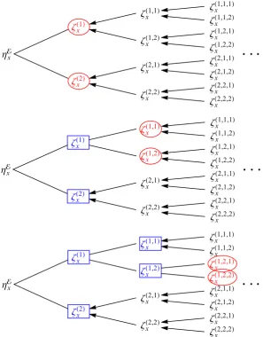
Letm≥2b_{be the smallest integer greater than or equal to the maximal jump rateg(2) = 2}b_(2.3) of the zero range process. The coupling as described below is applied for all timest ≥ 0 and sites x= 1, . . . , L−1, and is illustrated in Figure 1 for the simplest casem= 2. To each sitexwe associate an infinite number of birth-death chains(ζk

This corresponds to indexing the chains by the nodes of anm-ary regular treeRmwithout root, with generations indexed byn, and we writek∈ Rm. At any given time, each chainζxk(t)in the tree1)is an identical copy of its unique parent chain,2)evolves independently ofηx(t)and all other chains, or

3)is associated toηx(t)as described below. The assignment of each chain to one of these three groups changes in time, and we denote by

Cx(t) :=k∈ Rm:ζxk(t)is associated toηx(t), and no ancestor ofζxk(t)is associated toηx(t) Ix(t) :=

k∈ Rm:ζxk(t)evolves independently (5.8)

the index sets of chains which are not identical copies of their parent. At any timet≥0, the number of chains inCx(t)is|Cx(t)|=m, for all sitesx.

Initially, we set themchains in generationn= 1equal toηx, i.e.Cx(0) ={(1), . . . ,(m)},Ix=∅ and all other chains are identical copies of their parent. We use identical initial conditions, that is, for each sitex

ζ_x(1)(0) =. . .=ζ_x(m)(0) =ηx(0)∈ {0,1, . . . , βL}, (5.9) and our coupling will ensure that ηx(t) ≤ ζxk(t)for all k ∈ Cx(t). For the departure process of associated chains withk ∈ Cx(t)we simply use a basic coupling for allxandt ≥ 0, i.e. particles inζ_xk(t)leave together with particles inηx(t)with probabilityg ζxk(t)

/g ηx(t)

≤1forηx(t)>1, and they additionally leave, independently of particles inηx(t), at rateg ζxk(t)

−g ηx(t)in case this quantity is positive forηx(t)≤1. Note that the departure dynamics preserve the order

ηx(t)≤ζxk(t) for allk∈ Cx(t)andt≥0, (5.10) and we will couple the arrival processes in such a way that this is true also for the full process. To achieve this, we change the structure summarized by the setsCx(t)andIx(t)at every jump event on the arrival site. When a particle arrives at sitexin theη-process at timetwe pick one of themchains in

Cx(t)uniformly at random, add a particle to all of itsmchildren (which up to this point have evolved as identical copies of their parent), and disassociate the chains inCx(t−)so that from this time on they run independently ofηx(s), s≥t. That is, samplek∗∼U(Cx(t)), and let

Cx(t) =

(k∗,1),(k∗,2), . . . ,(k∗, m) , Ix(t) =Ix(t−)∪ Cx(t−).

So far the coupling leads to an effective arrival rate ofax(η(t))/m≤1,ax(η(t))as in (5.7), for each associated chain, which is typically strictly smaller than1. To each associated process we independently add particles at rate1−ax(η(t))/m, leading to a total arrival rate of1as required. Therefore all chains

(ζk

x(t) : t ≥0),k ∈ Rm, have the desired marginal dynamics of a birth-death chain with generator (5.1). Note that the total number of particles in the associated chains is not conserved and is growing in time, but the main point is that the coupling fulfills (5.10).

This coupling construction leads to increasing setsIx(t)of independently evolving chains, but at any time there is only a finite number of chains which are not identical copies of their parent. This number grows only linearly in time with high probability, and we will use this in the next subsection to prove a uniform bound on the exit rate from a well.

5.2

Proof of Lemma 3.5