Manuscript version: Author’s Accepted Manuscript
The version presented in WRAP is the author’s accepted manuscript and may differ from the published version or Version of Record.
Persistent WRAP URL:
http://wrap.warwick.ac.uk/129550
How to cite:
Please refer to published version for the most recent bibliographic citation information. If a published version is known of, the repository item page linked to above, will contain details on accessing it.
Copyright and reuse:
The Warwick Research Archive Portal (WRAP) makes this work by researchers of the University of Warwick available open access under the following conditions.
Copyright © and all moral rights to the version of the paper presented here belong to the individual author(s) and/or other copyright owners. To the extent reasonable and
practicable the material made available in WRAP has been checked for eligibility before being made available.
Copies of full items can be used for personal research or study, educational, or not-for-profit purposes without prior permission or charge. Provided that the authors, title and full
bibliographic details are credited, a hyperlink and/or URL is given for the original metadata page and the content is not changed in any way.
Publisher’s statement:
Please refer to the repository item page, publisher’s statement section, for further information.
Dynamic Multiscale Spatiotemporal Models
for Poisson Data
Tha´ıs C. O. Fonseca1 and Marco A. R. Ferreira2
Abstract
We propose a new class of dynamic multiscale models for Poisson spatiotemporal pro-cesses. Specifically, we use a multiscale spatial Poisson factorization to decompose the Pois-son process at each time point into spatiotemporal multiscale coefficients. We then connect these spatiotemporal multiscale coefficients through time with a novel Dirichlet evolution. Further, we propose a simulation-based full Bayesian posterior analysis. In particular, we develop filtering equations for updating of information forward in time and smoothing equa-tions for integration of information backward in time, and use these equaequa-tions to develop a forward filter backward sampler for the spatiotemporal multiscale coefficients. Because the multiscale coefficients are conditionally independent a posteriori, our full Bayesian pos-terior analysis is scalable, computationally efficient, and highly parallelizable. Moreover, the Dirichlet evolution of each spatiotemporal multiscale coefficient is parametrized by a discount factor that encodes the relevance of the temporal evolution of the spatiotemporal multiscale coefficient. Therefore, the analysis of discount factors provides a powerful way to identify regions with distinctive spatiotemporal dynamics. Finally, we illustrate the useful-ness of our multiscale spatiotemporal Poisson methodology with two applications. The first application examines mortality ratios in the state of Missouri, and the second application considers tornado reports in the American Midwest.
Keywords: Areal data; Bayesian dynamic models; Massive data sets; MCMC; Multiscale
modeling; Time series models for counts.
1
Introduction
Advances in data acquisition technology have led to an explosive increase in the size of
scientific data sets. This in turn has led to the need of statistical methods that scale well with
data set size. Several methods have been proposed for the analysis of large Gaussian
point-referenced data sets (e.g., Fuentes, 2007; Banerjee et al., 2008; Paciorek and McLachlan,
2009; Lemos and Sans´o, 2009). With respect to areal data (e.g., Banerjee et al., 2004),
several spatiotemporal models and methods have been developed for disease mapping (e.g.,
see Bernardinelli et al., 1995; Waller et al., 1997; Knorr-Held, 2000; Schmid and Held, 2004;
Tzala and Best, 2008, and references therein). However, these models and methods usually
do not scale well with data set size. A possible way to develop methods that scale well for
large data sets is through multiscale spatiotemporal models, such as the models for Gaussian
data developed by Berliner et al. (1999), Johannesson et al. (2007), and Ferreira et al. (2010,
2011); however, their methodology is not directly applicable to Poisson data. Here, we
propose a new class of dynamic multiscale models for Poisson spatiotemporal processes.
To develop new dynamic multiscale spatiotemporal Poisson (MSSTP) models, we couple
a multiscale Poisson factorization with a novel Dirichlet temporal evolution. Specifically,
at each time point we apply the Kolaczyk-Huang multiscale spatial Poisson factorization
(Kolaczyk and Huang, 2001) to decompose the mean or intensity function of the Poisson
process into spatiotemporal multiscale coefficients. Further, we connect the spatiotemporal
multiscale coefficients through time with a novel Dirichlet temporal evolution. This temporal
evolution is related to conditionally conjugate temporal evolution for binomial, negative
binomial, Poisson, and multinomial observations (Smith, 1979, 1981) (see also Harvey, 1989;
Prado and West, 2010; Gamerman et al., 2013). Our novel Dirichlet temporal evolution
depends on discount factors related to how fast the spatiotemporal multiscale coefficients
change through time.
For the analysis of these new dynamic MSSTP models, we propose a simulation-based
information forward in time and smoothing equations for integration of information
back-ward in time. We then use these filtering and smoothing equations to develop a forback-ward
filter backward sampler for the spatiotemporal multiscale coefficients. Further, we provide
marginal posterior densities for the discount factor parameters. Hence, to simulate from the
joint posterior distribution of all the unknown quantities in the model, we use a composite
approach. First, we simulate a sample of the discount factor parameters from their marginal
posterior distributions. After that, for each simulated discount factor we simulate a
realiza-tion of the spatiotemporal multiscale coefficients using our forward filter backward sampler.
As a result, we obtain a sample from the joint posterior distribution of discount factors and
spatiotemporal multiscale coefficients.
Research on multiscale spatiotemporal models is in its infancy, and the relatively few
arti-cles published to date focus on Gaussian data. Berliner et al. (1999) developed a hierarchical
model for turbulence using a wavelet decomposition for an underlying latent turbulence
pro-cess and allowed the wavelet coefficients to evolve through time using state-space equations.
Johannesson et al. (2007) have proposed a multiscale decomposition that uses a coarse to
fine construction, assumes a fixed number of children subregions at each resolution level, and
assumes temporal dynamics only at the aggregated coarse level. More recently, Ferreira et al.
(2010, 2011) have developed multiscale spatiotemporal models based on a non-wavelet-based
multiscale decomposition that allows a different number of children for each subregion at any
resolution level, allows non-constant variance across the region of interest, and assumes
tem-poral dynamics at all scales of resolution. However, these previous multiscale spatiotemtem-poral
models are not directly applicable to Poisson data.
Our MSSTP methodology decomposes large Poisson data sets into many smaller
com-ponents called empirical multiscale coefficients. For inhomogeneous spatiotemporal Poisson
processes, given the latent spatiotemporal multiscale coefficients, the empirical multiscale
coefficients are conditionally independent. Further, we assume a separate Dirichlet temporal
latent coefficients are conditionally independent a priori. As a result, the multiscale Poisson
factorization of the likelihood function leads the spatiotemporal multiscale coefficients to
be conditionally independent a posteriori. As a practical consequence, each spatiotemporal
multiscale coefficient and its corresponding discount factor can be analyzed separately,
lead-ing our full Bayesian posterior analysis to be scalable, computationally efficient, and highly
parallelizable.
Our multiscale spatiotemporal framework performs smoothing simultaneously in space
and time. This point is made clear in Section 4, where we present results on the spatial
and spatiotemporal dependence structures of our proposed models. To further investigate
this point, Section 5.3 presents for two real data applications a comparison of our MSSTP
model to two competing models. First, to access the ability of our MSSTP framework
to borrow strength spatially, we compare our model to a model that assumes that each
finest level subregion has its own temporal evolution. Second, to access our framework’s
ability to incorporate spatiotemporal dynamics, we compare our model to a widely used
spatiotemporal model based on Markov random fields. We perform these model comparisons
using two criteria: the conditional Bayes factor (e.g., see Ghosh et al., 2006; Vivar and
Ferreira, 2009) that compares the predictive performance of the competing models, and the
deviance information criterion (DIC) (Spiegelhalter et al., 2002). As Section 5.3 reports, for
both applications our MSSTP model is substantially superior to the two competing models.
Therefore, by borrowing strength spatially and by incorporating spatiotemporal dynamics,
our MSSTP model for Poisson data provides superior results.
We advocate the analysis of the discount factors as a powerful way to identify regions
with important spatiotemporal dynamics. Specifically, as spatiotemporal data sets grow
increasingly larger, it is not feasible to visualize the entire data set. Our MSSTP framework
offers great opportunity in terms of prioritizing what subregions of the region of interest
should be analyzed more thoroughly. In particular, each discount factor is related to how
each discount factor encodes the relevance of the temporal evolution of the corresponding
spatiotemporal multiscale coefficient. Therefore, smaller discount factors indicate regions
where the mean or intensity function changes more rapidly through time and thus contain
spatiotemporal dynamics that warrant further investigation.
The remainder of this article is organized as follows. Section 2 describes the Poisson
mul-tiscale factorization and introduces the proposed dynamic mulmul-tiscale spatiotemporal model
for Poisson data. Section 3 develops a simulation-based full Bayesian posterior analysis
methodology. Section 4 presents results on the spatial and spatiotemporal dependence
struc-tures of our proposed models. Section 5 illustrates the usefulness of our novel methodology
with applications to two real data sets. Finally, Section 6 presents conclusions and future
developments. For convenience of exposition, we present all proofs in the Appendix.
2
Multiscale Poisson spatiotemporal modeling
To develop new dynamic multiscale models for Poisson spatiotemporal processes, we couple
a multiscale Poisson factorization with a novel Dirichlet temporal evolution. Specifically, at
each time point we apply the multiscale spatial Poisson factorization proposed by Kolaczyk
and Huang (2001) to decompose the mean or intensity function of the Poisson process into
spatiotemporal multiscale coefficients. In addition, we apply the same factorization to the
Poisson data set and obtain empirical spatiotemporal multiscale coefficients that are na¨ıve
estimators of the latent spatiotemporal multiscale coefficients. For completeness and to
establish notation, Section 2.1 presents the multiscale factorization of Kolaczyk and Huang
(2001) (see also Ferreira and Lee, 2007, Chapter 9) that we specialize for spatiotemporal
Poisson data. After that, Section 2.2 describes the temporal evolution of the mean process
at the coarsest resolution level and of the spatiotemporal multiscale coefficients at the various
resolution levels. Finally, in Section 2.3 we complete our MSSTP model for Poisson areal
2.1
Poisson multiscale factorization
Assume that interest lies in an inhomogeneous spatiotemporal Poisson process with rate
{λt(s) : s ∈ S, t ∈ Z} on a spatial domain S ⊂ Rk. Here, k is typically less than or
equal to 3. Moreover, assume that because of measurement, resources or confidentiality
restrictions, data are available only up to a given scale of resolution L on a partition of
the domain S. Denote this partition by {BL1, . . . , BL,nL}, with BLj ∈ S, j = 1, . . . , nL,
BLi ∩BLj = ∅, i 6= j, and ∪nj=1L BLj = S. For example, because of confidentiality concerns
data on occurrences of a disease may only be available at the county level; in this case,
BL1, . . . , BL,nL would be the counties within the domain S. On another example, when
considering point process data, because of limitations of computational resources it may be
more advantageous to bin the data. In this case, BL1, . . . , BL,nL would be the bins at the
finest resolution level. We illustrate this latter case with the tornado report application
presented in Section 5.2.
For each subregion BLj there is a count ytLj of the number of occurrences of the event of
interest at time t, t = 1, . . . , T. Moreover, the expected number of counts on BLj at time t
is µtLj =E(ytLj) =
R
BLjλt(s)ds, j = 1, . . . , nL. Then, the model for the number of counts
at the finest resolution level Lat time t is
ytLj|µtLj ∼Poisson(µtLj). (1)
Further, similarly to Kolaczyk and Huang (2001) we assume that ytL1, . . . , ytL,nL are
con-ditionally independent given µtL1, . . . , µtL,nL, t = 1, . . . , T. In what follows, the latent
spa-tiotemporal process λt(s) is constructed in a way that this latent process will be
spatiotem-porally correlated. Therefore, this spatiotemporal dependence will transfer to the counts
ytL1, . . . , ytL,nL and lead their marginal distribution to contain spatiotemporal dependence.
In addition to the mean process at the Lth resolution level, we are also interested in
the process at aggregated coarser scales. At the lth scale of resolution, the domain S is
is assumed to be a refinement of the partition at level l+ 1; that is, Blj =∪(l+1,j0)∈D
ljBl+1,j0, where Dlj is the set of descendants of subregion j at level l, and Dlj ∩ Dli = ∅, i 6= j.
Additionally, let Al(L, j) be the ancestor at resolution level l of subregion (L, j). Finally,
denote by dlj the number of descendants of subregion (l, j).
We assume that we observe data at the finest resolution levelLand aggregate the data to
obtain the data at resolution levels 1 toL−1. LetGbe a set of subregions and denote byytG
andµtG the corresponding vectors of counts and expected values at timet, respectively. For
example, ytDlj denotes the vector of counts observed in the descendants of subregion (l, j)
at time t. Further, let 1m denote the m-dimensional vector of ones. Then, the aggregated
counts at the lth level of resolution at time t are recursively defined as ytlj =10dljytDlj with
corresponding aggregated mean process µtlj = 10dljµtDlj. Usually, the mean µtlj may be
written as µtlj = λtljetlj, where λtlj is the relative risk on subregion (l, j) at time t and etlj
is either known or unknown up to a low-dimensional parameter vector. Examples of known
etlj include the case when etlj = 1 and the case when etlj is the known population size of
subregion (l, j) at time t. We illustrate these two cases of known etLj with the application
presented in Section 5.1. In contrast, an example of etLj unknown up to a low-dimensional
parameter vector is etLj = exp(x0tβLj), where xt is a known vector of regressors common
to all regions at time t and βLj = βA1(L,j), and we recall that Al(L, j) is the ancestor
at resolution level l of subregion (L, j). We demonstrate this latter case of unknown etLj
with the application presented in Section 5.2. Similarly to the observed counts, etlj may be
aggregated as etlj = 10dljetDlj. In that case, the aggregation for the mean process implies
that the relative risk process is aggregated as λtlj =e−tlj1λ 0
tDljetDlj.
We now apply the Poisson multiscale factorization of Kolaczyk and Huang (2001) to
the intensity function and to the data at time t. Because the observations at the finest
distributions, the likelihood function admits the multiscale factorization
nL Y
j=1
p(ytLj|µtLj) = n1 Y
j=1
p(yt1j|µt1j) L−1
Y
l=1
nl Y
j=1
p(ytDlj|ytlj,ωtlj), (2)
where yt1j|µt1j ∼ Poisson(µt1j). Further, ytDlj|ytlj,ωtlj ∼ Multinomial(ytlj,ωtlj), where
ytlj plays the role of the sample size parameter of the multinomial distribution, and
ωtlj = µtDlj/µtlj is the vector of probabilities. Hence, ωtlj describes how the counts ytlj
at subregion (l, j) at time t are expected to be distributed among the descendants in
Dlj. Because ωtlj connects coarser to finer resolution levels, in analogy to wavelet
anal-ysis (Vidakovic, 1999) we refer to ωtlj as the spatiotemporal multiscale coefficient.
Fi-nally, note that the factorization (2) reparameterizes the Poisson model initially
parame-terized by the mean process at the finest level µtL,1:n
L in terms of the mean process at
the coarsest level and the multiscale coefficients that connect the several resolution levels
(µt1,1:n1,ωt1,1:n1, . . . ,ωt,L−1,1:nL−1).
LetD0 denote the information available at time t= 0 and recursively defineDt=Dt−1∪
{yt} to be the information available up to time t. We follow the terminology used by West
and Harrison (1997) for describing the propagation of information through time. Specifically,
the distribution of µtlj given the data up to time t−1, p(µtlj|Dt−1), is referred to as the
prior distribution. After incorporating the data observed at time t, p(µtlj|Dt) is referred to
as the posterior or filtered distribution. Finally, the distribution of µtlj conditional on the
data observed at all time points, p(µtlj|DT), is referred to as the smoothing distribution.
2.2
Temporal evolution
This section describes the temporal evolution of the mean process at the coarsest resolution
level and of the spatiotemporal multiscale coefficients at the various resolution levels.
At the coarsest levell = 1, we have the aggregated observationsyt1,1:n1 = (yt11, . . . , yt1n1).
that the aggregated observations also have a Poisson distribution, that is
yt1j|µt1j ∼Poisson(µt1j), j = 1, . . . , n1. (3)
We are interested in making inference for the relative risk at region (1, j) at timet which
is defined as λt1j = µt1j/et1j, where et1j is the expected number of counts at region (1, j)
and time t. The expected countet1j might be assumed known or estimated using covariates
by et1j = exp{x0tjβj}, where xtj is a vector of covariates and βj is a vector of unknown
regression coefficients. For the stochastic temporal evolution of the coarse level relative risk
λt1j,j = 1, . . . , n1, we assume the beta temporal evolution first proposed by Smith and Miller
(1986) in the context of space models for univariate Poisson observations. Other
state-space models for Poisson observations could be used as well, such as for example dynamic
generalized linear models (West et al., 1985; Ferreira and Gamerman, 2000). However, here
we are concerned with speed and scalability of computations and the model of Smith and
Miller (1986) leads to fast conjugate-analysis filters and samplers. The following definition
adapts the model of Smith and Miller (1986) to our context.
Definition 2.1 (Beta evolution for coarse level risk) Let ηtj|Dt−1, γj ∼ Beta(γjat−1,j,
(1−γj)at−1,j), where 0< γj ≤ 1 is a discount factor parameter, and at−1,j >0. Then, the
beta temporal evolution for λt1j is defined as
λt1j =λt−1,1jγj−1ηtj. (4)
From the first and second moments of the beta distribution, we obtainE(γj−1ηtj|Dt−1, γj) =
1 and V ar(γj−1ηtj|Dt−1, γj) = (γj−1 −1)/(at−1,j + 1). Thus, the closer γj is to one and the
larger the value of at−1,j, the closer λt1j will be to λt−1,1j. Further, as we discuss in
Sec-tion 3.1, atj summarizes the information up to time t about λt1j. In addition, the discount
factorγj provides the rate of information loss from time t−1 to timet about the risk for the
coarse level subregion (1, j). Finally, the discount factorγj will be estimated thus providing
Now let us consider the temporal evolution of the spatiotemporal multiscale coefficients
at levels of resolution l = 1, . . . , L−1. Recall that ωtlj = µtDlj/µtlj is the spatiotemporal
multiscale coefficient that connects the mean process at subregion (l, j) to the mean process
at its descendants at time t. Further, let ωetlj =ytDlj/ytlj be an estimator of ωtlj. We refer
to ωe
tlj as the empirical spatiotemporal multiscale coefficient for subregion (l, j) at time t.
The multiscale decomposition given in Equation (2) implies for ytDlj =ytljω
e
tlj the model
ytljωetlj|ytlj,ωtlj ∼Multinomial(ytlj,ωtlj). (5)
Definition 2.2 below describes our novel Dirichlet temporal evolution for the
spatiotem-poral multiscale coefficient ωtlj. Let denotes the Hadamard product (p. 45, Magnus and
Neudecker, 1999), that is, the operation that returns the vector of element-wise products.
As we establish in Theorem 3.3, Definition 2.2 implies an integration of information forward
in time based on the Dirichlet distribution.
Definition 2.2 (Dirichlet evolution for spatiotemporal multiscale coefficients) Let
φtlj = (φtlj1, . . . , φtlj,dlj)
0
, whereφtlj1, . . . , φtlj,dlj are independent withφtlji ∼Beta(δljct−1,lji,(1−
δlj)ct−1,lji), Stlj = φ0tljωt−1,lj, 0 < δlj ≤ 1 is a discount factor parameter, and ct−1,lji > 0,
i= 1, . . . , dlj. Then, the Dirichlet temporal evolution for ωtlj is defined as
ωtlj =
1
Stlj
φtljωt−1,lj. (6)
As it will become clear in Section 3.1,ctlj = (ctlj1, . . . , ctlj,dlj) summarizes the information
up to timet about ωtlj. Moreover, the discount factor δlj, which will be estimated from the
data, provides the rate of information loss from timet−1 to timetabout the spatiotemporal
multiscale coefficient for subregion (l, j). Other state-space models for multinomial
observa-tions could be used for the evolution of ωtlj, such as for example the conditionally Gaussian
dynamic models of Cargnoni et al. (1997). This would allow the inclusion of covariates at
multiple scales of resolution, and variable selection in that context may be performed using
proceeding and will be reported elsewhere. However, here we prefer our Dirichlet temporal
evolution that leads to a conjugate-analysis-based forward filter and backward sampler that
is computationally fast and scalable.
2.3
Initial conditions and priors for the discount factors
We complete our proposed MSSTP model for Poisson areal data by specifying the priors for
the discount factors and for the latent process at time t = 0.
The priors for the latent process at time t= 0 represent the initial information about the
process before obtaining any observation. For the latent mean process at the coarsest level of
resolution λ01j, j = 1, . . . , n1, we assume conditionally independent conjugate gamma prior
distributionsλ01j|D0 ∼Gamma(a0j, b0j),j = 1, . . . , n1, wherea0j >0 andb0j >0 are known
and represent the prior information at time t = 0 about λ01j. The prior mean and variance
of λ01j are a0j/b0j and a0j/b20j respectively. Typically, a0j and b0j are chosen to be small
values to indicate vague prior information.
For the latent spatiotemporal multiscale coefficient for subregion (l, j) at timet = 0,ω0lj,
j = 1, . . . , nj, we assume conditionally independent conjugate Dirichlet prior distributions
ω0lj|D0 ∼Dirichlet(c0lj), where c0lj is a known vector with elements c0lji>0, i= 1, . . . , dlj.
The vector c0lj represents the prior information about ω0lj. Typically, the elements of c0lj
are chosen to be small values to indicate vague prior information.
Similarly to discount factors in Gaussian state-space models (West and Harrison, 1997),
the discount factors in our proposed model describe the loss of information through time
before the next observation is obtained. The discount factors are parameters that may
assume values in the interval (0,1). As we discuss in Section 3, a discount factor close to
1 indicates a smaller rate of loss of information through time and therefore a more stable
latent process. Because discount factors belong to the interval (0,1), we assume for them
beta prior distributions. Specifically, we assumea prioriγj ∼Beta(aγ, bγ), j = 1, . . . , n1, and
of the discount factor priors are aγ = bγ = 1 and aδ = bδ = 1 which imply noninformative
uniform priors on the interval (0,1).
3
Posterior Analysis
In this section we develop simulation-based Bayesian posterior analysis for our proposed
MSSTP model for Poisson data. The first two sections, 3.1 and 3.2, consider the case when
the discount factors and regression coefficients are fixed. Specifically, Section 3.1 presents
results for temporal filtering, that is, the updating of information through time for λt1j and
ωtlj. In addition, Section 3.2 presents results for spatiotemporal smoothing, that is, the
integration of spatiotemporal information backward in time. For the case when the discount
factors and the regression coefficients are unknown, Section 3.3 presents their marginal
pos-terior distributions. Finally, Section 3.4 introduces algorithms for the implementation of
simulation-based full Bayesian posterior analysis.
The following theorem states that the posterior analysis of our MSSTP model may be
broken down into many independent parts. As a result, the analysis may be implemented
with a divide-and-conquer strategy that leads to a highly parallelizable algorithm.
Theorem 3.1 Consider the MSSTP model defined by Equations (1), (2), (3), (4), (5), and
(6). Given the discount factor parameters γj, j = 1, . . . , n1, and δlj, l = 1, . . . , L−1, j =
1, . . . , nl, the vectorsλ1:T,11, . . . ,λ1:T,1n1,ω1:T ,11, . . . ,ω1:T,1n1,. . .,ω1:T ,L−1,1, . . . ,ω1:T,L−1,nL−1
are conditionally independent a posteriori.
In what follows, we present results and algorithms for the simulation of the parameters
γ1, . . . , γn1, δ11, . . . , δ1n1, . . ., δL−1,1, . . . , δL−1,nL−1, λ1:T ,11, . . . ,λ1:T,1n1, ω1:T,11, . . . , ω1:T,1n1,
3.1
Temporal filtering
This section presents results on temporal filtering forλ1:T ,1j andω1:T ,lj. First, let us consider
filtering for λ1:T ,1j. As explained in Section 2.3, at time t = 0 we assume the distribution
λ01j|D0 ∼Gamma(a0j, b0j). Then, Theorem 3.2 provides the filtering equations for λ1:T ,1j.
Theorem 3.2 Assume the initial distribution λ01j|D0 ∼ Gamma(a0j, b0j) and consider the
Observation Equation (3) and the beta temporal evolution for λt1j given by Equation (4) in
Definition 2.1. Then, for t= 1, . . . , T:
(i) Posterior for λt−1,1j: λt−1,1j|Dt−1, γj,βj ∼Gamma(at−1,j, bt−1,j).
(ii) Prior for λt1j: λt1j|Dt−1, γj,βj ∼Gamma(at|t−1,j, bt|t−1,j),
where at|t−1,j =γjat−1,j and bt|t−1,j =γjbt−1,j.
(iii) Posterior for λt1j: λt1j|Dt, γj,βj ∼Gamma(atj, btj),
where atj =γjat−1,j+yt1j and btj =γjbt−1,j+et1j.
Hence, atj and btj, t = 1, . . . , T, are recursively computed based on Theorem 3.2
and summarize the information about λt1j up to time t. Note that the prior mean
E(λt1j|Dt−1, γj) is equal to E(λt−1,1j|Dt−1, γj) while the prior variance V(λt1j|Dt−1, γj) is
equal toγj−1V(λt−1,1j|Dt−1, γj). Thus, the discount factor parameterγj inflates the variance
from timet−1 to timetby a factor equal to γj−1. Therefore, values ofγj closer to one imply
a smaller rate of information loss through time and therefore a more stable latent process.
Finally, in the limit when γj →1 the latent process {λt1j}would be constant through time.
From the posterior distributionλt1j|Dt, γj, βj, it follows that an estimator of λt1j at time
t is given by the filtered posterior mean E(λt1j|Dt, γj,βj) = (γjat−1,j+yt1j)/(γjbt−1,j+et1j)
and a measure of uncertainty is given by the filtered posterior varianceV ar(λt1j|Dt, γj,βj) =
(γjat−1,j+yt1j)/(γjbt−1,j+et1j)2.
Now let us consider filtering for ω1:T ,lj. First, recall from Section 2.3 that the initial
distribution for ω0lj at time t = 0 is ω0lj|D0 ∼Dirichlet(c0lj). Then, Theorem 3.3 provides
Theorem 3.3 Assume the initial distribution ω0lj|D0 ∼ Dirichlet(c0lj), and consider the
Observation Equation (5) and the Dirichlet evolution for the spatiotemporal multiscale
coef-ficient ωtlj given by Equation (6) in Definition 2.2. Then, for t= 1, . . . , T:
(i) Posterior for ωt−1,lj: ωt−1,lj|Dt−1, δlj ∼Dirichlet(ct−1,lj).
(ii) Prior for ωtlj: ωtlj|Dt−1, δlj ∼Dirichlet(ct|t−1,lj), where ct|t−1,lj =δljct−1,lj.
(iii) Posterior for ωtlj: ωtlj|Dt, δlj ∼Dirichlet(ctlj), where ctlj =δljct−1,lj+ytljωetlj.
Hence, ctlj,t= 1, . . . , T, are recursively computed based on Theorem 3.3 and summarize
the information up to time t about the spatiotemporal multiscale coefficient ωtlj. From
Theorem 3.3, it follows that E(ωtlj|Dt−1, δlj) = E(ωt−1,lj|Dt−1, δlj) = ct−1,lj/ (10dljct−1,lj),
where dlj is the number of descendants of subregion (l, j). Thus, conditional on the data
up to time t−1 the expected value of ωtlj is equal to that of ωt−1,lj. Moreover, the prior
covariance matrix of ωtlj is
V(ωtlj|Dt−1, δlj) =δlj−1 10d
ljct−1,lj+ 1
10d
ljct−1,lj+δ
−1
lj
V(ωt−,lj|Dt−1, δlj).
Hence, similarly to γj, the discount factor δlj impacts the information flow through time
by inflating the covariance matrix of ωtlj by a factor that, for large values of 10dljct−1,lj, is
approximately equal to δlj−1. Therefore, values of δlj closer to one imply a smaller rate of
information loss through time and therefore a more stable latent spatiotemporal multiscale
coefficient. Finally, from Theorem 3.3 it follows that an estimator of ωtlj at time t is given
by the filtered or posterior mean E(ωtlj|Dt, δlj) = (δljct−1,lj+ytljωetlj)/(δlj1d0ljct−1,lj+ytlj).
3.2
Temporal smoothing
This section presents results on temporal smoothing for λ1:T ,1j and ω1:T,lj. First, let us
Proposition 3.1 Assume the Observation Equation (3) and the beta temporal evolution for
λt1j given by Equation (4) in Definition 2.1. Then, the conditional smoothing distribution of
λt−1,1j given λt1j is equal to
p(λt−1,1j|DT, λt1j, γj) =
b(1−γj)at−1,j
t−1,j
Γ((1−γj)at−1,j)
(λt−1,1j −γjλt1j)(1−γj)at−1,j−1 (7)
×exp{−bt−1,j(λt−1,1j−γjλt1j)}, λt−1,1j −γjλt1j >0.
We use Proposition 3.1 to develop a backward sampling scheme for λt1j that is described
in Algorithm 3.1.
Let us now consider smoothing for the spatiotemporal multiscale coefficientω1:T ,lj. Recall
from Equation (6) that the auxiliary variableStlj is defined asStlj =P dlj
i=1φtljiωt−1,lji. Then,
the following proposition provides a way to simulate from the joint distribution of Stlj and
ωt−1,lj.
Proposition 3.2 Consider the Observation Equation (5) and the Dirichlet temporal
evolu-tion for the spatiotemporal multiscale coefficient ωtlj given by Equation (6) in Definition 2.2.
Then,
(i) ωt−1,lj|DT, Stlj,ωtlj, δlj ∼Mod-Dirichlet((1−δlj)ct−1,lj, Stljωtlj)
(ii) Stlj|DT,ωtlj, δlj ∼Beta(δljc˜t−1,lj,(1−δlj)˜ct−1,lj)
where c˜t−1,lj = P dlj
i=1ct−1,lji and Mod-Dirichlet denotes the modified Dirichlet distribution
defined in Definition A.1.
We use Proposition 3.2 to develop a backward sampling scheme forω1:T ,ljthat is described
in Algorithm 3.2.
3.3
Marginal posterior distributions for hyperparameters
This section presents the marginal posterior distributions for the discount factors γ1:n1,
At the coarsest levell= 1, the Poisson-gamma model implies a negative binomial
predic-tive distribution for the coarse level observations. The likelihood function for the discount
factor γj and the regression coefficientsβj, j = 1, . . . , n1 is
p(y1:T ,1j|γj,βj,D0) =
T
Y
t=1
p yt1j|Dt−1, γj,βj
= T Y t=1 Z ∞ 0
p yt1j|γj,βj, λt1j
p λt1j|Dt−1, γj,βj
dλt1j
=
T
Y
t=1
Γ(γjat−1,j+yt1j)
Γ(γjat−1,j)Γ(yt1j + 1)
γjbt−1,j
ex0tjβj
γjat−1,j
1 + γjbt−1,j
ex0tjβj
−(γjat−1,j+yt1j))
. (8)
Therefore, by Bayes Theorem the marginal posterior distribution for (γj,βj) is given by
p(γj,βj|DT)∝p(y1:T ,1j|D0, γj,βj)p(γj,βj).
The multinomial-Dirichlet model implies that the likelihood function for the finer
reso-lution discount factors δlj, l= 1, . . . , L−1,j = 1, . . . , nl, is given by
p(y1:T ,Dlj|D0,y1:T ,lj, δlj) =
T
Y
t=1
p(yt,Dlj|Dt−1, ytlj, δlj)
=
T
Y
t=1
Z
p(yt,Dlj|ytlj,ωtlj)p(ωtlj|Dt−1, δlj)dωtlj
= T Y t=1 Γ(P
iδljct−1,lji)Γ(ytlj+ 1)
Γ(P
iδljct−1,lji+ytlj) dlj
Y
i=1
Γ(δljct−1,lji+ytljωtljie )
Γ(ytljωetlji+ 1)Γ(δljct−1,lji)
. (9)
Therefore, by Bayes Theorem the marginal posterior distribution for δlj is p(δlj|DT) ∝
p(y1:T ,Dlj|D0,y1:T ,lj, δlj)p(δlj).
Because we assumea0 >0,b0 >0, andc0 >0 (see Section 2.3), the densities that appear
in Equations (8) and (9) are always proper. In that case, the products in those equations
and b0 = 0, then the products in Equation (8) have to start from the first time τ for which
p λτ1j|Dτ−1, γj,βj
is a proper density. Similarly, if the practitioner uses improper priors
with c0 = 0 then the products in Equation (9) have to start from the first time τ for which
p(ωτ lj|Dτ−1, δlj) is a proper density.
3.4
Posterior simulation
This section presents algorithms for the simulation from the joint posterior distribution
of the parameters of our MSSTP model for Poisson data defined by Equations (1), (2),
(3), (4), (5), and (6). Note that as a result of Theorem 3.1, simulation from the
joint posterior distribution may be broken down into many independent parts.
Specifi-cally, simulation of (γ1,β1,λ1:T ,1), . . ., (γn1,βn1,λ1:T,n1), (δ1,1,ω1:T,1,1), . . ., (δ1,n1,ω1:T ,1,n1),
. . ., (δL−1,1,ω1:T,L−1,1), . . ., (δL−1,nL−1,ω1:T ,L−1,nL−1), may be performed in parallel. As a consequence, each draw from the posterior distribution has computations of the order
O(T{n1+P
L−1
l=1
Pnl
j=1dlj}), which is typically substantially smaller than the computations
of the orderO(T n3
L) associated with a spatiotemporal model based on state-space equations
with a full system equation covariance matrix. Finally, the use of a parallel machine with
number of nodes larger than the number of spatiotemporal multiscale coefficients will have
computational time of the order O(T maxl,jdlj).
At the coarsest level of resolution, sampling from p(γj,βj,λ1:T ,1j|DT), j = 1, . . . , n1,
may be performed through a composite sampling algorithm. First, we sample (γj,βj) from
the marginal posterior distribution p(γj,βj|DT) using a Metropolis-Hastings within Gibbs
algorithm. After that, for the draws of (γj,βj) obtained after convergence, we sample λ1:T,1
fromp(λ1:T ,1|γ,β,DT). This latter part is performed with a forward filter backward sampler
scheme that we describe below.
Algorithm 3.1 (Forward Filter Backward Sampler forλ1:T,j). To sample fromp(λ1:T ,j|DT, γj,βj),
1. Recursively compute the filtering distributions λt1j|Dt, γj,βj ∼ Gamma(atj, btj), t =
1, . . . , T, as given in Theorem 3.2.
2. Sample λT1j from λT1j|DT, γj,βj ∼Gamma(aT j, bT j).
3. For t from T to 2, recursively sample λt−1,1j from p(λt−1,1j|DT, λt1j, γj) which is
pre-sented in Proposition 3.1:
• Sampleu from Gamma((1−γj)at−1,j, bt−1,j);
• Set λt−1,1j =u+γjλt1j.
At the l-th level of resolution, sampling from p(δlj,ω1:T,lj|DT), l = 1, . . . , L − 1,
j = 1, . . . , nl, may be accomplished with a composite sampling algorithm. Because δlj is
one-dimensional and its prior distribution has compact support, we find that a
straightfor-ward sampling-importance-resampling algorithm works well in simulating from the marginal
posterior distribution of δlj. After that, for the draws of δlj obtained after convergence, we
sample ω1:T ,lj from p(ω1:T ,lj|δlj,DT). This latter part is performed with the novel forward
filter backward sampler scheme that we describe below.
Algorithm 3.2 (Forward Filter Backward Sampler for ω1:T,lj). To sample from
p(ω1:T,lj|DT, δlj), l = 1, . . . , L−1, j = 1, . . . , nl, we proceed as follows.
1. Recursively compute the filtering distributions ωtlj|Dt, δlj ∼ Dirichlet(ctlj), t =
1, . . . , T, as given in Theorem 3.3.
2. Sample ωT lj from ωT lj|DT, δlj ∼Dirichlet(cT lj).
3. For t from T to 2, recursively sample ωt−1,lj from p(ωt−1,lj|DT, St−1,lj,ωtlj,ωe1:T ,lj, δlj)
which is a Mod-Dirichlet((1−δl)ct−1,lj, sωtlj):
• SampleStljfromp(Stlj|DT,ωtlj,ωe1:T ,lj, δlj)which is aBeta(δlj˜ct−1,lj,(1−δlj)˜ct−1,lj)
• Sampleu from Dirichlet((1−δlj)ct−1,lj);
• Set ωt−1,lj =Stljωtlj+ (1−Stlj)u.
Frequently, we will be interested in making inference for the expected number of counts or
for the relative risk at subregion (l, j) at timetfor resolution levels finer than the coarsest
res-olution. Note that the algorithms in this section will provide a sample from the posterior
dis-tribution of (γ,β,δ,λ1:T,1, . . . ,λ1:T ,n1,ω1:T ,11, . . . ,ω1:T,1n1, . . . ,ω1:T ,L−1,1, . . . ,ω1:T ,L−1,nL−1). Then, a sample from the posterior distribution of the expected number of counts at the
coarsest resolution level can be obtained using the equality µt1j = λt1jet1j, t = 1, . . . , T,
j = 1, . . . , n1. After that, a sample from the posterior distribution of the expected
num-ber of counts at the various resolution levels can be obtained recursively with the equality
µtDlj = ωtljµtlj, t = 1, . . . , T, l = 1, . . . , L−1, j = 1, . . . , nl. In addition, draws from the
posterior distribution ofetlj can be easily obtained as functions of the simulated values ofβ.
Let denote the elementwise division operator. Finally, a sample from the posterior
distri-bution of the relative risk at the descendants of subregion (l, j) at time t can be obtained
with the equality λtDlj =µtDlj etDlj.
4
Spatiotemporal dependence structure
In this section we present the spatiotemporal dependence structure implied by the MSSTP
model we propose in Section 2. For simplicity of exposition, in this section we assumeet1j = 1
implying that µt1j = λt1j. In addition, we slightly abuse notation and denote by logv the
vector that results from applying the logarithm to each element of vector v. First we show
that, in the spirit of Bayesian dynamic models (West and Harrison, 1997), our MSSTP
model implies a spatiotemporal mean process at all resolution levels that is nonstationary.
In addition, to understand the spatial dependence structure, we provide results on the mean
vector and covariance matrix of logµt1,1:n1, logωtlj, and logµtl,1:nl conditional on Dt, the
mean process at the finest resolution level may be partitioned in two components: a common
temporal mean to all subregions that share the same coarsest level ancestor; and dynamic
spatiotemporal random effects that may be affected by distinct dynamics at specific regions
at multiple resolution levels. Finally, to better understand the spatiotemporal dependence
structure of our MSSTP model, we compare the implied dependence structure with that of
a widely used spatiotemporal model.
Let us consider the logarithm of the mean process. Note that Equation (4) implies the
temporal evolution logµt1j = logµt−1,1j+log(ηtj/γj), whereE(ηtj/γj) = 1 andV ar(ηtj/γj) =
(1−γj)/{γj(at−1,j + 1)}. Hence, the temporal evolution at the coarsest level of logµt1j
is a random walk. In addition, Equation (6) implies the temporal evolution logωtlj =
logωt−1,lj + log(φtlj /Stlj), where Stlj = ω0t−1,ljφtlj guarantees that 10dljωtlj = 1. Thus,
logωtlj follows a nonGaussian singular random walk (compare to Gaussian singular random
walks used by Ferreira et al., 2011). Note that the log-mean process may be disaggregated
from levellto levell+1 with the disaggregation equation logµtD
lj =1dljlogµtlj+logωtlj,l=
1, . . . , L−1. Because the temporal evolution of both the log-mean at the coarsest level and
the log spatiotemporal multiscale coefficients are random walks, the implied spatiotemporal
mean process at all resolution levels is nonstationary.
In addition, the disaggregation equation may be expanded to relate all the subregions at
levels l−1 and l as
logµtl,1:n
l =Bl−1logµt,l−1,1:nl−1 + logωt,l−1,1:nl−1, (10) where Bl−1 is an nl−1×nl block-diagonal matrix with jth diagonal block equal to a vector
of ones with length dDl−1,j and off-block-diagonal elements equal to zero. Even though our model is nonstationary, the vector of expectations and the covariance matrix of the
log-mean process at time t conditional on Dt, the information up to time t, are well defined.
In particular, Equation (10) may be used to recursively compute the vector of expectations
and the covariance matrix of the log-mean process at time t at all resolution levels. Let
We provide the recursive formulas for expectations and covariance matrices in the following
theorem.
Theorem 4.1 Consider the MSSTP model for Poisson data defined by Equations (1), (2),
(3), (4), (5), and (6). Then:
(i) E(logµt1,1:n1|Dt,γ) = (ψ(at1), . . . , ψ(atn1))
0−log(b
t1, . . . , btn1)
0.
(ii) Cov(logµt1,1:n1|Dt,γ) = diag(ψ0(at1), . . . , ψ0(atn1)).
(iii) E(logωtlj|Dt,δ) = (ψ(ctlj,1), . . . , ψ(ctlj,dlj))
0−ψ(10
dljctlj)1dlj.
(iv) Cov(logωtlj|Dt,δ) = diag(ψ0(ctlj,1), . . . , ψ0(ctlj,dlj))−ψ
0(10
dljctlj)1dlj1
0 dlj.
(v) E(logµtl,1:n
l|Dt,γ,δ) =Bl−1E(logµt,l−1,1:nl−1|Dt,γ,δ) +E(logωt,l−1,1:nl−1|Dt,δ).
(vi) Cov(logµtl,1:nl|Dt,γ,δ) =Bl−1E(logµt,l−1,1:nl−1|Dt,γ,δ)B
0
l−1+Cov(logωt,l−1,1:nl−1|Dt,δ),
withCov(logωt,l−1,1:nl−1|Dt,δ) = diag(Cov(logωt,l−1,1|Dt,δ), . . . , Cov(logωt,l−1,nl−1|Dt,δ)).
Theorem 4.1 may be used to obtain the covariance matrix of the log mean process at
the finest resolution level L. For that purpose, note that Equation (10) may be recursively
applied to obtain the mean process at the finest level in terms of the mean process at
the coarsest level and the spatiotemporal multiscale coefficients. For l2 ≥ l1, let Al1:l2 =
Ql2
k=l1Bk, that is,{Al1:l2}ij = 1 if the ith subregion at levell2+ 1 is a descendant of thejth subregion at level l1, and {Al1:l2}ij = 0 otherwise. Moreover, for l2 =l1 let Al1:l2 = Inl2+1.
Then, we may write the log mean process at the finest resolution level Las
logµtL,1:nL =A1:(L−1)logµt1,1:n1 +
L−1
X
l=1
A(l+1):(L−1)logωtl,1:nl. (11)
Hence, spatiotemporal random effects of finest level subregions that share the same ancestor
at resolution level l, l = 1, . . . , L−1, will be impacted in the same manner by the
the covariance matrix of the log mean process at the finest resolution levelL conditional on
(Dt,γ,δ) is
Cov(logµtL,1:nL|Dt,γ,δ) = A1:(L−1)diag(ψ0(at1), . . . , ψ0(atn1))A
0
1:(L−1)
+
L−1
X
l=1
A(l+1):(L−1)diagj=1,...,nl
diag(ψ0(ctlj,1), . . . , ψ0(ctlj,dlj))
−ψ0(10d
ljctlj)1dlj1
0 dlj
A0(l+1):(L−1). (12)
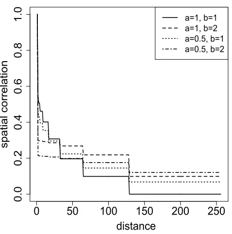
To better understand the covariance structure implied by Equation (12), Figure 1 presents
the posterior spatial correlation function for the log mean process at the finest resolution
level for different choices of the discount factor parameters. This correlation function was
computed at time t =T = 200 for data simulated from a model with 8 levels of resolution
in a one-dimensional spatial domain where each parent region has two children subregions.
The discount factor parameters were parameterized asδlj = 1−ae−bl. Hence, in this
specifi-cation the discount factor parameters decrease for higher resolution levels. Figure 1 presents
correlation functions for the four combinations of a= 1,0.5 and b = 1,2. Note that ae−b is
the magnitude of the change in the discount factors from one resolution level to the next.
A smaller value of b implies smaller values for the discount factors at higher resolutions.
That in turn leads to less smooth processes that are consistent, as shown in Figure 1, with
the spatial correlation function decreasing faster for b = 1 than for b = 2. Further, the
correlation function is a step function with step sizes that depend not only on the discount
factors but also on the number of resolution levels. More resolution levels would lead to an
ability to model more details and the spatial correlation function would have smaller steps.
Finally, even for a distance of 250 there is still substantial spatial correlation. Therefore, our
MSSTP model is able to accommodate spatial long range dependence.
the log mean process at the finest resolution level L may be written as
logµt+1,L,1:nL = A1:(L−1)
logµt1,1:n1 + log(ηt+1γ1:n1)
+
L−1
X
l=1
A(l+1):(L−1)
logωtl,1:nl+ log(φt+1,lj/St+1,lj) . (13)
In the right hand side of Equation (13), the first term shows the temporal evolution of the
temporal mean that is common to all subregions at the finest level that share the same
ancestor at the coarsest level. The second term shows the spatiotemporal evolution of
L−1
X
l=1
A(l+1):(L−1)logωtl,1:nl. (14)
Hence, PL−1
l=1 A(l+1):(L−1)logωtl,1:nl is the vector of dynamic spatiotemporal random effects
at the finest resolution level. Note that these spatiotemporal random effects at the finest
resolution level are impacted by the multiscale coefficients of ancestral nodes at all resolution
levels. Therefore, our MSSTP model implies at the finest resolution level a spatiotemporal
evolution composed of two components: a common temporal mean to all subregions that
share the same coarsest level ancestor; and dynamic spatiotemporal random effects that may
be affected by distinct dynamics at multiple resolution levels.
To better understand the spatiotemporal dependence structure, we compare our MSSTP
model to a widely used spatiotemporal model based on conditional autoregressions (STCAR)
for Poisson data. Specifically, in the STCAR model let ytj be the observed number of
counts at the finest resolution level at time t and subregion (L, j) and assume ytj|µtj ∼
P oisson(µtj), with log link logµtj =α0+aj+bt,j = 1, . . . , nL,t= 1, . . . , T. For this model,
the common mean follows a random walk bt = bt−1 +t, t ∼ N(0, W). In addition, the
spatial random effectsa1, . . . , anL follow a proper conditional autoregressive (CAR) structure
(Besag, 1974; Ferreira and de Oliveira, 2007) that assumes for the vector of spatial random
effects a = (a1, . . . , anL)
0 conditional distributions a
j|ai6=j ∼ N(¯aj,{(mj +d)τc}−1), where
¯
aj = (mj+d)−1Pi∈∂jai, ∂j is the set of neighbors of regionj,d is a propriety parameter as
is the number of neighbors of regionj. Note that in this STCAR model the spatial random
effects do not vary through time.
A particular case of our MSSTP model that has a structure similar to that of the STCAR
model is the degenerate case when all the discount factors for the multiscale coefficients
are equal to 1, that is, δlj = 1 for all l = 1, . . . , L −1, j = 1, . . . , nl. In that case, all
the multiscale coefficients are fixed through time, that is, ωtlj = ω0lj, t = 1, . . . , T, for
all l = 1, . . . , L −1, j = 1, . . . , nl. As a result, the spatiotemporal random effects given
in Equation (14) are fixed through time and play the role of the spatial random effects
a from the STCAR model. However, an important difference is that instead of a CAR
prior that assumes reasonably smooth spatial random effects, the spatial random effects in
our MSSTP model follow a multiscale spatial prior that may accommodate sharp transitions
among neighboring subregions. This multiscale spatial prior is similar to wavelet basis priors
that have been successfully used to account for spatial dependence in functional magnetic
resonance imaging (Flandin and Penny, 2007; Sanyal and Ferreira, 2012). Further, let us
assume that there is only one subregion at the coarsest level. Then, in this particular case
of our MSSTP model the log-mean at the coarsest level logµt1j corresponds to α0 +bt
in the STCAR model. Therefore, in the degenerate case when all the discount factors
for the spatiotemporal multiscale coefficients are equal to 1, our MSSTP model has a
log-mean spatiotemporal process that is the sum of a common temporal log-log-mean that follows
a random walk and spatial random effects that follow a multiscale spatial prior. Finally,
because the ωtlj’s allocate intensity in a multiscale manner to the subregions at the several
resolution levels, in the general case δlj ∈ (0,1) controls how much this intensity allocation
varies through time. Therefore, the dynamic spatiotemporal random effects in our MSSTP
model may incorporate distinct dynamics not only at the several resolution levels but also
at specific regions at each resolution level.
To the best of our knowledge, our MSSTP model does not nest other more traditional
has the capacity to perform much better than CAR-based spatiotemporal models. We think
that CAR-based models may be more adequate in cases when the underlying spatial random
effects are fairly smooth, and the smoothness is about the same in the entire region under
study. In contrast, our MSSTP will be more adequate when the spatial random effects are
not very smooth or in the case when the smoothness varies across the region of interest.
5
Applications
In this section we illustrate the usefulness of our MSSTP methodology with two
applica-tions. Section 5.1 examines mortality ratios in the state of Missouri and illustrates the case
when there is a known offset in the model, which in this application is the population size.
Section 5.2 considers tornado reports in the American Midwest and illustrates the case when
there is a regressor that at each time point is common to all regions. Finally, Section 5.3
presents a comparison of our MSSTP model for Poisson data to two competing models.
The first competing model assumes Poisson temporal evolution for each subregion at the
finest resolution level. The second competing model is the CAR-based model described in
Section 4.
In all applications presented in this section, we have used the same default prior
distri-butions. For the initial distributions λ01j|D0 and ω0lj|D0, we assume a0j = b0j = 0.01 and
c0lj = 0.011dlj, that imply vague prior information. In addition, for the priors for the
dis-count factors, we assume aγ =bγ = 1 and aδ =bδ = 1 which imply noninformative uniform
priors on the interval (0,1). Application of these default priors to a simulated data set (not
shown) leads our estimation methodology to recover the true values of the parameters. In
addition, we have performed a sensitivity study that has shown that results are not very
sensitivity to the choice of prior hyperparameters. Finally, we find that the default priors
5.1
Mortality in Missouri
This section presents an application of our MSSTP methodology to a data set of
mor-tality per county in the State of Missouri. The data set was downloaded from the website
www.dhss.mo.gov/DeathMICA/indexcounty.html of the Missouri Department of Health and
Senior Services. Specifically, here we consider the annual total number of deaths in the age
group from 45 to 64 years old from 1990 to 2009. The finest resolution level in this application
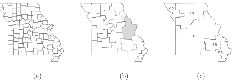
is the county level. Moreover, we assume the multiscale structure estimated by Ferreira et al.
(2011) for the state of Missouri. Specifically, we assume 3 levels of resolution (l = 1,2,3)
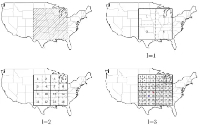
with a total of 115 counties at the finest level of resolution as presented in Figure 2. The
total number of deaths per county per year range from 0 to 1537, and several counties have
annual number of deaths less than 10. Because of these low counts, the use of a Gaussian
approximation would not be adequate. Thus, we apply here our MSSTP methodology for
Poisson data. In this application,ytLj is the number of deaths occurred in county j in yeart.
Moreover, we assumeytLj|λtLj ∼Poisson(λtLjetLj), where etLj is the population size divided
by 100,000 in county j in year t, and λtLj is the risk of death per 100,000 inhabitants in
county j in year t.
We advocate the analysis of the discount factors as a powerful way to identify regions with
spatiotemporal dynamics that warrant further investigation. For example, Figure 3 presents
the posterior densities for the discount factorsγj,δ1j, j = 1, . . . , n1, andδ2j, j = 1, . . . , n2. In
particular, Figure 3(a) presents the posterior densities for the discount factor parameters for
the risk at the coarsest level. Subregion (1,1) has the smallest discount factor and therefore
the least smooth temporal evolution with faster changes in the risk level through time. In
addition, Figure 3(b) presents the posterior densities for the discount factor parameters that
relate the coarsest level subregions with their descendants at the intermediate level. In
Figure 3(b), subregion (1,1) has again the smallest discount factor which indicates that its
descendants might have large changes in mortality risk through time. Furthermore, Figure
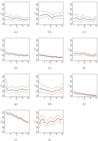
at the intermediate resolution level. In particular, in Panel (c) the left-most posterior density
is forδ2,6indicating that the descendants of subregion (2,6), that is, counties within the Saint
Louis metropolitan area, have the most temporal change in relative importance. To further
investigate this issue, Figure 4 presents the estimated risk per 100,000 inhabitants for the
45 to 64 years old age group for counties within the Saint Louis metropolitan area. Several
counties have decreasing risk and, in particular, panel (j) shows a substantial and steady
rate of decrease in risk through time for the City of Saint Louis.
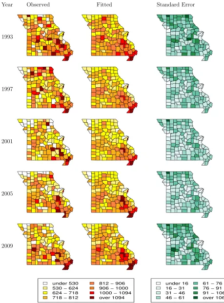
Finally, Figure 5 presents maps of estimated risk per county of the State of MIssouri
per 100,000 inhabitants for the 45 to 64 years old age group. Specifically, Figure 5 presents
the maps of observed standardized mortality ratio (left panels), posterior medians (central
panels), and standard errors (right panels) for years 1993, 1997, 2001, 2005, and 2009. As
intuitively expected, the standard errors decrease with county population size. Moreover,
because the observations have Poisson distribution, the standard errors increase with county
mean risk level. In addition, the standard errors are mostly below 100, and typically around
50. Hence, the use of color-coded intervals of length 94 for the observed and fitted maps
allows for meaningful interpretation.
Analysis of the fitted maps shows that our MSSTP methodology is able to provide fitted
maps much smoother than the observed maps. At the same time, our methodology respects
sharp transitions between neighboring regions. For example, the fitted maps preserve the
much higher risk of the City of Saint Louis when compared with Saint Louis County. From
an epidemiological perspective, the fitted maps show that the northern counties have lower
death rates than the southern counties. In particular, several counties in the southeast part
of Missouri have persistently high death rates.
5.2
Tornadoes in the American Midwest
This section presents a MSSTP analysis of annual tornado report data from 1953 to 2010
F1 (weaker) to F5 (stronger). Here we consider the more intense tornadoes from F3 to
F5. For each tornado we consider only the year and the location of the first touchdown.
The region of interest is the tornado alley which is the area with the highest incidence of
tornadoes in the United States. Specifically, here we consider the rectangle region defined by
the north-most boundary of South Dakota, the west-most boundary of South Dakota, the
south-most boundary of Mississippi and the east-most boundary of Michigan, as presented in
Figure 6. Furthermore, we consider three spatial resolution levels: a coarse resolution with
4 subregions, an intermediate resolution with 16 subregions, and a fine resolution with 64
subregions. Thus, ytLj is the number of tornado touchdowns in year t in the j-th subregion
at the finest resolution level.
To account for the relationship between tornado occurrence and the El Ni˜no and La
Ni˜na phenomena (Monfredo, 1999; Wikle and Anderson, 2003), we assume ytLj|λtLj, βLj ∼
Poisson(λtLjetLj), where etLj = exp(xtβLj), xt is the average Southern Oscillation Index
(SOI) for the months of March, April and May in year t, and βLj = βA1(L,j), with A1(L, j)
being the ancestor at resolution level l = 1 of subregion (L, j). That is, we assume that the
El Ni˜no and La Ni˜na phenomena may have a different impact on each of the four coarse level
regions. For simplicity of notation, we denote βj = β1j, j = 1, . . . ,4. Figure 7(a) presents
the posterior densities for βj, j = 1, . . . ,4, which indicate that increases in the SOI are
related to increases in the risk of tornado in subregions (1,2), (1,3), and (1,4) at the coarsest
resolution level. In addition, risk of tornado in subregion (1,1) does not seem to be related to
the SOI. Thus, its northern position and proximity to the Rocky Mountains seem to isolate
subregion (1,1) from the influence of the El Ni˜no and La Ni˜na phenomena. Finally, Figure
7(b) presents the posterior densities ofγj,j = 1, . . . ,4. These posterior densities are located
below 0.6 which indicate that, after accounting for the SOI, there are fast temporal changes
in the risk of tornado for all four coarse level regions.
Figure 7(c) presents the posterior densities of δ1j, j = 1, . . . ,4, which indicate that the
through time. This suggests that we should investigate in more detail the descendants of
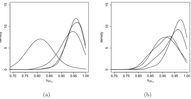
subregions (1,3) and (1,4). Figure 8(a) presents the posterior densities for δ2j for j ∈ D1,3,
whereas Figure 8(b) presents the posterior densities for δ2j for j ∈ D1,4. On Panel (a), the
notably smaller discount factor corresponds to subregion (2,10); specifically, the posterior
mean of δ2,10 is equal to 0.81. This indicates that the spatiotemporal multiscale coefficient
ωt,2,10 that relates subregion (2,10) to its descendants changes substantially through time
and should be investigated in more detail.
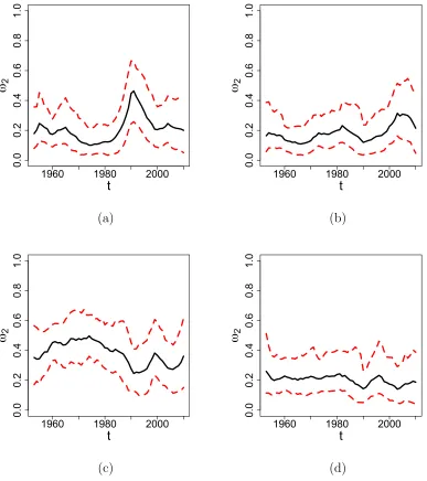
Figure 9 shows the time series plot of posterior median (solid line) and 95% credible
interval (dashed line) for each element of ωt2,10. Each element of ωt2,10 corresponds to one
descendant of subregion (2,10). These descendents are (3,37) (panel a), (3,38) (panel b),
(3,39) (panel c) and (3,40) (panel d). For reference, note that if the relative risk was the
same for all four descendants then the spatiotemporal multiscale coefficient would have all
elements equal to 0.25. Thus, the posterior probability that an element of the spatiotemporal
multiscale coefficient is larger than 0.25 provides a measure of whether the corresponding
region has relative risk higher or lower than its siblings. Let us call this probability the
exceedance probability. As a consequence, two features are worth mention: the first feature
is that the exceedance probability for subregion (3,39) is above 0.9 from 1950 to 1980. That
is, during that period subregion (3,39) had substantially higher risk than its siblings. The
second feature is that the relative risks between subregions (3,37), (3,38), (3,39), and (3,40)
have been changing substantially since 1980. This may indicate that subregion (2,10) may
be particularly susceptible to the effects of climate change.
Additional evidence of the importance of subregion (2,10) for studies of climate change
is given by considering the number of F5 tornadoes. F5 are the strongest tornadoes and are
much less likely to be underreported. Here we consider a comparison of the period from 1950
to 2010 (used in our multiscale analysis) to the period from 2011 to 2014 (not included in
our multiscale analysis). During the period from 1950 to 2010 there were 52 F5 tornadoes in
during the period from 2011 to 2014 there were 7 F5 tornadoes in the United States and 3 of
those, or 42.8%, occurred in subregion (2,10). Hence, Earth atmospheric variables conducive
to the formation of tornadoes seem to be changing substantially within subregion (2,10).
Therefore, a detailed future study of subregion (2,10) may shed light on what are these
Earth atmospheric variables and how they are being impacted by global warming.
While one of the three tornadoes that occurred in subregion (2,10) from 2011 to 2014 hit
a less populated area, the other two tornadoes hit more densely populated areas. Specifically,
these two tornadoes hit Joplin, Missouri, in 2011, and Moore, Oklahoma, in 2013, causing
estimated losses of about 4.8 billion dollars and 182 deaths. For reference, the lower right
panel of Figure 6 shows the locations of Joplin (red dot) and Moore (blue dot). Therefore,
a detailed future study of subregion (2,10) may not only help identify important Earth
atmospheric variables impacted by global warming, but may also help improve tornado alert
systems to reduce property and human life losses.
5.3
Model comparison
This section presents a comparison of our MSSTP model to two competing models. First, to
access the ability of our multiscale spatiotemporal framework to borrow strength spatially,
we compare our model to a model that assumes that each finest level subregion has its
own independent temporal evolution (ITE). Second, to access our framework’s ability to
incorporate spatiotemporal dynamics, we compare our model to the STCAR model described
in Section 4. We perform these model comparisons using conditional Bayes factors (e.g., see
Ghosh et al., 2006) and the deviance information criterion (DIC) (Spiegelhalter et al., 2002)
for both Missouri and tornado data sets.
We have implemented the conditional Bayes factor for both models following the
simulation-based approach proposed by Vivar and Ferreira (2009). This approach uses
the data observed at the first t∗ times points as a training sample. Specifically, let
q given the data up to time t. Then, the one-step-ahead predictive density is
pq(yt+1|Dt) =
Z
pq(yt+1|µt+1,L,1:nL,γ,δ)pq(µt+1,L,1:nL|µt,L,1:nL,γ,δ,Dt)
×pq(µ1:t,L,1:nL,γ,δ|Dt)dµ1:(t+1),L,1:nLdγdδ.
The posterior simulation algorithms presented in Section 3 can be easily used to estimate the
above one-step-ahead predictive density. Then, the joint predictive density of yt∗+1, . . . ,yT
can be computed as pq(yt∗+1, . . . , yT|Dt∗) =QT
t=t∗+1pq(yt|Dt−1) (e.g., see p. 135 Prado and
West, 2010) Finally, the conditional Bayes factor of model q1 against model q2 is equal to
Bq1,q2 =
pq1(yt∗+1, . . . ,yT|Dt∗)
pq2(yt∗+1, . . . ,yT|Dt∗)
.
Therefore, the conditional Bayes factor uses the one-step-ahead predictive densities and,
thus, effectively compares the predictive performance of the competing models.
First, we compare our MSSTP model to an ITE model that assumes that each finest level
subregion has its own temporal evolution according to the Poisson state-space model given
by the observational equation (1) and the beta evolution equation (4). Here we have used
t∗ = 10 for the Missouri data set and t∗ = 18 for the tornado report data set. These values
for t∗ provide stable analyses and allow for each data set many time points to be used in
the model comparison. For the data set on mortality ratio in Missouri, the logarithm of the
conditional Bayes factor of our MSSTP model against the ITE model is equal to 39.24 which
provides strong evidence in favor of our MSSTP model. Further, the DIC of our MSSTP
model is 15,120.23 whereas the DIC of the ITE model is 15,145.10. Hence, the DIC agrees
with the conditional Bayes factor and chooses our MSSTP model for the Missouri data set.
For the tornado report data, the logarithm of the conditional Bayes factor is equal to 326.21,
again providing strong evidence in favor of our MSSTP model. In addition, the DIC of our
MSSTP model is 7,385.67 and the DIC of the ITE model is 7,690.95. Once again, the DIC
agrees with the conditional Bayes factor and chooses our MSSTP model for the tornado data
set. Hence, in both applications the conditional Bayes factor and the DIC provide strong
that does not use spatial information, this result implies that our MSSTP model superiority
arises from its ability to borrow strength spatially.
Second, we compare our MSSTP model to the STCAR model considered in Section 4 that
assumes Poisson distribution for the observations, and a logarithm link function that connects
the mean of each observation to a sum of a temporal trend and spatial random effects. We
assume the priors φ∼ Beta(1,1), p(α0)∝ 1,τc ∼Ga(0.5,0.0005), b0 ∼N(0,2000), logd ∼
Ga(1,1),W ∼Ga(0.5,0.0005). As in the previous model comparison, in the computation of
the conditional Bayes factor we have used t∗ = 10 for the Missouri data set and t∗ = 18 for
the tornado report data set. The logarithm of the conditional Bayes factor of our MSSTP
model against the STCAR model is equal to 10.28 for the data set on mortality ratio in
Missouri, and is equal to 84.27 for the tornado report data set. Meanwhile, the DICs for the
STCAR model are 15,307.37 for the Missouri data set and 7,874.39 for the tornado data set.
Therefore, in both applications the conditional Bayes factor and the DIC provide evidence
of the superiority of our MSSTP model to incorporate spatiotemporal dynamics.
A fair question is whether or not our MSSTP model is identifiable. Or in other words,
are the conditional Bayes factor and the DIC able to correctly distinguish amongst the three
models considered above. To answer this question, we have performed a simulation study
where we have simulated 10 data sets from each of the three models. In this simulation
study, we have used the multiscale structure of the state of Missouri as depicted in Figure
2 in which n0 = 5, n1 = 22 and n2 = 115. To simulate the data sets from our MSSTP
model we have used γ = (0.98,0.98,0.95,0.95,0.98), δ1 = (0.98,0.98,0.98,0.95,0.95) and
δ2 = 0.981n1. To simulate the data sets from the ITE model, the discount factors for the 115
counties were simulated independently from a uniform distribution on the interval (0.4,1).
To simulate data from the STCAR model, we have assumedτc= 1,d = 1, andW = 0.1. We
assess the performance of the conditional Bayes factor and the DIC in terms of the success
rate in choosing the correct model. For the three models, the DIC selected the correct model