Full Terms & Conditions of access and use can be found at
http://www.tandfonline.com/action/journalInformation?journalCode=lsta20
Download by: [Lancaster University] Date: 06 July 2017, At: 05:10
Communications in Statistics - Theory and Methods
ISSN: 0361-0926 (Print) 1532-415X (Online) Journal homepage: http://www.tandfonline.com/loi/lsta20
Note on Posterior Inference for the Bingham
Distribution
Mike G. Tsionas
To cite this article: Mike G. Tsionas (2017): Note on Posterior Inference for the Bingham Distribution, Communications in Statistics - Theory and Methods, DOI: 10.1080/03610926.2017.1346805
To link to this article: http://dx.doi.org/10.1080/03610926.2017.1346805
Accepted author version posted online: 30 Jun 2017.
Submit your article to this journal
Article views: 6
View related articles
Note on Posterior Inference for the Bingham Distribution
Mike G. Tsionas
∗14th June 2017
Abstract
The properties of high-dimensional Bingham distributions have been studied by Kume and Walker (2014). Fallaize and
Kypraios (2016) propose Bayesian inference for the Bingham distribution and they use developments in Bayesian computation
for distributions with doubly intractable normalising constants (Møller et al. 2006; Murray et al. 2006). However, they rely
heavily on two Metropolis updates that they need to tune. In this paper we propose instead model selection with the marginal
likelihood.
Key words: Bingham distribution; Bayesian; Markov Chain Monte Carlo; marginal likelihood.
Acknowledgements: The author is grateful to an anonymous reviewer for helpful comments on an earlier version.
∗Lancaster University Management School, LA1 4YK, U.K. & Athens University of Economics and Business, Greece, m.tsionas@lancaster.ac.uk
1
ACCEPTED MANUSCRIPT
1
Introduction
The properties of high-dimensional Bingham distributions have been studied by Kume and Walker (2014). Bee, Benedetti and
Espa (2017) have considered approximate maximum likelihood estimation of the Bingham distribution. Fallaize and Kypraios
(2016) propose Bayesian inference for the Bingham distribution and they use developments in Bayesian computation for
dis-tributions with doubly intractable normalising constants (Møller et al. 2006; Murray et al. 2006). However, they rely heavily
on two Metropolis updates that they need to tune. In this paper we rely on Walker (2014) but we avoid his reversible-jump
MCMC via model selection with the marginal likelihood. Here, we avoid altogether computational inefficiencies introduced by
reversible-jump MCMC. It is known that this type of MCMC requires considerable tuning and contributes to higher
autocorrel-ation functions and, therefore, lower efficiency in MCMC. As this step can be avoided, MCMC can, in principle, be made more
efficient. Walker (2011) proposed an infinite mixture along the lines of Godsill (2001). Here, we propose to consider different
values for the number of mixing components and choose the one that maximizes the marginal likelihood which, for fixed number
of mixing components, can be obtained using the method of Perrakis, Ntzoufras and Tsionas (2014). Walker (2014) used the
ideas above but resorted to reversible jump MCMC (Green, 1995), a fact that was shown that can be bypassed in Fallaize and
Kypraios (2016). The method we propose here, avoids both the use of reversible jump MCMC as in Walker (2013) and also the
Metropolis updates in Fallaize and Kypraios (2016).
2
Methods
2.1
Fixed
A
The Bingham distribution is
p(x;A) = 1
c(A)exp(−x
0Ax), x∈ <q, x0x= 1, (1)
wherec(A) is an intractable integration constant andAis a q×q symmetric matrix. The standard form of the distribution is:
p(x; Λ) = 1 c(Λ)exp
(
−
q−1
X
i=1 λix2i
)
, (2)
with respect to a uniform measure on the sphere and
c(Λ) = ˆ
Sq−1 exp
(
−
q−1
X
i=1 λix2i
)
dSq−1(x), (3)
whereSq−1 is the unit sphere in<q, andΛ =diag(λ
1, ..., λq) under the identifiability constraint
λ1≥...≥λq−1≥λq = 0. (4)
We need these constraints as the density does not change if we add a positive constant to theλis, see Bingham (1974).
2
ACCEPTED MANUSCRIPT
IfA=VΛV0 where V is orthonormal, if X follows a Bingham distribution with densityp(x;A) then Y =V X follows a
Bingham distribution with densityp(x; Λ), see Kume and Walker (2006). The maximum likelihood estimator ofV is the matrix
of eigenvectors ofPT
t=1xtx0t.
The joint density from a random sampleX={xt;t= 1, ..., T} gives rise to the likelihood:
L(Λ;X) =c(Λ)−Texp
(
−
q−1
X
i=1 λiQi
)
, (5)
whereQi=P T t=1x
2
ti. Given a prior, sayp(Λ) we have the posterior:
p(Λ|X)∝c(Λ)−Texp
(
−
q−1
X
i=1 λiQi
)
p(Λ). (6)
It is possible to introduce an auxiliary variablev so that
p(Λ, v|X)∝vT−1exp{−c(Λ)v}exp
(
−
q−1
X
i=1 λiQi
)
p(Λ). (7)
However, sincec(Λ) is intractable this is not much help. Following Walker (2011) we can introduce variables (k, s1, ..., sk)
to have:
p(Λ, v, k, s(k)|X)∝v
T+k−1exp(−v) k! exp ( − q−1 X i=1 λiQi
) k
Y
j=1
[1−p(s˜ j; Λ)]p(Λ), (8)
where ˜p(s; Λ) = expn−Pq−1
j=1s2jλj
o
, s(k)≡(s
1, ..., sk)∈(0,1), for all k. Further latent variables u1, ..., uk can be introduced and they contribute a term:
k
Y
j=1
1(uj <1−p(s˜ j; Λ)).
The conditional posterior ofv is gamma(T +k,1). The conditional posterior foruj is uniform in (0, 1−p(s˜ j; Λ)). The
conditional posterior forsj is uniform in{s∈(0,1) : ˜p(s; Λ)<1−uj}. If we integrate outv we get:
p(Λ, k, s(k)|X)∝
T+k−1
k k Y j=1
[1−p(s˜ j; Λ)] exp
(
−
q−1
X
i=1 λiQi
)
p(Λ). (9)
The conditional posterior for Λ is:
p(Λ|k, s(k), X)∝exp
(
−
q−1
X
i=1 λiQi
)
p(Λ)1(θ∈A), (10)
whereA={θ: p(sj; Λ)<1−uj, ∀j= 1, ..., k}.
Walker (2011) proposed an infinite mixture for k, s(k), u
along the lines of Godsill (2001). Here, we propose to consider
values of k= 1, ..., k and choose the one that maximizes the marginal likelihood which, for fixedk, can be obtained from (9)
3
ACCEPTED MANUSCRIPT
using the method of Perrakis, Ntzoufras and Tsionas (2014). Walker (2014) used the ideas above but resorted to reversible jump
MCMC (Green, 1995), a fact that was shown that can be bypassed in Fallaize and Kypraios (2016). The method we propose
here, avoids both the use of reversible jump MCMC as in Walker (2013) and also the Metropolis updates in Fallaize and Kypraios
(2016).
2.2
Posterior inference for
A
The conditional posterior ofA, if we assign normal priorsN(0, h2) to its elements is given by:
p(A|.)∝
expn−PT
t=1y 0
tAyt−21h2a0a
o
c(A)n =
expn−detAQ− 1 2h2a0a
o
c(A)n , (11)
where a is the vector of distinct elements ofA and Q =PT
t=1yty0t. We can use the same “trick” as in (7) and introduce an auxiliary variablev so that:
p(A|·)∝vT−1exp
−AQ− 1
2h2a
0a−c(A)v, (12)
but sincec(A) is unknown this is not very helpful. However, we can proceed by introducing additional latent variablesK and
S(k), as we did in (8). We avoid, again, the infinite mixture construction and reversible-jump MCMC by using model selection
forKvia the marginal likelihood. It can be shown that each different element ofAin the final conditional posterior distribution
follows a normal distribution subject to constraints similar to those that we provided previously for Λ.
3
Applications
We apply our techniques to two artificial data sets as described in Fallaize and Kypraios (2016). For both sets we use 15,000
iterations the first 5,000 of which are discarded to mitigate start up effects.
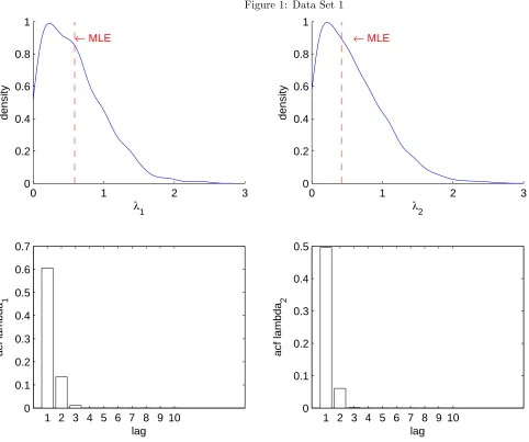
DATA SET 1. We consider a sample ofn= 100 unit vectors which result approximately in the pair of sufficient statistics
(τ1, τ2) = (0.30, 0.32) where τi = P n t=1y
2
ti. We assign independent exponential prior distributions with mean 100 to the parametersλ1andλ2.Mardia and Zemroch (1977) report maximum likelihood estimates of 0.588 and 0.421.
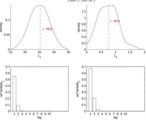
DATA SET 2. We consider an artificial dataset of 100 vectors which result approximately in the pair of sufficient statistics
(τ1, τ2) = (0.02, 0.40)for which the maximum likelihood estimates are 25.31 and 0.762 as reported in Mardia and Zemroch (1977).
We use the same priors as in data set 1.
Marginal posterior densities of λ1and λ2 and their autocorrelation functions from MCMC are reported in Figure 1 for
data set 1 and in Figure 2 for data set 2. The marginal posteriors are visually very close to the ones reported in Fallaize and
Kypraios (2016) but MCMC autocorrelations are substantially smaller.
In Figure 3 we present normalized marginal likelihoods for selection ofkin the two data sets (we normalize the marginal
likelijhood to 1 whenk= 1). In both cases the marginal likelihood favoursk=20.
4
ACCEPTED MANUSCRIPT
Figure 1: Data Set 1
0 1 2 3
0 0.2 0.4 0.6 0.8 1
← MLE
λ1
density
0 1 2 3
0 0.2 0.4 0.6 0.8 1 λ2 density
← MLE
1 2 3 4 5 6 7 8 9 10 0 0.1 0.2 0.3 0.4 0.5 0.6 0.7 lag acf lambda 1
1 2 3 4 5 6 7 8 9 10 0 0.1 0.2 0.3 0.4 0.5 lag acf lambda 2
DATA SET 3. To illustrate inference for a general matrixAwe use the data of Bingham (1974) as in Fallaize and Kypraios
(2016). The data consist ofn= 150 measurements on the c-axis of calcite grains from the Taconic Mountains of New York state.
We useh=10. For the diagonal components of Λ, Fallaize and Kypraios (2016) obtain posterior median values λ1 = 3.631 and
λ2 = 1.963. We obtain 3.60 and 1.942 respectively. ForV, the orthonormal component matrix of A, our posterior means are:
V =
0.1751 −0.4423 0.8812
0.1375 0.8932 0.4251
−0.9681 0.0463 0.2195
,
which in in broad agreement with the results in Fallaize and Kypraios (2016).
5
ACCEPTED MANUSCRIPT
Figure 2: Data Set 2
15 20 25 30 35
0 0.05 0.1
← MLE
λ1
density
0 0.5 1 1.5 2
0 0.2 0.4 0.6 0.8 1 1.2
λ2
density
← MLE
1 2 3 4 5 6 7 8 9 10 0
0.1 0.2 0.3 0.4 0.5 0.6 0.7
lag
acf lambda
1
1 2 3 4 5 6 7 8 9 10 0
0.1 0.2 0.3 0.4 0.5 0.6 0.7
lag
acf lambda
2
6
ACCEPTED MANUSCRIPT
Figure 3: Normalized marginal likelihood to selectk
0 10 20 30 40 50 60
0 10 20 30 40 50 60 70
k
normalized marginal likelihood
Data Set 1 Data Set 2
7
ACCEPTED MANUSCRIPT
Table 1: Statistics q acf(10) acf(50) RNE
5 0.215 0.814
0.101 0.717
0.516 0.215 10 0.222
0.821
0.115 0.789
0.603 0.188 15 0.237
0.832
0.120 0.753
0.682 0.142 20 0.255
0.891
0.129 0.801
0.727 0.110
Notes: Figures in italics denote results from the Walker (2014) approach. We report median statistics taken across the 5,000 different random samples that we consider for each value ofq. We report the median MCMC autocorrelation at lag 10 (denoted acf(10)), the median MCMC autocorrelation at lag 50 (denoted acf(50)), and relative numerical efficiency (RNE), see Geweke (1992). A relative numerical efficiency close to unity indicates random (i.i.d) sampling. MCMC is implemented using 15,000 iterations the first 5,000 of which are discarded.
4
Comparison in higher dimensions
To compare the new techniques with the one proposed in Walker (2014) we fix the sample size atn= 150, in broad agreement
with the applications in the previous section and we consider larger dimensional spheres, that is larger values ofq. For each
value ofq, we assign independent exponential prior distributions with mean 100 to the parametersλj. We generate the sufficient
statistics from a uniform distribution in the interval [50, 104]. The true values of the diagonal components of Λ, are generated
from uniform distributions in [1,5]. The elements ofV, the orthonormal component matrix ofA, are generated from standard
normal distributions. Finally, random samples from the Bingham distribution are generated according to the procedure of Kent
et al. (2004). For each value ofq, we generate 5,000 different random samples of sizenfrom the Bingham distribution.
In Table 1, we report median statistics taken across the 5,000 different random samples that we consider for each value
ofq. We report the median MCMC autocorrelation at lag 10 (denoted acf(10)), the median MCMC autocorrelation at lag 50
(denoted acf(50)), and relative numerical efficiency (RNE), see Geweke (1992). A relative numerical efficiency close to unity
indicates random (i.i.d) sampling. Our autocorrelations at lags 10 and 50 are substantially smaller compared to Walker (2014)
and RNE increases as the dimensionality q increases. In contract, Walker’s (2014) RNE decreases. This is evidence that the
performance of the new approach is much better and, in large dimensional spheres, is not extremely far from delivering i.i.d.
samples from the posterior.
References
Bee, M., R. Benedetti and G. Espa (2017). Approximate maximum likelihood estimation of the Bingham distribution.
Compu-tational Statistics and Data Analysis 108, 84-96.
Bingham, C. (1974). An antipodally symmetric distribution on the sphere. Annals of Statistics 2, 1201–1225.
Fallaize, C.J., Kypraios, T. (2016). Exact Bayesian inference for the Bingham distribution. Statistics and Computing 26,
349–360.
Geweke, J. (1992), Evaluating the Accuracy of Sampling-Based Approaches to the Calculation of Posterior Moments. In
Bayesian Statistics 4 (eds. J.M. Bernardo, J. Berger, A.P. Dawid and A.F.M. Smith), Oxford: Oxford University Press, 169-193.
8
ACCEPTED MANUSCRIPT
Godsill, S. J. (2001). On the relationship between Markov chain Monte Carlo methods for model uncertainty. Journal of
Computational and Graphical Statistic 10:230–248.
Green, P. J. (1995). Reversible jump Markov chain Monte Carlo computation and Bayesian model determination.
Bio-metrika 82, 711–732.
Kent, J.T., Constable, P.D.L. & Er, F. (2004). Simulation for the complex Bingham distribution. Statistics and Computing
14, 53–57
Kume, A., Walker, S.G. (2006). Sampling from compositional and directional distributions. Statistics 16, 261–265.
Kume, A., Walker, S.G. (2014). On the Bingham distribution with large dimension. Journal of Multivariate Analysis 124,
345–352.
Mardia,K.V., Zemroch, P.J.: Table of maximum likelihood estimates for the Bingham distribution. Statist. Comput.
Simul. 6, 29–34 (1977)
Møller, J., Pettitt, A.N., Reeves, R., Berthelsen, K.K. (2006). An efficient Markov chain Monte Carlo method for
distributions with intractable normalising constants. Biometrika 93(2), 451–458.
Murray, I., Ghahramani, Z., MacKay, D.J.C. (2006). MCMC for doubly intractable distributions. In Proceedings of the
22nd annual conference on uncertainty in artificial intelligence (UAI-06), pages 359– 366. AUAI Press.
Perrakis, K., Ntzoufras, I. and Tsionas, E. (2014). On the use of marginal posteriors in marginal likelihood estimation via
importance-sampling. Computational Statistics and Data Analysis, 77, 54-69.
Walker, S.G. (2012). Posterior sampling when the normalizing constant is unknown. Communications in Statistics
-Simulation and Computation, 40:5, 784-792.
Walker, S.G. (2014). Bayesian estimation of the Bingham distribution. Brazilian Journal of Probability and Statistics,
28(1), 61–72.
9