Proteus:Network aware Web Browsing on Heterogeneous Mobile Systems

Network-aware Web Browsing on Heterogeneous Mobile

Systems

ABSTRACT

Web browsing is an important application domain. However, it imposes a significant burden on battery-powered mobile devices. While heterogeneous multi-cores offer the potential for energy-efficient mobile web browsing, existing web browsers fail to exploit the heterogeneous hardware because they are not tuned for typical networking environments and web workloads, and there are few existing efforts that try to lower the energy consumption of web browsing for heterogeneous mobile platforms.

Our work introduces a better way to optimize web browsing on heterogeneous mobile devices. We achieve this by developing a machine learning based approach to predict which of the CPU cores to use and the operating frequencies of CPU and GPU. We do so by first learning,offline, a set of predictive models for a range of networking environments. We then choose a learnt model at runtime to predict the optimal processor configuration. The pre-diction is based on the web content, the network status and the optimization goal. We evaluate our approach by applying it to the open-source Chromium browser and testing it on two represen-tative heterogeneous mobile multi-cores platforms. We apply our approach to the top 1000 popular websites across seven typical networking environments. Our approach achieves over 80% of best available performance. We obtain, on average, over 17% (up to 63%), 31% (up to 88%), and 30% (up to 91%) improvement respectively for load time, energy consumption and the energy delay product, when compared to two state-of-the-art mobile web browsing schedulers.

CCS CONCEPTS

•Computer systems organization→Embedded software; • Computing methodologies→Parallel computing methodologies;

KEYWORDS

Mobile web browsing, Energy optimization, Heterogenous multi-cores

ACM Reference Format:

. 2018. Network-aware Web Browsing on Heterogeneous Mobile Systems. In

Proceedings of CoNEXT (CoNEXT ’18).ACM, New York, NY, USA, 14 pages. https://doi.org/10.1145/nnnnnnn.nnnnnnn

Permission to make digital or hard copies of all or part of this work for personal or classroom use is granted without fee provided that copies are not made or distributed for profit or commercial advantage and that copies bear this notice and the full citation on the first page. Copyrights for components of this work owned by others than ACM must be honored. Abstracting with credit is permitted. To copy otherwise, or republish, to post on servers or to redistribute to lists, requires prior specific permission and/or a fee. Request permissions from [email protected].

CoNEXT ’18, Heraklion, Greece, 2018 © 2018 Association for Computing Machinery. ACM ISBN 978-x-xxxx-xxxx-x/YY/MM. . . $15.00 https://doi.org/10.1145/nnnnnnn.nnnnnnn

1

INTRODUCTION

Web is a major information portal on mobile devices [28]. However, web browsing is poorly optimized and continues to consume a significant portion of battery power on mobile devices [15, 17, 46]. Heterogeneous multi-cores, such as the ARM big.LITTLE architec-ture [1], offer a new way for energy-efficient mobile computing. Moreover, today’s mobile devices are also equipped with powerful GPUs. Thus, hardware acceleration of web browsing using mo-bile GPUs alongside the central processing unit is beginning to be possible.

These platforms integrate multiple processor cores on the same system, where each processor is tuned for a certain class of work-loads to meet a variety of user requirements. However, it is currently challenging to unlock the potential of heterogeneous multi-cores, because doing so requires the web browsers to know e.g., which processor core to use and at what frequency the core should operate. Current mobile web browsers rely on the operating system to exploit the heterogeneous cores. Since the operating system has little knowledge of the web workload and how does the network affect web rendering, the decision made by the operating system is often sub-optimal. This leads to poor energy efficiency [54], drain-ing the battery faster than necessary and irritatdrain-ing mobile users. In this work, we ask the research question: “What advantages can a scheduler take when it knows the web workload and the impact of the networking environment?". In answer, we develop new tech-niques to exploit knowledge of the computing environment and web workloads to make better use of the underlying hardware.

In this work, we are interested at choosing the best processor (CPU and GPU) configuration for a given web workload under a spe-cific networking environment. We focus on processor scheduling because processors are the major energy consumer on mobile de-vices and their power consumption has continuously increased on recent processor generations [23]. Rather than letting the operating system make all the scheduling decisions by passively observing the system’s load, our work enables the browser to actively par-ticipate in decision making. Specifically, we want the browser to decide which heterogeneous CPU core and the optimal CPU and GPU frequencies to use to run the rendering engine and painting process. We show that a good decision must be based on the web content, the optimization goal, and how the network affects the rendering process.

web content

Parsing _ResolutionStyle Render _Layout Painting

Style Rules

Training webpages

Profiling runs

Feature extraction

optimal proc. config.

feature values

L

ea

rn

in

g

A

lg

or

ith

m

Predictive Model extractionFeature

optimal proc. config.

webpage feature values

L

ea

rn

in

g

A

lg

or

ith

m

Predictor Training

webpages Profiling

runs

features values

Browser Extension

processor config.

Network Monitor

delay&bandwidth

scheduling

web contents

Predictive Model <html>

... </html>

a b

Web Server

Web

Server Screen

DOM Tree

Render Tree

Fetching

Rendering Engine

Graphic Data

Painting Process

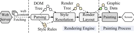
Figure 1: The processing procedure of Chromium.

Such an approach avoids the pitfalls of using a hard-wired heuris-tics that require human modification every time the computing environment or hardware changes.

We have implemented our techniques in the open-sourced Google Chromium web browser. We evaluate our approach by applying it to the top 1,000 popular websites ranked byalexa.com[4], including Facebook, Amazon, CNN, etc. We test our techniques under seven typical cellular and WiFi network settings. We compare our ap-proach against two state-of-art web browser schedulers [40, 55] on two distinct heterogeneous mobile platforms: Odroid XU3 and Jet-son TX2. We consider three metrics: load time, energy consumption and the energy delay product (see Section 2.3). Experimental results show that our approach consistently outperforms state-of-the arts across evaluation metrics and platforms.

The key contribution of this paper is a novel machine learning based web rendering scheduler that can leverage knowledge of the network and webpages to optimize mobile web browsing. Our results show that significant energy efficiency for heterogeneous mobile web browsing can be achieved if the scheduler is aware of the networking environment and the web workload. Our techniques are generally applicable, as they are useful for not only web browsers but also a large number of mobile apps that are underpinned by web rendering techniques [16].

2

BACKGROUND AND MOTIVATION

2.1

Web Processing

Our prototype system1is built upon Chromium [6], an open source version of the popular Google Chrome web browser.

Figure 1 illustrates how Chromium handles a webpage. The web contents, e.g., HTML pages, CSS styles, Javascripts and multimedia contents, are fetched by a network process. The downloaded content is processed by therendering engine process. The rendering results are passed to thepainting processto generate visualization data in the GPU buffer to display to the user. This pipeline of rendering and screen painting is calledcontent painting. To render the web content, the rendering engine constructs a Document Object Model (DOM) tree where each node of the tree represents an individual HTML tag like<body>or<p>. CSS style rules that describe how the web contents should be presented are also parsed by the rendering engine to build the style rules. After parsing, styling information and theDOMtree are combined to build a render tree which is then used to compute the layout of each visible element. To paint the web content, the painting process reads the rendered graphic data and outputs the rendered contents at the pixel level to the screen.

1_{Code is available at: [url redacted for double-blind review].}

Table 1: The best-performing existing governor

Load time Energy EDP

CPU GPU CPU GPU CPU GPU

Regular 3G Perf. Default powersave Static powersave Booster

Regular 4G Perf. Default conservative Static Inter. Booster

WiFi Inter. Default ondemand Booster Inter. Booster

2.2

Problem Scope

Our work focuses on scheduling the time-consumingrenderingand

paintingprocesses on heterogeneous mobile multi-cores. The goal is to develop a portable approach to automatically determine, for a given webpage in a networking environment, the optimal processor configuration. A processor configuration consists of three param-eters: (1) which heterogeneous CPU to use to run the rendering process, (2) what are the clock frequencies for the heterogeneous CPUs, and (3) the GPU frequency for running the painting process.

2.3

Motivation

Consider a scenario for browsing fourBBCnews pages, starting from the home page ofnews.bbc.co.uk. In the example, we assume that the user is an average reader who reads 280 words per minute [30] and would click to the next page after finishing reading the current one. Our evaluation device in this experiment is Odroid XU3 (see Section 5.1), an ARM big.LITTLE mobile platform with a Cortex-A15 (big) and a Cortex-A7 (little) CPUs, and a Mali-T628 GPU. Networking Environments.We consider three typical network-ing environments (see Section 4.1 for more details): Regular 3G, Regular 4G and WiFi. To ensure reproducible results, web requests and responses are deterministically replayed by the client and a web server respectively. The web server simulates the download speed and latency of a network setting, and we record and determinis-tically replay the user interaction trace for each testing scenario. More details of our experimental setup can be found at Section 5.1. Oracle Performance.We schedule the Chromium rendering en-gine (i.e.,CrRendererMain) to run on either the big or the little CPU core under different clock frequencies. We also run the GPU painting process (i.e.,Chrome_InProcGpuThread) under different GPU frequencies. We record the best processor configuration per test case per optimization target. We refer this best-found configu-ration as theoraclebecause it is the best performance we can get via processor frequency scaling and task mapping.

Network-aware Web Browsing on Heterogeneous Mobile Systems CoNEXT ’18, Heraklion, Greece, 2018

Booster; and we useDefaultas the baseline GPU frequency gover-nor. We call the best-performing CPU and GPU frequency governor thebest-performing existing governorthereafter.

Evaluation Metrics.In this work, we consider threelower is better

metrics:load time,energy consumptionandenergy delay product

(EDP) – calculated asenergy×load runtime– a commonly used metric for quantifying the balance between energy consumption and load time [7, 21].

Motivation Results.Table 1 lists the best-performing existing governor for rendering and painting, and Figure 2 summarizes the performance of each strategy for each optimization metric. While interactivegives the bestEDPcompared to other existing gover-nors in a Regular 4G and a WiFi environments, it fails to deliver the best-available performance for load time and energy consumption. For painting,Defaultgives the best load time,Staticsaves the most energy, andBoosterdelivers the bestEDP– the best GPU gov-ernor varies depending which metric to be optimized. Furthermore, there is significant room for improvement for the best-performing

combinationof CPU and GPU governors when compared to the oracle. On average, theoracleoutperforms the best-performing existing-governor combination by 144.6%, 73.1%, and 85.4% respec-tively for load time, energy consumption andEDPacross networking environments. Table 2 presents the optimal configuration found by exhaustively trying all possible processor configurations. The core used for running the rendering process is highlighted using a color box, where each color code represents a specific CPU frequency. As can be seen from the table, the optimal processor configuration varies across web pages, networking environments and evaluation metrics – no single configuration consistently delivers the best-available performance.

Lessons Learned.This example shows that the current main-stream CPU frequency governors are ill-suited for mobile web browsing and the best processor configuration depends on the network and the optimization goal. There is a need for a better scheduler that can adapt to the webpage workload, the networking environment and the optimization goal. In the remainder of this paper, we describe such an approach based on machine learning.

3

OVERVIEW OF OUR APPROACH

As illustrated in Figure 3, our approach consists of two components: (i) a network monitor running as an operating system service and (ii) a web browser extension. The network monitor measures the end to end delay and network bandwidths when downloading the webpage. The web browser extension determines the best processor configuration depending on the network environment and the web contents. We let the operating system to schedule other browser threads such as the input/output processes.

At the heart of our web browser extension is a set ofoff-line

learned predictive models, each targets a specific networking en-vironment and a user specified optimization goal. The network status reported by the network monitor is used to choose a pre-dictor. After training, the learnt models can then be used for any

unseenwebpage. The predictor takes in a set of numerical values, or

features values, which describes the essential characteristics of the webpage. It predicts what processor configuration to use to run the

rendering and painting processes on the the heterogeneous multi-core platform. The set of features used to describe the webpage is extracted from the web contents. This is detailed in Section 4.3.

We stress that while this work is evaluated on Chromium, the proposed techniques are generally applicable and can be used for other web browsers and mobile apps that rely on web rendering techniques.

4

PREDICTIVE MODELING

Our models for processor configuration prediction are a set of Sup-port Vector Machines (SVMs) [48]. We use the Radial basis kernel because it can model both linear and non-linear classification prob-lems. We use the same methodology to learn all predictors for the target networking environments and optimization goals (i.e., load time, energy consumption, andEDP) for the target hardware platform. We have also explored several alternative classification techniques – this is discussed in Section 6.3.6.

Building and using a predictive model follows the well-known 4-step process for supervised learning: (1) modeling the problem domain, (2) generating training data (3) learning a predictive model and (4) using the predictor. These steps are described as follows.

4.1

Network Monitoring and Characterization

The communication network has a significant impact on the web rendering and painting strategy. Intuitively, if a user has access to a fast network, he/she would typically expect quick response time for webpage rendering; on the other hand, if the network is slow, operating the processor at a high frequency would be unnecessarily because the content downloading would dominate the turnaround time and in this scenario the bottleneck is the I/O not the CPU.

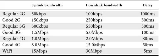
Table 3 lists the networking environments considered in this work. The settings and categorizations are based on the measure-ments given by an independent study [3]. Figure 4 shows the web-page rendering time with respect to the download time under each networking environment when using theinteractivegovernor. The download time dominates the end to end turnaround time for a 2G and a Regular 3G environments; and by contrast, the rendering time accounts for most of the turnaround time for a Good 4G and a WiFi environments when the delay is small.

In this work, we learn a predictor per optimization goal for each of the seven networking environments. Our framework allows new predictors to be added to target different environments and no retraining is required for existing predictors. Because the process of model training and data collection can be performed automatically, our approach can be easily ported to a new hardware platform or networking environment.

R e g u l a r 3 G R e g u l a r 4 G W i F i

0

4

8

1 2 1 6 2 0

O r a c l e

b e s t - p e r f o r m i n g e x i s t i n g ( C P U + G P U ) I n t e r . ( C P U ) + D e f a u l t ( G P U )

L

o

a

d

T

im

e

(s

)

(a) Load time

R e g u l a r 3 G R e g u l a r 4 G W i F i

0

5

1 0 1 5 2 0 2 5 3 0 3 5

O r a c l e

b e s t - p e r f o r m i n g e x i s t i n g ( C P U + G P U ) I n t e r . ( C P U ) + D e f a u l t ( G P U )

E

n

e

rg

y

(J

)

(b) Energy consumption

R e g u l a r 3 G R e g u l a r 4 G W i F i

0

3 0 6 0 9 0 1 2 0 1 5 0 1 8 0

O r a c l e

b e s t - p e r f o r m i n g e x i s t i n g ( C P U + G P U ) I n t e r . ( C P U ) + D e f a u l t ( G P U )

E

D

P

(J

*s

)

(c) EDP

Figure 2: The total load time (a), energy consumption (b) and energy delay product (EDP) (c) when a user was browsing four news pages fromnews.bbc.co.uk. We show the results fororacle, thebest-performingexisting CPU and GPU frequency governors,

andinteractive(CPU) +Default(GPU) in three typical networking environments. There is significant room for improvement.

Table 2: Optimal configurations forBBCpages. The color box highlights which CPU the rendering process should run on while each color code represents a specific CPU frequency.

Regular 3G Regular 4G WiFi

A15 (GHz) A7 (GHz) GPU (GHz) A15 (GHz) A7 (GHz) GPU (GHz) A15 (GHz) A7 (GHz) GPU (GHz)

Load time 1.7 0.4 0.543 1.8 0.4 0.600 1.8 0.4 0.600

Energy 0.4 0.8 0.400 0.4 0.8 0.400 0.8 0.4 0.543

Landing page

EDP 0.8 0.4 0.420 0.8 0.4 0.420 0.8 0.8 0.543

news page 1

Load time 1.6 0.4 0.543 1.6 0.4 0.600 1.7 0.4 0.600

Energy consumption 0.8 0.4 0.420 0.8 0.4 0.420 0.8 0.4 0.420

EDP 0.8 0.4 0.420 0.8 0.8 0.420 0.8 0.8 0.420

Load time 1.8 0.4 0.600 1.8 0.4 0.600 1.8 0.4 0.600

Energy consumption 0.8 0.4 0.420 0.8 0.8 0.420 1.2 0.4 0.543

sub-page 2

EDP 0.8 0.8 0.420 1.2 0.8 0.543 1.2 0.8 0.543

news page 3

Load time 1.6 0.4 0.543 1.7 0.4 0.600 1.8 0.4 0.600

Energy consumption 0.4 0.4 0.350 0.4 0.8 0.400 0.8 0.8 0.420

EDP 0.4 0.4 0.350 0.4 0.8 0.400 0.8 0.4 0.420

features values

Browser Extension

processor config.

Network Monitor

delay&bandwidth

scheduling

web contents

Predictive Model

<html> _... </html>

a b

Figure 3: Overview of our approach. The network moni-tor evaluates the network bandwidth and delay to choose a model to predict the oprimL processor configuration.

Table 3: Networking environment settings

Uplink bandwidth Downlink bandwidth Delay

Regular 2G 50kbps 100kbps 1000ms

Good 2G 150kbps 250kbps 300ms

Regular 3G 300kbps 550kbps 500ms

Good 3G 1.5Mbps 5.0Mbps 100ms

Regular 4G 1.0Mbps 2.0Mbps 80ms

Good 4G 8.0Mbps 15.0Mbps 50ms

WiFi 15Mbps 30Mbps 5ms

91._983.680.1

54.561.6

25.₂₂0.1

R . 2 G G . 2 G R . 3 G G . 3 G R . 4 G G . 4 G W i F i

0 %

2 0 %

4 0 %

6 0 %

8 0 %

1 0 0 %

R e n d e r i n g E n g i n e ( C P U ) a n d G P U P a i n t i n g D o w n l o a d

Figure 4: Webpage rendering and painting time w.r.t. content download time when using theinteractive(CPU) and the

Default(GPU) governors on Odriod Xu3.

distance,d, is calculated using the following formula:

d=α|db_m−db|+β|ub_m−ub|+γ|d_m−d| (1)

wheredbm,ubm, anddmare the measured downlink bandwidth,

Network-aware Web Browsing on Heterogeneous Mobile Systems CoNEXT ’18, Heraklion, Greece, 2018 <HTML> <HTML> <HTML> features values Browser Extension processor config. Network Monitor delay&bandwidth scheduling web contents Predictive Model <html> ... </html> a b Feature extraction

optimal proc. config.

webpage feature values Le ar n in g A lg o rit h m Predictor Training webpages Profiling runs <html> ... </html> <html> ... </html> <HTML> <HTML> Profiling runs Profiling runs

Optimal proc. config.

Learning Algorithm SVM <A15-0.2GHz, A7-0.2GHz> <A15-0.4GHz, A7-0.2GHz> <A15-2.0GHz, A7-1.4GHz>

Support Vector Machine

Predictor

Output

Profiling runs

Optimal proc. config. <A15-0.4GHz, A7-0.4GHz, GPU-0.355GHz>

<A15-0.8GHz, A7-0.4GHz, GPU-0.42GHz>

<A15-2.0GHz, A7-1.4GHz,GPU-0.6GHz>

Support Vector Machine

Extract features

Predictors

Output <HTML>

Training

webpages <HTML><HTML><HTML><HTML>

0.2GHz-1.2GHz ⁞ ⁞ 1.2GHz-2.0GHz

Least Energy: Optimal Load Time: Best EDP: 0.2GHz-1.2GHz ⁞ ⁞ 1.2GHz-2.0GHz ⁞ ⁞ <A15-0.4GHz, A7-0.4GHz> <A15-2.0GHz, A7-1.7GHz> <A15-0.8GHz, A7-0.4GHz> #DOM:1021 Depth of Tree: 11

#<li>:201 ⁞ ⁞ ⁞ ⁞ #DOM:1021 Depth of Tree: 11

#<li>:201

⁞

⁞

Least Energy: Optimal Load Time: Best EDP:

<A15-0.4GHz, A7-0.4GHz,GPU-0.355GHz> <A15-2.0GHz, A7-0.4GHz, GPU-0.6GHz>

<A15-0.8GHz, A7-0.4GHz,GPU-0.6GHz>

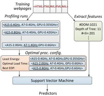
Figure 5: Learning predictive models using training data col-lected from a target network environment.

4.2

Training the Predictor

Figure 5 depicts the process of using training webpages to build a SVMclassifier for an optimization target under a networking envi-ronment. Training involves finding the best processor configuration and extracting feature values for each training webpage, and learn a model from the training data.

Generate Training Data.In this work, we used around 900 web-pages to train aSVMpredictor; we then evaluate the learnt model on the other 100 unseen webpages. These training webpages are selected from the landing page of the top 1000 hottest websites ranked bywww.alexa.com(see Section 5.2). We use Netem [24], a Linux-based network enumerator, to emulate various networking environments to generate the training data (see also Section 5.1). We exhaustively execute the rendering engine and painting process under different processor settings and record the optimal configura-tion for each optimizaconfigura-tion goal and each networking environment. We then assign each optimal configuration a unique label. For each webpage, we also extract values of a set of selected features and store the values in a fixed vector (see Section 4.3).

Building The Model.The feature values together with the labeled processor configuration are supplied to a supervised learning al-gorithm [29]. The learning alal-gorithm tries to find a correlation from the feature values to the optimal configuration and produces aSVMmodel per networking environment per optimization goal. Because we target three optimization metrics and seven network-ing environments, we have constructed 21SVMmodels in total for a given platform. An alternative is to have a single model for all optimization metrics and networking environments. However, this strategy requires retraining the model when targeting a new metric or environment and thus incurs extra training overheads. Training Cost.The training time of our approach is dominated by generating the training data. In this work, it takes less than a week to collect all the training data. In comparison processing the

HTML web contents

Parsing

DOM tree & style rules

feature values Predictor processor config. Scheduling CSS 1 3 Network Profiling delay &bandwidth 2 features values Predictvie model processor config. Network Monitor delay&bandwidth web contents delay&bandwidth DOM tree scheduling web server web contents Parsing PC1 (47%) PC2 (11.4%) PC3 (7.2%) PC4 (5.8%) PC5 (4.4%) PCs 6-8

(9.1%) PCs 9-18

(9.7%) Rest PCs -5%

(a) Principal components

w eb p a ge s

i z e

# DO M n od e

d ep t h o f t r e

e

# At t r . s t yl e

# Ta g . l i nk

# Ta g . s cr i p

t

# Ta g . i mg 0 %

1 0 % 2 0 % 3 0 %

% o f c on tri . t o va ria nc e

(b) Top 7 most important features

Figure 6: The percentage of principal components (PCs) to the overall feature variance (a), and contributions of the seven most important raw features in thePCAspace (b).

raw data, and building the models took a negligible amount of time, less than an hour for learning all individual models on a PC. Since training is only performed once at the factory, it is aone-offcost.

4.3

Web Features

One of the key aspects in building a successful predictor is finding the right features to characterize the input workload. In this work, we consider a set of features extracted from the web contents. These features are collected by our feature extraction pass. To gather the feature values, the feature extractor first obtains a reference for each DOMelement by traversing theDOMtree and then uses the Chromium API,document.getElementsByID, to collect node information.

We started from 214 raw features, including the number ofDOM nodes, HTML tags and attributes of different types, and the depth of theDOMtree, etc. All these features can be collected at the parsing time from the browser. The types of the raw features are given in Table 4. Some of these features are selected based on our intuition what may be important for our problem, while others are chosen based on prior work [9, 36, 40]. It is important to note that the collected feature values are encoded to a vector of real values. One of the advantages of our web features is that the feature values are obtained at the very beginning of the loading process, which gives enough time for runtime optimization.

Table 4: Raw web feature categories

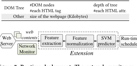
DOM Tree #DOM nodes depth of tree #each HTML tag #each HTML attr. Other size of the webpage (Kilobytes)

Run-time scheduler

Extension

Feature normalization

SVM predictor Network

Monitor

web

contents Feature

extraction Web

Server

Figure 7: Runtime deployment. The network monitor re-ports the network status. A model is chosen based on the network and optimization goal to predict the processor con-figuration, which is then passed to the runtime scheduler.

Feature Normalization.Before passing our features to a machine learning model we need to scale each of the features to a common range (between 0 and 1) in order to prevent the range of any single feature being a factor in its importance. Scaling features does not affect the distribution or variance of their values. To scale the fea-tures of a new webpage during deployment we record the minimum and maximum values of each feature in the training dataset, and use these to scale the corresponding features.

Feature Analysis.To understand the usefulness of each raw fea-ture, we apply the Varimax rotation [33] to thePCAspace. This technique quantifies the contribution of each feature to eachPC. Figure 6b shows the top 7 dominant features based on their contri-butions to thePCs. Features like the webpage size and the number ofDOMnodes are most important, because they strongly correlate with the download time and the complexity of the webpage. Other features like the depth of theDOMtree, and the numbers of different attributes and tags, are also useful, because they determine how the webpage should be presented and how do they correlate to the rendering cost. The advantage of our feature selection process is that it automatically determines what features are useful when targeting a new hardware platform where the relative cost of page rendering and the importance of features may change.

4.4

Runtime Deployment

Once we have built the predictive models described above, we can use them for anynew,unseenwebpage. Figure 7 illustrates the steps of runtime prediction and task scheduling. The network monitor reports the network bandwidths and delay, which are used to deter-mine the runtime status. The web browser then selects a predictor to use based on the network status and the optimization goal. Dur-ing the parsDur-ing stage, which takes less than 1% of the total renderDur-ing time [34], the feature extractor firstly extracts and normalizes the feature values. Next, the selected predictive model predicts the opti-mal processor frequency based on the feature values. The prediction is then passed to the runtime scheduler to perform task scheduling and hardware configuration. The overhead of network monitoring, extracting features, prediction and configuring frequency is small. It is less than 7% of the turnaround time (see also Section 6.3.3),

which is included in all our experimental results.

Table 5: None-zero feature values forGooglesearch (p1), the

result page (p2) and the target website (p3).

Feature Raw value Normalized value

p1 p2 p3 p1 p2 p3

#DOMnodes 397 1292 4798 0.049 0.163 0.611 depth of tree 21 13 23 0.750 0.416 0.833 #img 3 5 169 0.004 0.007 0.256 #li 19 76 799 0.011 0.046 0.490 #link 2 8 3 0.026 0.106 0.04 #script 13 79 54 0.099 0.603 0.412 #href 46 155 2044 0.022 0.075 0.99 #src 3 21 84 0.006 0.043 0.167 #content 2 23 11 0.039 0.450 0.215

As theDOMtree is constructed incrementally by the parser, it can change throughout the duration of rendering. To make sure that our approach can adapt to the change of available information, re-prediction and rescheduling will be triggered if theDOMtree is significantly different from the one used for the last prediction. The difference is calculated by counting the number ofDOMnodes between the previous and the currentDOMtrees. If the difference is greater than 30%, we will make a new prediction using feature values extracted from the currentDOMtree. We have observed that our initial prediction often remains unchanged, so rescheduling and reconfiguration rarely happened in our experiments.

4.5

Example

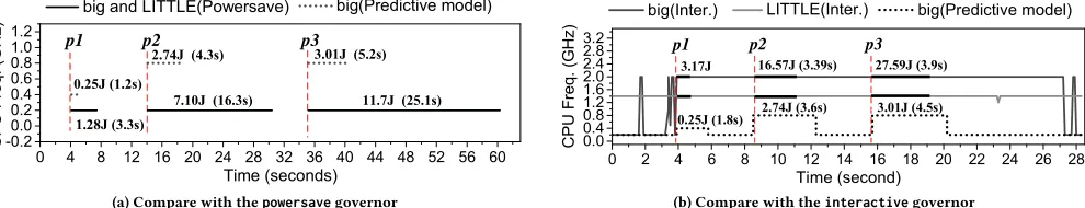
To demonstrate how our approach works, we now consider a sce-nario where a user conducts a search onGoogleto look for an online service. There are three webpages to be rendered in this process: theGooglesearch page, the search result page, and the target website, which are denoted asp1,p2andp3respectively. Here we assume the user uses a Regular 3G network and wants to retrieve the information with minimum energy usage by informing the system via e.g., choosing the battery saver mode on Android.

Network-aware Web Browsing on Heterogeneous Mobile Systems CoNEXT ’18, Heraklion, Greece, 2018

0 2 4 6 8 10 12 14 16 18 20 22 24 26 28

0.0 0.8 1.6 2.4 3.2

LITTLE(Inter.) big(Predictive model)

C P U F re q . ( G H z) Time (second) big(Inter.)

0 2 4 6 8 10 12 14 16 18 20 22 24 26 28

0.0 0.3 0.6 0.9 1.2 1.5 1.8 2.1 2.4 2.7 3.0 3.3 CPU F req ue ncy(G H z) Time(second) big(Interactive) LITTLE(Interactive) big(predictive model) 0.25J 3.17J 16.57J 2.74J 27.59J 3.01J

p1 p2 p3

0 2 4 6 8 10 12 14 16 18 20 22 24 26 28

0.0 0.4 0.8 1.2 1.6 2.0 2.4 2.8

3.2 LITTLE(Inter.) big(Predictive model)

C P U F req uency( G H z) Time(second) big(Inter.) 0.25J (1.8s) 3.17J (0.78s) 16.57J (3.39s) 2.74J (3.6s) 27.59J (3.9s) 3.01J (4.5s) p2 p3 p1

0 4 8 12 16 20 24 28 32 36 40 44 48 52 56 60

0.0 0.3 0.6 0.9 1.2

1.5 big(predictive model)

C P U Fr equency (G Hz) Time(second)

big and LITTLE(Powersave)

0.25J

7.10J 2.74J

11.7J 3.01J

0 4 8 12 16 20 24 28 32 36 40 44 48 52 56 60

0.0 0.3 0.6 0.9 1.2 1.5 CPU F req ue ncy(G H z) Time(second)

big and LITTLE(Powersave) big(predictive model) p1 p2 p3 0.25J _7.10J 2.74J 11.7J 3.01J p2 p3 1.28J

0 4 8 12 16 20 24 28 32 36 40 44 48 52 56 60

0.0 0.3 0.6 0.9 1.2

1.5 big(predictive model)

C P U Fr eque ncy( G H z) Time(second) big and LITTLE(Powersave)

p1 0.25J (1.2s) 7.10J (16.3s) 2.74J (4.3s) 11.7J (25.1s) 3.01J (5.2s) p2 p3 1.28J(3.3s)

0 4 8 12 16 20 24 28 32 36 40 44 48 52 56 60

0.0 0.3 0.6 0.9 1.2 1.5 CP U Fr eq . ( GHz) big(Predictive model) Time(second) big and LITTLE(Powersave) p1

0.25J (1.2s)

7.10J (16.3s) 2.74J (4.3s)

11.7J (25.1s) 3.01J (5.2s)

p2 p3

1.28J (3.3s)

0 2 4 6 8 10 12 14 16 18 20 22 24 26 28

0.0 0.8 1.6 2.4 3.2

LITTLE(Inter.) big(Predictive model)

CP U F req. (G Hz ) Time(second) big(Inter.) 0.25J (1.8s) 3.17J (0.78s) 16.57J (3.39s) 2.74J (3.6s) 27.59J (3.9s) 3.01J (4.5s)

p1 p2 p3

0 4 8 12 16 20 24 28 32 36 40 44 48 52 56 60

0.0 0.3 0.6 0.9 1.2 1.5 CP U Fr e q. (G Hz

) big(Predictive model)

Time (second) big and LITTLE(Powersave)

0 4 8 12 16 20 24 28 32 36 40 44 48 52 56 60

0.0 0.3 0.6 0.9 1.2 1.5 CPU Freq . (G H z) big(Predictive model) Time (second) big and LITTLE(Powersave)

0.25J (1.2s)

7.10J (16.3s) 2.74J (4.3s)

11.7J (25.1s) 3.01J (5.2s)

p2 p3

1.28J (3.3s)

p1

0 4 8 12 16 20 24 28 32 36 40 44 48 52 56 60

-0.20.0 0.2 0.4 0.6 0.8 1.0 1.2 C P U F req. (GH z) big(Predictive model) Time (seconds) big and LITTLE(Powersave)

(a) Compare with thepowersavegovernor

0 2 4 6 8 10 12 14 16 18 20 22 24 26 28 0.0 0.4 0.8 1.2 1.6 2.0 2.4 2.8 3.2

LITTLE(Inter.) big(Predictive model)

CPU F

req. (G

Hz)

Time (second) big(Inter.)

0 2 4 6 8 10 12 14 16 18 20 22 24 26 28 0.0 0.4 0.8 1.2 1.6 2.0 2.4 2.8 3.2

LITTLE(Inter.) big(Predictive model)

CPU F re q . ( G H z) Time (second) big(Inter.)

0 2 4 6 8 10 12 14 16 18 20 22 24 26 28 0.0

0.8 1.6 2.4 3.2

LITTLE(Inter.) big(Predictive model)

CP U F req . ( G Hz ) Time (second) big(Inter.)

0 2 4 6 8 10 12 14 16 18 20 22 24 26 28

0.0 0.3 0.6 0.9 1.2 1.5 1.8 2.1 2.4 2.7 3.0 3.3 CPU Frequ enc y( GH z) Time(second) big(Interactive) LITTLE(Interactive) big(predictive model) 0.25J 3.17J 16.57J 2.74J 27.59J 3.01J

p1 p2 p3

0 2 4 6 8 10 12 14 16 18 20 22 24 26 28 0.0 0.4 0.8 1.2 1.6 2.0 2.4 2.8

3.2 LITTLE(Inter.) big(Predictive model)

C P U Fr eq uenc y( G H z) Time(second) big(Inter.) 0.25J (1.8s) 3.17J (0.78s) 16.57J (3.39s) 2.74J (3.6s) 27.59J (3.9s) 3.01J (4.5s) p2 p3 p1

0 4 8 12 16 20 24 28 32 36 40 44 48 52 56 60 0.0

0.3 0.6 0.9 1.2

1.5 big(predictive model)

CP U Fr equ enc y( GH z) Time(second)

big and LITTLE(Powersave)

0.25J

7.10J 2.74J

11.7J 3.01J

0 4 8 12 16 20 24 28 32 36 40 44 48 52 56 60

0.0 0.3 0.6 0.9 1.2 1.5 C P U Fr e que nc y( GH z) Time(second)

big and LITTLE(Powersave) big(predictive model) p1 p2 p3 0.25J 7.10J 2.74J 11.7J 3.01J p2 p3 1.28J

0 4 8 12 16 20 24 28 32 36 40 44 48 52 56 60 0.0

0.3 0.6 0.9 1.2

1.5 big(predictive model)

C P U Fr equen cy( G H z) Time(second) big and LITTLE(Powersave)

p1 0.25J (1.2s) 7.10J (16.3s) 2.74J (4.3s) 11.7J (25.1s) 3.01J (5.2s) p2 p3 1.28J(3.3s)

0 4 8 12 16 20 24 28 32 36 40 44 48 52 56 60 0.0 0.3 0.6 0.9 1.2 1.5 CP U Fr eq . (G Hz) big(Predictive model) Time(second) big and LITTLE(Powersave)

p1

0.25J (1.2s)

7.10J (16.3s) 2.74J (4.3s)

11.7J (25.1s) 3.01J (5.2s)

p2 p3

1.28J (3.3s)

0 2 4 6 8 10 12 14 16 18 20 22 24 26 28 0.0

0.8 1.6 2.4 3.2

LITTLE(Inter.) big(Predictive model)

CP U F req. ( G H z) Time(second) big(Inter.) 0.25J (1.8s)

3.17J 16.57J (3.39s)

2.74J (3.6s)

27.59J (3.9s)

3.01J (4.5s)

p1 p2 p3

0 4 8 12 16 20 24 28 32 36 40 44 48 52 56 60 0.0 0.3 0.6 0.9 1.2 1.5 C PU F req. ( GH z) big(Predictive model) Time (second) big and LITTLE(Powersave)

0 4 8 12 16 20 24 28 32 36 40 44 48 52 56 60 0.0 0.3 0.6 0.9 1.2 1.5 CP U Fr eq . (G Hz) big(Predictive model) Time (second) big and LITTLE(Powersave)

0.25J (1.2s)

7.10J (16.3s) 2.74J (4.3s)

11.7J (25.1s) 3.01J (5.2s)

p2 p3

1.28J (3.3s)

p1

0 4 8 12 16 20 24 28 32 36 40 44 48 52 56 60 -0.20.0 0.2 0.4 0.6 0.8 1.0 1.2 CP U Fre q. ( G Hz) big(Predictive model) Time (seconds) big and LITTLE(Powersave)

(0.78s)

0.25J (1.8s)

3.17J 16.57J (3.39s)

2.74J (3.6s)

27.59J (3.9s)

3.01J (4.5s)

p1 p2 p3

(b) Compare with theinteractivegovernor

Figure 8: The selected processor and CPU frequencies when renderingGooglesearch (p1), the search result page (p2), and the

target website (p3). We compare our approach againstpowersave(a) andinteractive(b) in a regular 3G environment.

Table 6: Hardware platforms

Odroid Xu3 Jetson TX2

big CPU 32bit quad-core Cortex-A15 @ 2GHz 64bit quad-core Cortex-A57 @ 2.0 GHz LITTLE CPU 32bit quad-core Cortex-A7 @ 1.4GHz 64bit dual-core Denver2 @ 2 GHz

GPU 8-core Mali-T628 @ 600MHz 256-core NVIDIA Pascal @ 1.3GHz

Figure 8a compares thepowersaveCPU frequency governor with our approach. This strategy runs all cores at the lowest fre-quency, 200MHz, aiming to minimize the system’s power consump-tion. However, running the processors at this frequency prolongs the page load time, which leads to over 1.59x (up to 4.12x) more energy consumption than our approach.

In contrast to the fixed strategy used bypowersave, the widely usedinteractivegovernor dynamically adjusts the processor fre-quency according to the user activities. From Figure 8b, we see that interactiveraises the big core frequency as soon as the browser starts fetchingp1. After that all cores stay on the highest frequency until a few seconds after the third webpage has been completely rendered. Whileinteractivecan choose CPU frequencies from the entire spectrum, it mostly focuses on the highest and the low-est frequencies. By contrast, our approach dynamically adjusts the processor frequency according to the web content and browsing activities. It chooses to operate the processors at 400MHz for the relatively simplep1 page that has the smallest number ofDOMnodes, and then raises the frequency up to 800MHz for the next two more complex pages. As a result, our approach reduces the energy con-sumption by 87% at the cost of 22% slower when compared with interactive. Considering the goal is to minimize the energy con-sumption, our approach outperformsinteractiveon this task.

5

EXPERIMENTAL SETUP

5.1

Hardware and Software Platform

Evaluation Platform.To demonstrate the portability, we evalu-ate our approach on two distinct mobile platforms, Odriod XU3 Jetson TX2. Table 6 gives detailed information of both platforms. We chose these platforms as they are a representative big.LITTLE embedded architecture and has on-board energy sensors for power measurement. Both systems run Ubuntu 16.04 with the big.LITTLE enabled scheduler. We used the on board energy sensors and ex-ternal power monitor to measure the energy of theentiresystem.

These sensors have been checked against external power measure-ment instrumeasure-ments and proven to be accurate in prior work [27]. We implemented our approach in Google Chromium (version 64.0) which is compiled using the gcc compiler (version 7.2).

Networking Environments.To ensure that our results are re-producible, we use a Linux server to record and replay the server responses through the Web Page Replay tool [2]. Our mobile test board and the web server communicate through WiFi, but we use Netem [24] to control the network delay and server bandwidth to simulate the seven networking environments defined in Table 3. We add 30% of variances (which follow a normal distribution) to the bandwidths, delay and packet loss to simulate a dynamic network environment. Note that we ensure that the network variances are the same during the replay of a test page. We also measure the difference of power between the WiFi and the cellular interfaces, and use this to calibrate the energy consumption in cellular environ-ments. Finally, unless stated otherwise, we disabled the browser’s cache to provide a fair comparison across different methods (see also Section 6.2).

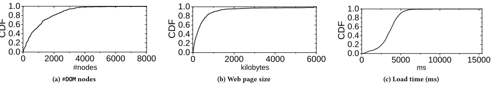
Workloads.We used the landing page of the top 1,000 hottest websites fromwww.alexa.com. We include both the mobile and the desktop versions of the websites, because many mobile users still prefer the desktop-version for their richer content and experi-ence [13]. Figure 9 shows the CDF of the number ofDOMnodes, web content sizes and load time when using theinteractivegovernor in a WiFi environment. TheDOMnode and webpage sizes range from small (4DOMnodes and 40 KB) to large (over 8,000DOMnodes and 6 MB), and the load time is between 0.13 second and 15.4 seconds, suggesting that our test data cover a diverse set of web contents.

5.2

Evaluation Methodology

0 2 0 0 0 4 0 0 0 6 0 0 0 8 0 0 0 0 . 0

0 . 2 0 . 4 0 . 6 0 . 8 1 . 0

C

D

F

# n o d e s

(a) #DOMnodes

0 2 0 0 0 4 0 0 0 6 0 0 0 0 . 0

0 . 2 0 . 4 0 . 6 0 . 8 1 . 0

k i l o b y t e s

C

D

F

(b) Web page size

0 5 0 0 0 1 0 0 0 0 1 5 0 0 0 0 . 0

0 . 2 0 . 4 0 . 6 0 . 8 1 . 0

C

D

F

m s

(c) Load time (ms)

Figure 9: The CDF of #DOMnodes (a), webpage size (b), and load time when usinginteractivein a WiFi network (c).

Existing Frequency Governors.We compare our approach against existing CPU and GPU frequency governors. Specifically, we con-sider five widely used CPU governors:interactive,powersave, performance,conservative, andondemand. For GPUs, we con-sider three purpose-built governors for the ARM Mali GPU (Odroid Xu3):Default,StaticandBooster, and three others for the NVIDIA Pascal GPU (Jetson TX2):nvhost_podgov,simple_ondemandand userspace. We useinteractiveas the baseline CPU governor, andDefaultandnvhost_podgovas the baseline GPU governor on Odroid Xu3 and Jetson TX2, respectively.

Competitive Approaches.We compare our approach with two state-of-the arts: a web-aware scheduling mechanism (termed as WS) [55] and a machine learning based web browser scheduling scheme (termed asS-ML) [40].WSuses a regression model to esti-mate webpage load time and energy consumption under different processor configurations. The model is then used as a cost function to find the best configuration by enumerating all possible configu-rations.S-MLalso develops a machine learning classifier to predict the optimal processor configuration, but it assumes that all the webpages have been pre-downloaded and ignores the impact of the dynamic network environments. We trainWSandS-MLusing the same training dataset as the one we used to train our models in a WiFi environment (which is the networking environment used by both methods for collecting training data)

Performance Report.We report thegeometric meanof each eval-uation metric across evaleval-uation scenarios. The geometric mean is a widely used performance metric. Compared to the arithmetic mean, it can better minimize the impact of performance outliers – which could make the results look better than they are [19]. To collect run-time and energy consumption, we run each model on each input repeatedly until the 95% confidence bound per model per input is smaller than 5%. For load time, we instrumented Chromium to measure the wall clock time between theNavigation Start and theLoad Event Endevents. We excluded the time spent on browser bootstrap and shut down. To measure the energy consump-tion, we developed a lightweight runtime to take readings from the on-board energy sensors at a frequency of 100 samples per second. We then matched the energy readings against the time stamps of webpage rendering to calculate the energy consumption.

6

EXPERIMENTAL RESULTS

Highlights of our evaluation are as follows:

• Our approach consistently outperforms the existing Linux-based governors across networking environments, optimiza-tion goals, and hardware platforms. See Secoptimiza-tion 6.1;

• Our approach gives better and more stable performance com-pared to state-of-the-art web-aware schedulers (Section 6.2);

• We thoroughly evaluate our approach and provide detailed analysis on its working mechanisms (Section 6.3).

6.1

Overall Results

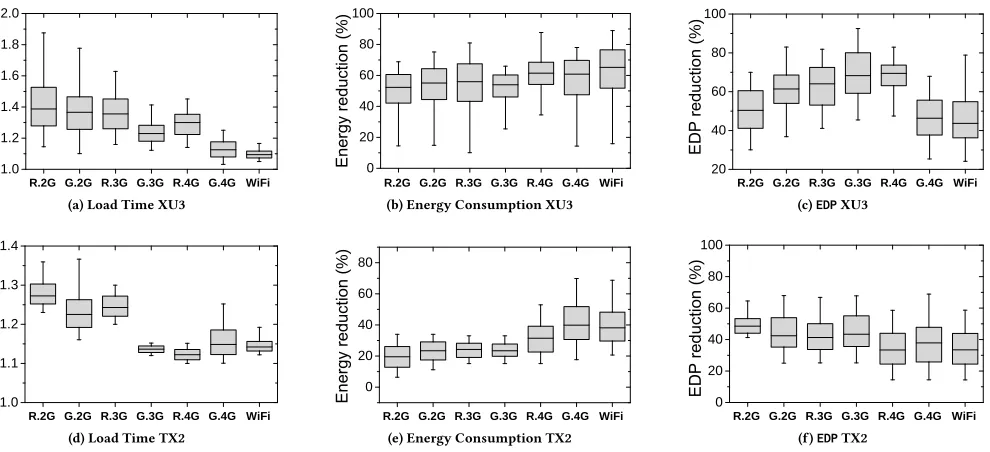
The box-plot in Figure 10 depicts the improvements of our approach over the best-performing Linux-based CPU and GPU governor. The min-max bars show the range of improvements achieved across webpages.

Network-aware Web Browsing on Heterogeneous Mobile Systems CoNEXT ’18, Heraklion, Greece, 2018

R . 2 G G . 2 G R . 3 G G . 3 G R . 4 G G . 4 G W i F i 1 . 0

1 . 2 1 . 4 1 . 6 1 . 8 2 . 0

Lo

ad

ti

m

e

im

pr

ov

em

en

t

(

x

)

(a) Load Time XU3

R . 2 G G . 2 G R . 3 G G . 3 G R . 4 G G . 4 G W i F i

0

2 0 4 0 6 0 8 0 1 0 0

E

ne

rg

y

re

du

ct

io

n

(

%

)

(b) Energy Consumption XU3

R . 2 G G . 2 G R . 3 G G . 3 G R . 4 G G . 4 G W i F i 2 0

4 0 6 0 8 0 1 0 0

E

D

P

re

du

ct

io

n

(

%

)

(c)EDPXU3

R . 2 G G . 2 G R . 3 G G . 3 G R . 4 G G . 4 G W i F i 1 . 0

1 . 1 1 . 2 1 . 3 1 . 4

Lo

ad

ti

m

e

im

pr

ov

em

en

t

(

x

)

(d) Load Time TX2

R . 2 G G . 2 G R . 3 G G . 3 G R . 4 G G . 4 G W i F i

0

2 0 4 0 6 0 8 0

E

ne

rg

y

re

du

ct

io

n

(

%

)

(e) Energy Consumption TX2

R . 2 G G . 2 G R . 3 G G . 3 G R . 4 G G . 4 G W i F i

0

2 0 4 0 6 0 8 0 1 0 0

E

D

P

re

du

ct

io

n

(

%

)

(f)EDPTX2

Figure 10: Improvement achieved by our approach over the best-performing Linux CPU governor for load time, energy re-duction andEDPon Odroid XU3 and Jetson TX2. The min-max bars show the range of performance improvement across web-pages. Our approach consistently outperforms the best-performing Linux-based governors across networking environments, optimization goals and hardware platforms.

Linux governor by using less than 31% to 55% (up to 88%) energy consumption across networking environments. It is worth men-tioning that our approach never consumes more energy compared to other Linux governors, because it correctly selects the optimal (or near optimal) frequency and the best core to run the rendering process.

EDP.Figure 10c shows the results forEDP, a metric for quantifying the trade-off between energy and response time. A lowEDPvalue means that energy consumption is reduced at the cost of little impact on the response time. Our approach successfully cuts down theEDPacross networking environments. We observe significant improvement is available in a 3G and a Regular 4G environments, where our approach gives over 60% and 30% reduction onEDP for Odroid XU3 and Jetson TX2, respectively. Our approach also reduces theEDPby over 30% in other networking environments. Once again, our approach outperforms the best-performing Linux governor for all the test cases onEDP.

6.2

Compare to Competitive Approaches

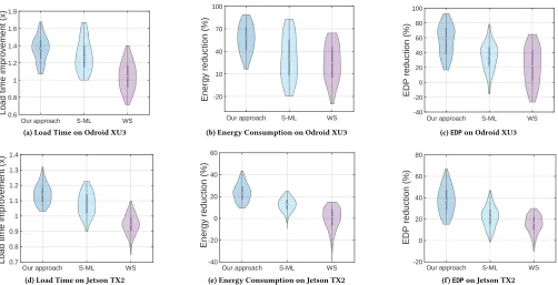
The violin plot in Figure 11 compares our approach against two state-of-the-arts,S-MLandWS, across networking environments and webpages on Odroid XU3 and Jetson TX2, respectively. The baseline is the best-performing Linux CPU and GPU governor found for each webpage. The width of each violin corresponds to the proportions of webpages with a certain improvement. The white dot denotes the median value, while the thick black line shows where 50% of the data lies.

Our approach S-ML WS 0.6

0.8 1 1.2 1.4 1.6 1.8

Load time improvement (x)

(a) Load Time on Odroid XU3

Our approach S-ML WS

-20 10 40 70 100

Energy reduction (%)

(b) Energy Consumption on Odroid XU3

Our approach S-ML WS

-40 -20 0 20 40 60 80 100

EDP reduction (%)

(c)EDPon Odroid XU3

Our approach S-ML WS

0.7 0.8 0.9 1 1.1 1.2 1.3 1.4

Load time improvement (x)

(d) Load Time on Jetson TX2

Our approach S-ML WS

-40 -20 0 20 40 60

Energy reduction (%)

(e) Energy Consumption on Jetson TX2

Our approach S-ML WS

-20 0 20 40 60 80

EDP reduction (%)

(f)EDPon Jetson TX2

Figure 11: Violin plots showing the distribution for our approach,S-MLandWSin different network environments for three evaluation metrics on Odroid XU3 and Jetson TX2. The baseline is the best-performing Linux-based CPU and GPU governor. The thick line shows where 50% of the data lies. The white dot is the position of the median. Our approach delivers the best and most stable performance across testing scenarios.

approach has a better performance on Odroid XU3 than Jetson TX2 across all metrics, because of the performance of the big.LITTLE cores on Jetson TX2, A57 (big) and Denver 2 (little), has less differ-ences than the processors’ on Odroid XU3, for example, the Denver 2 and A57 have the similar frequency domain (as Table 6 shows), and the predicted model can not take full advantage of the low power property on little cores.

In contrast to other two adaptice approaches, our machine learn-ing approach is more stable. On average, we achieve by 17%, 31% and 30% improvement respectively for load time, energy consumption and EDP across all networks, metrics and platforms.

6.3

Model Analysis

6.3.1 Optimal configurations.Figure 12 shows the

distribu-tion of optimal processor configuradistribu-tions found through exhaustive search on Odroid XU3 and Jetson TX2. Here, we use the notation <CPU render core - bigfreq, littlefreq, GPU-freq>to denote a processor configuration, where the core that the rendering process runs on is placed at the beginning, and the painting frequency is located at the last. For example,<A15 - 1.6, 0.4, GPU-1.1>means that the rendering process running on the A15 core (big core) at 1.6GHz and the A7 core (little core) runs at 400MHz, and the paint-ing process runnpaint-ing on the GPU at 1.1GHz.

As can be seen from Figure 12a and Figure 12d, when optimizing for load time, the rendering engine should run on the big core (A15, A57) to provide high performance to Odroid XU3 and Jetson TX2.

However, the optimal frequency varies across networking environ-ments and we see the change of distribution in frequencies when moving from a slow network to a fast one. For instance, on Odroid XU3, while it is unprofitable to run the A15 core at 1.9GHz and GPU at 0.6GHz in a slow network, it is the desired frequency for 68% of the webpages in a WiFi environment. When optimizing for energy consumption (Figure 12b and Figure 12e) andEDP(Figure 12c and Figure 12f), it can be beneficial to run the rendering process on the energy-tuned core (A7, D2). For example, in a 2G environment, running the rendering process on the A7 core with a frequency of 400MHz or 800MHz benefits up to 46% of webpages, although the distribution changes across networks and optimization metrics. If we compare the distributions across networks and metrics, we find that the best core for running the rendering process and the frequency varies across networking environments, webpages and optimization goals. The results reinforce our claim that the sched-uling policy must be aware of the networking environment, web contents and the optimization target.

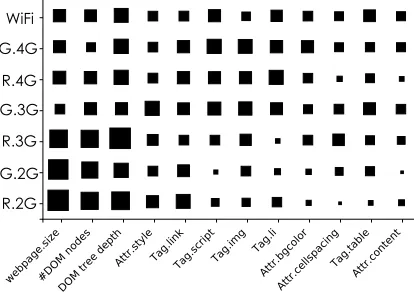
6.3.2 Feature Importance. Section 4.3 has shown the

Network-aware Web Browsing on Heterogeneous Mobile Systems CoNEXT ’18, Heraklion, Greece, 2018

$

*38!$*38!$*38! $*38!

5* ** 5* ** 5* **

:L)L

(a) Load Time on Odroid Xu3

$

*38!$*38!$*38!$*38!$*38!

5* ** 5* ** 5* **

:L)L

(b) Energy Consumption on Odroid Xu3

$

*38!$*38!$*38!$*38!$*38!

5* ** 5* ** 5* **

:L)L

3HUFHQWDJH

(c)EDPon Odroid Xu3

$_*38!$_*38!$_*38!$_*38!$_*38!

5* ** 5* ** 5* **

:L)L

(d) Load Time on Jetson TX2

'

*38!'*38!$*38!$*38!$*38! 5*

** 5* ** 5* **

:L)L

(e) Energy Consumption on Jetson TX2

'

*38!'*38!$*38!$*38!$*38!

5* ** 5* ** 5* **

:L)L

3HUFHQWDJH

(f)EDPon Jetson TX2

Figure 12: The distributions of optimal process configurations for load time, energy consumption andEDPon Odroid XU3 and Jetson TX2. The distribution of optimal configuration changes across environments, showing the need of an adaptive scheme.

models for the seven networking environments. The importance is calculated through the information gain ratio. It can be observed that HTML tags and attributes (e.g. webpage size, #DOM nodes , DOM tree depth) and style rules are important when determining the processor configurations for all networking environments. We can also see such features play an more important role for 2G and regular 3G than others. Other features are extremely important for some networks (such as the number HTML tags of<Tag.script> and<Tag.li>are important for WiFi, 4G and good 3G,) but less important for others. This diagram illustrates the need for a distinct model for each optimization goal and how important it is to have an automatic technique to construct such models.

6.3.3 Breakdown of Overhead.Figure 14 shows the overhead

of our approach (which is already included in our experimental results). Our approach introduces little overhead to the end to end turnaround time and energy consumption, less than 7% and 5% respectively. The majority of the time and energy are spent on network monitoring for measuring the network delay and band-widths. The overhead incurred by the browser extension and the runtime scheduler, which includes task migration, feature extrac-tion, making prediction and setting processor frequencies, is less than 0.8%, with task migration (around 10ms) accounts for most of the overhead. As can be seen from the better aforementioned results, the overhead of our approach can be amortized by the improved performance.

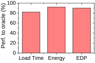
6.3.4 Oracle performance. Figure 15 compares our approach

with theoraclepredictor, showing how close our approach is to the theoretically perfect solution. Our approach achieves 82%,

webpage.size#DOM nodes_{DOM tree depth}Attr.styleTag.linkTag.scriptTag.img Tag.li

Attr.bgcolor Attr.cellspacing

Tag.table_Attr.content WiFi

G.4G R.4G G.3G R.3G G.2G R.2G

Figure 13: A Hinton diagram shows the importance of the selected web feature to the prediction accuracy under differ-ent networks. The larger the box, the more likely a feature affects the prediction accuracy of the respective model.

92% and 90% of theoracle performance for load time, energy consumption, andEDPrespectively. Overall, the performance of our approach is not far from theoracle.

6.3.5 Prediction accuracy.Our approach gives correct

L o a d T i m e E n e r g y C o n s u m p t i o n

0

1

2

3

4

5

6

7

8

9

1 0

N e t w o r k M o n i t o r E x t e n s i o n + S c h e d u l e r

O

v

e

rh

e

a

d

(

%

)

Figure 14: Breakdown of runtime overhead. Our approach incurs little runtime overhead.

L o a d T i m e E n e r g y

E D P

0

2 0 4 0 6 0 8 0 1 0 0

P

e

rf

.

to

o

ra

c

le

(

%

)

Figure 15: Performance of our approach w.r.t.oracle. Our approach delivers over 80% of theoracleperformance

L o a d T i m e E n e r g y E D P

0

2 0 4 0 6 0 8 0 1 0 0

K N N M L P S V M N B L R A N N

P

e

rf

.

to

o

ra

c

le

(

%

)

Figure 16: The performance w.r.toracleachieved by ourSVM

based approach and other classification techniques.

6.3.6 Alternative modeling techniques.Figure 16 shows the

per-formance achieved by our approach and five widely used classi-fication techniques with respect to theoracleperformance. The alternative classifiers are: Multi-layer Perceptron (MLP), K-Nearest Neighbours (KNN), Artificial Neural Networks (ANN), Logistic Regres-sion (LR), and Naïve Bayes (NB). Each of the alternative modeling techniques were trained and evaluated by using the same method and training data as our model. Our approach outperforms all other alternative techniques for every optimization metric. It is worth noting that the performance of these competitive modeling tech-niques may improve if there are more training examples to support the use of a larger set of features. However, we found thatSVMs perform well on the training data we have.

7

RELATED WORK

Our work builds upon the following techniques, while qualitatively differing from each.

Web Browsing Optimization.Numerous techniques have been proposed to optimize web browsing, through e.g. prefetching [49] and caching [37] web contents, scheduling network requests [38], or re-constructing the browser workflow [32, 53] or the TCP pro-tocol [51]. Most of the prior work target homogeneous systems and do not optimize across networking environments. The work presented by Zhuet al.[55] and prior work [40] were among the first attempts to optimize web browsing on heterogeneous mobile systems. Both approaches use statistical learning to estimate the optimal configuration for a given web page. However, they do not consider the impact of the networking environment, thus miss mas-sive optimization opportunities. Buiet al.[14] proposed several web page rendering techniques to reduce energy consumption for mobile web browsing. Their approach uses analytical models to determine which processor core (big or little) to use to run the rendering process. The drawback of using an analytical model is that the model needs to be manually re-tuned for each individual platform to achieve the best performance. Our approach avoids the pitfall by developing an approach to automatically learn how to best schedule rendering process. As this work focuses on rendering process mapping, other optimization techniques proposed in [14], such as dynamic buffering, are complementary to our work. Task Scheduling. There is an extensive body of work on task scheduling on homogeneous and heterogeneous multi-core systems [10, 20, 35, 44, 52]. Most of the prior work in the area use heuristics or analytical models to determine which processor to use to run an application task, by exploiting the code or runtime information of the program. Our approach targets a different domain by using the web workload characteristics to optimize mobile web browsing across networking environments and optimization objectives. Energy Optimization.Techniques have been proposed to opti-mize web browsing via application-level optimization, including aggregating data traffic [12, 26, 47] or requests [11, 31], and parallel downloading [8, 25]. Our approach targets a lower level, by exploit-ing the heterogeneous hardware architecture to perform energy optimization. There is also an intensive body of research on web workload characterization [9, 15, 17]. The insights found from these studies can help us to better extract useful web features.

Predictive Modeling.Recent studies have shown that machine learning based techniques are effective in predicting power con-sumption [42], estimating mobile traffic [41], parallelism mapping [45], and processor resource allocation [50]. No work so far in the area has used machine learning to predict the optimal processor config-uration for mobile web browsing by exploiting the knowledge of the communication network. This work is the first to do so.

8

CONCLUSION

Network-aware Web Browsing on Heterogeneous Mobile Systems CoNEXT ’18, Heraklion, Greece, 2018

decisions. We address the problem by using machine learning to develop predictive models to predict which processor core with what frequency to use to run the web rendering process and the optimal GPU frequency for running the painting process. As a de-parture from prior work, our approach consider of the network status, web workloads and the optimization goals. Our techniques are implemented as an extension in the Chromium web browser and evaluated on two representative heterogeneous mobile multi-cores mobile platforms using the top 1,000 hottest websites. Experimental results show that our approach achieves over 80% of theoracle performance, and consistently outperforms the state-of-the-arts for load time, energy consumption andEDPacross the evaluation platforms. We expect our portable approach to benefit many appli-cations that rely on web rendering techniques across a wide range of mobile platforms.

REFERENCES

[1] [n. d.]. big.LITTLE Technology. http://www.arm.com/products/processors/ technologies/biglittleprocessing. ([n. d.]).

[2] 2015. Web page Replay. http://www.github.com/chromium/web-page-replay. (2015).

[3] 2016. State of Mobile Networks: UK. https://opensignal.com/reports/. (2016). [4] 2017. Alexa. http://www.alexa.com/topsites. (2017).

[5] 2017. Intel powerclamp driver. https://www.kernel.org/doc/Documentation/ thermal. (2017).

[6] 2018. Chrome. https://www.google.com/chrome/. (2018).

[7] Mohamed M Sabry Aly et al. 2015. Energy-efficient abundant-data computing: The N3XT 1,000 x.IEEE Computer(2015).

[8] Behnaz Arzani, Alexander Gurney, Shuotian Cheng, Roch Guerin, and Boon Thau Loo. 2014. Impact of Path Characteristics and Scheduling Policies on MPTCP Performance. InInternational Conference on Advanced Information NETWORKING and Applications Workshops. 743–748.

[9] Alemnew Sheferaw Asrese, Pasi Sarolahti, Magnus Boye, and Jorg Ott. 2016. WePR: A Tool for Automated Web Performance Measurement. InGlobecom Workshops (GC Wkshps), 2016 IEEE. IEEE, 1–6.

[10] Cédric Augonnet, Samuel Thibault, Raymond Namyst, and Pierre-André Wacre-nier. 2011. StarPU: a unified platform for task scheduling on heterogeneous multicore architectures.Concurrency and Computation: Practice and Experience 23, 2 (2011), 187–198.

[11] Suzan Bayhan et al. 2017. Improving Cellular Capacity with White Space Of-floading. InWiOpt ’17.

[12] Suzan Bayhan, Gopika Premsankar, Mario Di Francesco, and Jussi Kangasharju. 2016. Mobile Content Offloading in Database-Assisted White Space Networks. In International Conference on Cognitive Radio Oriented Wireless Networks. Springer, 129–141.

[13] Joshua Bixby. 2011. The relationship between faster mobile sites and business kpis: Case studies from the mobile frontier. (2011).

[14] Duc Hoang Bui, Yunxin Liu, Hyosu Kim, Insik Shin, and Feng Zhao. 2015. Rethink-ing energy-performance trade-off in mobile web page loadRethink-ing. InProceedings of the 21st Annual International Conference on Mobile Computing and Networking. ACM, 14–26.

[15] Yi Cao, Javad Nejati, Muhammad Wajahat, Aruna Balasubramanian, and Anshul Gandhi. 2017. Deconstructing the Energy Consumption of the Mobile Page Load. Proceedings of the ACM on Measurement and Analysis of Computing Systems1, 1 (2017), 6.

[16] Andre Charland and Brian Leroux. 2011. Mobile application development: web vs. native.Commun. ACM54, 5 (2011), 49–53.

[17] Salvatore D’Ambrosio et al. 2016. Energy consumption and privacy in mobile Web browsing: Individual issues and connected solutions.Sustainable Computing: Informatics and Systems(2016).

[18] George H Dunteman. 1989.Principal components analysis. Number 69. [19] Wolfgang Ertel. 1994. On the definition of speedup. InInternational Conference

on Parallel Architectures and Languages Europe.

[20] Stijn Eyerman and Lieven Eeckhout. 2010. Probabilistic job symbiosis modeling for SMT processor scheduling.ACM Sigplan Notices45, 3 (2010).

[21] Ricardo Gonzalez et al. 1997. Supply and threshold voltage scaling for low power CMOS.IEEE Journal of Solid-State Circuits(1997).

[22] Android Modders Guide. 2017. CPU Governors, Hotplug drivers and GPU gover-nors,. https://androidmodguide.blogspot.com/p/blog-page.html. (2017). [23] Matthew Halpern et al. 2016. Mobile cpu’s rise to power: Quantifying the impact

of generational mobile cpu design trends on performance, energy, and user

satisfaction. InHPCA.

[24] Stephen Hemminger et al. 2005. Network emulation with NetEm. InLinux conf au. 18–23.

[25] Mohammad A Hoque, Sasu Tarkoma, and Tuikku Anttila. 2015. Poster: Extremely Parallel Resource Pre-Fetching for Energy Optimized Mobile Web Browsing. In Proceedings of the 21st Annual International Conference on Mobile Computing and Networking. ACM, 236–238.

[26] Wenjie Hu and Guohong Cao. 2014. Energy optimization through traffic ag-gregation in wireless networks. InIEEE International Conference on Computer Communications (INFOCOM). IEEE, 916–924.

[27] Connor Imes and Henry Hoffmann. 2016. Bard: A unified framework for manag-ing soft timmanag-ing and power constraints. InEmbedded Computer Systems: Architec-tures, Modeling and Simulation (SAMOS), 2016 International Conference on. IEEE, 31–38.

[28] Smart Insights. 2016. Mobile Marketing Statistics compilation. http://www.smartinsights.com/mobile-marketing/mobile-marketing-analytics/ mobile-marketing-statistics/. (2016).

[29] Sotiris B Kotsiantis, I Zaharakis, and P Pintelas. 2007. Supervised machine learning: A review of classification techniques. (2007).

[30] Cody Kwok, Oren Etzioni, and Daniel S Weld. 2001. Scaling question answering to the web.ACM Transactions on Information Systems (TOIS)19, 3 (2001), 242–262. [31] Ding Li, Yingjun Lyu, Jiaping Gui, and William GJ Halfond. 2016. Automated energy optimization of http requests for mobile applications. InIEEE/ACM 38th International Conference on Software Engineering (ICSE). IEEE, 249–260. [32] Haohui Mai et al. 2012. A case for parallelizing web pages. In4th USENIX

Workshop on Hot Topics in Parallelism.

[33] Bryan FJ Manly and Jorge A Navarro Alberto. 2016. Multivariate statistical methods: a primer. CRC Press.

[34] Leo A Meyerovich and Rastislav Bodik. 2010. Fast and parallel webpage layout. In Proceedings of the 19th international conference on World wide web. ACM, 711–720. [35] Prasant Mohapatra, ByungJun Ahn, and Jian-Feng Shi. 1996. On-line real-time task scheduling on partitionable multiprocessors. InParallel and Distributed Processing, 1996., Eighth IEEE Symposium on. IEEE, 350–357.

[36] Javad Nejati and Aruna Balasubramanian. 2016. An in-depth study of mobile browser performance. InProceedings of the 25th International Conference on World Wide Web. International World Wide Web Conferences Steering Committee, 1305–1315.

[37] Feng Qian, Kee Shen Quah, Junxian Huang, Jeffrey Erman, Alexandre Gerber, Zhuoqing Mao, Subhabrata Sen, and Oliver Spatscheck. 2012. Web caching on smartphones: ideal vs. reality. InProceedings of the 10th international conference on Mobile systems, applications, and services. ACM, 127–140.

[38] Feng Qian, Subhabrata Sen, and Oliver Spatscheck. 2014. Characterizing resource usage for mobile web browsing. InProceedings of the 12th annual international conference on Mobile systems, applications, and services. ACM, 218–231. [39] Siddharth Rai and Mainak Chaudhuri. 2017. Improving CPU Performance through

Dynamic GPU Access Throttling in CPU-GPU Heterogeneous Processors. In Parallel and Distributed Processing Symposium Workshops (IPDPSW), 2017 IEEE International. IEEE, 18–29.

[40] Jie Ren, Ling Gao, Hai Wang, and Zheng Wang. [n. d.]. Optimise web browsing on heterogeneous mobile platforms: a machine learning based approach. InIEEE International Conference on Computer Communications (INFOCOM), 2017. [41] Jingjing Ren, Ashwin Rao, Martina Lindorfer, Arnaud Legout, and David Choffnes.

2016. Recon: Revealing and controlling pii leaks in mobile network traffic. In Proceedings of the 14th Annual International Conference on Mobile Systems, Appli-cations, and Services. ACM, 361–374.

[42] Vicent Sanz Marco, Zheng Wang, and Barry Francis Porter. 2017. Real-time power cycling in video on demand data centres using online Bayesian prediction. In37th IEEE International Conference on Distributed Computing Systems (ICDCS). [43] Wonik Seo, Daegil Im, Jeongim Choi, and Jaehyuk Huh. 2015. Big or Little: A

Study of Mobile Interactive Applications on an Asymmetric Multi-core Platform. InIEEE International Symposium on Workload Characterization. 1–11. [44] Amit Kumar Singh, Muhammad Shafique, Akash Kumar, and Jörg Henkel. 2013.

Mapping on multi/many-core systems: survey of current and emerging trends. InProceedings of the 50th Annual Design Automation Conference. ACM, 1. [45] Ben Taylor, Vicent Sanz Marco, and Zheng Wang. 2017. Adaptive optimization

for OpenCL programs on embedded heterogeneous systems. (2017). [46] Narendran Thiagarajan, Gaurav Aggarwal, Angela Nicoara, Dan Boneh, and

Jatinder Pal Singh. 2012. Who killed my battery?: analyzing mobile browser energy consumption. InProceedings of the 21st international conference on World Wide Web. ACM, 41–50.

[47] Lorenzo Valerio, F Ben Abdesslemy, A Lindgreny, Raffaele Bruno, Andrea Pas-sarella, and Markus Luoto. 2015. Offloading cellular traffic with opportunistic networks: a feasibility study. InAd Hoc Networking Workshop (MED-HOC-NET), 2015 14th Annual Mediterranean. IEEE, 1–8.

[48] Vladimir Naumovich Vapnik and Vlamimir Vapnik. 1998. Statistical learning theory. Vol. 1.