CTD DATA
OBTAINED DURING DISCOVERY CRUISE 81
by
P M SAUNDERS
Data Report No 17
1980
INSTITUTE OF
OCEANOGRAPHIC
SCIENCES
%
z
(Director: Dr. A.S. Laughton)
Bidston Observatory,
Birkenhead,
Merseyside, L43
7RA.
(051 - 653 - 8633)
(Assistant Director. Dr. D.E. Cartwright)
Crossway,
Taunton,
Somerset, TA1 2DW.
(0823 - 86211)
(Assistant Director: M.J. Tucker
On citing this report in a bibliography the reference should be followed by
the words UNPUBLISHED MANUSCRIPT.
INSTITUTE OF OCEANOGRAPHIC SCIENCES
CTD DATA
OBTAINED DURING DISCOVERY CRUISE 8l
P.M. SAUNDERS
INCLUDING
DATA PROCESSING PROCEDURES
DATA REPORT NO. 17
I98O
Institute of Oceanographic Sciences,
Brook Road, Wormley, Godalming,
Abstract
Method of Data Collection
2
Table 1 - Station list, Discovery 8l
3
Reconciliation of CTD and bottle data
4
Computer processing of CTD data
6
Table 2 - Processing CTD data, summary
8
Acknowledgements
9
References
9
Appendix - G-EXEC job description
10
Figures 1 - 3
CTD and bottle differences
17
Figures 4 - 45 T , s versus p
20
ABSTRACT
The purpose of this report is threefold.
(l) To report on an important body of CTD data, obtained on an
E - ¥ section from the mid-Atlantic ridge to the c o a s t of Spain
(latitude
making the data available for easy reference for
both lOS staff and other interested parties.
( 2 ) To describe a
method of reconciling CTD data with standard s t a t i o n data taken
simultaneously.
(3) To outline the computer p r o c e s s i n g employed in
bringing raw CTD data to an archived state.
Th.e author anticipates
that the procedures described here will be f o l l o w e d , with generally
minor modifications, in future treatment of CTD d a t a collected at
10S, Wormley.
O.OOImmho/cm at a rate near 30 samples per second which was recorded
on digital magnetic tape by a Hewlett-Packard 2 1 0 0 computer.
Only
the data on the down lowering was processed; the data on recovery
was also recorded but was used only to identify instrument
malfunc-tion. The lowering, made at speeds between 0.5 and I.Om/sec, was
interrupted at 100 to 500m intervals by stopping the winch and
operating the multisampler, thereby collecting a sample of seawater
(l.71 in volume) and overturning reversing thermometers. To increase
the number of samples a NIO bottle (1.331 in v o l u m e ) was clamped
just above the CTD and closed by messenger at the bottom of the cast.
A second NIO bottle was clamped on 10m of 4nmi diameter wire which
was streamed 20m from the CTD wire. This bottle was closed with a
messenger w h e n the CTD arrived at 10m depth.
Samples of seawater
were analysed on board the ship employing an Autolab salinometer;
three samples were drawn from each Niskin/NIO bottle but only two
duplicates were analysed unless incompatible results were obtained.
Thermometers were calibrated both before and after the cruise but
since the historical calibration information had already established
the most stable thermometers and these had been chosen for cruise 8l,
no significant changes were detected. The cast depth was limited to
ifOOOm, the capability of the winch, but where the bottom depth was
shallower the height of the CTD above the bottom was recorded from
a free-running 10kHz pinger.
On recovery of the instrument, sensors
were flushed with distilled water.
Table 1 gives a list of station positions which were occupied on
legs 1 and 2 of cruise 81. In addition to the CTD stations 20
Table 1
STATION LIST, DISCOVERY 81
Number
Date
Time
Lat N
Long ¥
Cast
Depth
Calib
1 9 7 7
Z
DB
m
Group
9 2 9 1
1
3 - 1
1 5 2 0
47 44.6
2 3
54.5
3 7 1 5
3 7 6 5
1
9 3 2 9
17-1
1
2 5 2
41 40.4
29 3 8 . 9
2 2 8 7
2 2 9 7
1
9 3 4 3
21-1
0020
41
3 8 . 3
2 9 1 2 . 1
2 3 0 6
2 2 9 8
1
9331
1 7 - 1
1946
41
3 3 . 6
28 4 5 . 5
2 0 1 9
2 0 6 0
1
9 3 4 2
2 0 - 1
1
5 0 0
41
2 9 . 3
28
20.9
2 7 2 3
2 7 0 6
1
9 3 3 3
18.1
0414
41
2 4 . 9
27 5 6 . 7
2 4 3 5
2444
1
9 3 4 4
21-1
1 8 3 5
41
1 9 . 5
27 2 9 . 0
2 6 1 4
2 5 9 8
1
9 3 3 6
1 8-1
1 204
41 17.4
27
05.0
2 7 4 3
2721
1
9 3 4 5
22-1
0218
41
1 3 . 0
26 3 0 . 3
3070
3 0 4 3
1
9 3 3 8
1 8-1
2 0 3 4
41 08.1
26 04.1
3 1 9 9
3 1 7 6
1
9 3 4 6
22-1
2212
40
5 9 . 0
25 2 8 . 4
3 4 8 7
3 4 6 3
1
9 3 4 0
19-1
0636
41 01.9
2 4 5 3 . 4
3 5 9 6
3 5 8 3
1
3
9 3 9 9
8-2
0646
41
0 3 . 5
2 4 2 4 . 5
3 6 4 6
3 6 3 0
1
3
9 3 9 8
7 - 2
2 2 3 8
41
0 6 . 5
2 3 5 0 . 2
3 8 6 4
3 8 4 2
3
9400
8 - 2
2 0 4 8
41 06.1
23 2 1 . 8
3 8 9 4
3 9 6 9
3
9 3 9 7
7 - 2
1018
41 10.8
2 2 5 3 . 4
4062
4068
3
9401
9 - 2
1842
41 13.5
2 2 21
.6
2 0 2 9
3 8 5 4
3
9 3 9 6
7-2
0036
41
1 6 . 8
21
4 7 . 7
3 1 8 9
3 1 8 4
3
9 4 0 2
11
-2
0 2 5 6
41
1 9 . 7
21 13.3
2 2 4 7
2 2 6 7
3
9 3 9 5
6 - 2
1 3 2 5
41
2 3 . 8
2 0 3 9 . 3
3 8 4 4
3 8 2 3
3
9 4 0 3
11
- 2
1 9 5 6
41
2 5 . 8
2 0
08.1
2 5 4 4
2 5 4 9
3
9 3 9 4
6 - 2
0045
41
2 9 . 8
19
3 3 . 5
4052
4 4 6 9
3
9404
1 2-2
1406
41 31 .2
18 50.1
2 0 2 9
5 2 2 5
3
9 3 9 3
5 - 2
1245
41
3 5 . 6
18 31 .2
2030
5 3 0 0
3
9 4 0 5
1 3-2
001 4
41
3 6 . 6
18 10.4
4 0 3 2
5 5 0 5
3
9 3 9 2
5 - 2
0108
41
4 2 . 4
17
2 6 . 5
2 0 2 8
5 3 8 0
3
9 4 0 6
1 3 - 2
2 3 3 0
41
4 5 . 1
16
5 2 . 7
4 0 6 2
4511
3
9391
4 - 2
1612
41
4 7 . 7
16 21 .6
2 0 3 9
5 3 7 0
3
9 3 9 0
4-2
0 9 3 2
41 51
. 8
15
5 3 . 1
4042
4 8 9 7
3
9 3 6 8
26-1
0 9 5 4
41
5 3 . 2
15 17.0
1 9 8 9
5 3 3 6
2
9 3 8 9
3 - 2
21 18
41
5 2 . 9
14
4 0 . 4
4 0 6 3
5321
3
9 3 8 8
3 - 2
0 5 3 6
41
5 9 . 1
14
0 7 . 2
2 0 3 9
5 3 2 5
3
9371
26-1
1 81
2
41
5 5 . 2
14 06.5
2108
5 3 2 7
2
9 3 8 7
2-2
2 2 0 7
41
5 6 . 0
13 36.1
4042
5 3 2 7
3
9 3 7 4
27-1
0200
4 2
00,0
13
0 2 . 3
2008
5 3 2 5
2
9 3 8 6
2-2
0028
42 01 .8
1 2
2 5 . 9
4 0 3 2
5 1 5 4
2
9 3 7 7
27-1
1 122
4 2
05. 1
11 5 0 . 2
2 0 6 8
3781
2
9 3 8 5
1-2
1 206
4 2 0 7 . 3
11
16.0
2 4 0 6
2411
2
9 3 8 0
27-1
2018
42
0 6 . 3
10 40.9
21 08
2 7 6 0
2
9 3 8 4
1-2
01
1
8
4 2 0 7 . 7
10
1 5 . 8
2 7 4 3
2 7 5 2
2
9 3 8 2
28-1
0206
4 2
10.0
09 51.0
2 0 3 9
2 4 0 3
2
ation of sample salinity with CTD deduced salinity is essential to
the use of the instrument.
As described previously at levels selected throughout the water
column the winch was stopped, thermometers allowed to come to
equilibrium (5 minutes) and sample(s) taken.
Operation of the
multi-sampler disables the CTD so that just prior to this, values of p,T,c
were read from the deck unit and entered on a logsheet.
After
clos-ing a Niskin bottle p,T,c values were again read and entered; the
pair of values is a useful indicator of the steadiness of the
conditions in which the sample was collected.
Methods for the laboratory calibration of the sensors are well
described in Fofonoff, Hayes and Millard (1974): h e r e the emphasis
is primarily on in-situ tests.
(a) Pressure
Early on leg 1 of Cruise 81 a pressure electronics board was
changed because of a malfunction.
This action introduced a change
in the calibration of the pressure measurement, the nominal value
reading too low by 2/3% or 25db at ^OOOdb,
In situ calibration was
possible by comparison between the CTD and the pressure determined
from pairs of protected and unprotected reversing thermometers:
after correction by the amount indicated above the difference between
the CTD and thermometer values was computed and plotted in figure 1.
Random root mean square (rms) differences of about - 5db are found
along with smaller systematic errors produced by the temperature
dependence of the sensor (1db per °C for this sensor).
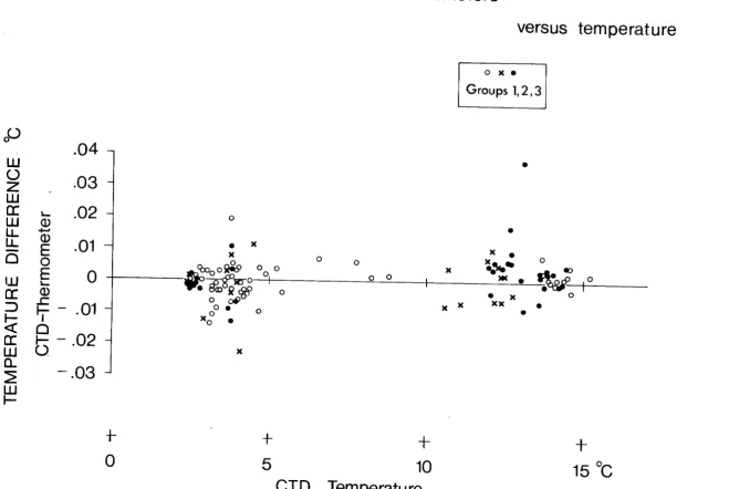
(b) Temperature
A plot of the difference between uncorrected CTD temperatures and
reversing thermometer values showed a difference of approximately
0.015°C near 15°C and 0.030°C near 3 C (CTD colder). Experience suggests
that this represents a CTD calibration shift which has occurred
during road/air shipment of the instrument or d u r i n g installation
aboard ship.* After adjustment of the temperature sensor calibration
(T = . 030+. OOOZ
i
.995
x
RA¥TEMP ) the difference b e t w e e n corrected CTD
temperature and reversing thermometer values was calculated and is
shown in figure 2.
No drift is discernable b e t w e e n first and last
stations and in the deep water rms differences a r e close to i.005°C,
the reading error of the thermometer.
On cruise 81 the fast
therm-istor was not installed and because subsequent experience has shown
that it introduces irrecoverable errors (Pollard, private
communi-cation) lOS intends to discontinue its use.
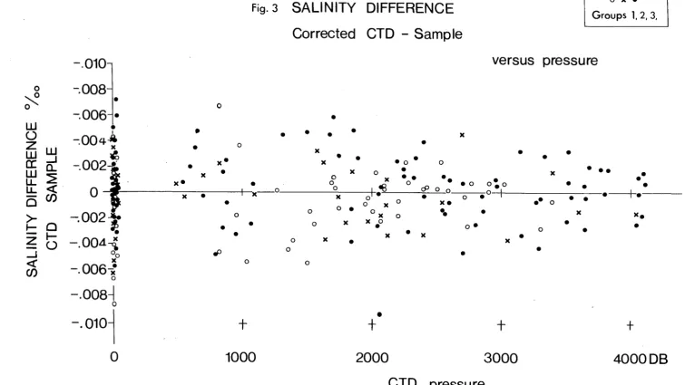
(c) Conductivity/Salinity
From the salinity of the sample, determined o n b o a r d usually within
2+8 hours, and from the corrected pressure and t e m p e r a t u r e of the CTD
the in-situ conductivity of the sample was c a l c u l a t e d (employing
algorithms supplied b y N.P. Fofonoff at ¥HOl). T h e ratio
of sample
conductivity (Cg) to CTD conductivity C was formed, and plotted versus
pressure.
Close examination of the data revealed that it fell into
three homogeneous groups which are identified in t a b l e 1. Within
each group of stations the conductivity ratio was a function only of
pressure and temperature, so that
Cs = CCR (1 + « T + ftp)
C
'
A least squares determination of these quantities yielded
- 5 Or^-1 a
r,
ot = ^5.0x10"^ "C"
p = - 7 . 0 x 1 0
db
CCR^
= 1.00094
CCRg
= 1.00105
CCR
= I
.OOIO9
From the raw CTD conductivity, corrected b y the f a c t o r CCR(
i + o
CT-*-Bp)
the CTD salinity was computed and the difference b e t w e e n it and the
sample salinity plotted in figure 3. The rms d i f f e r e n c e is s e e n to
be a function of pressure, about i.
005^o in the u p p e r 10OOdb
decreasing to ^ 0 0 2 ^ in the deep water; the latter figure is close
to the accuracy of the Autosal salinometer, the f o r m e r reflects the
variability resulting from heaving the instrument i n a gradient.
instruments.
Near the surface T=15,P=0 the term l+KT+^p has a value
.99925 : in the deep water T=2.5,p=4000 the factor h a s a value .99960.
This change is equivalent to a freshening of the surface with respect
to the deep water of .0^5%. The change in cell constant CCR during
the cruise was quite small corresponding to a salinity change of
only . 007^0.
COMPUTER PROCESSING OF CTD DATA
Data from the CTD was logged on the Hewlett Packard 2100 computer
employing software supplied by the Woods Hole Oceanographic
Institution (Tollios, Power and Ekstrand, unpublished manuscript
1 9 7 1 ) .
The data acquisition program permits simultaneous plotting
of temperature and salinity against pressure and one minute listing
of the data. Data logging is normally interrupted w h e n the lowering
is halted and restarted with winch restart: care must be exercised
to ensure that a depth range is not missed during a stop as height
changes of the instrument are common especially in strong current
shear. Although provisional analysis was conducted aboard Discovery
the in-situ calibration procedures were not completed until after
the cruise - so that a shore based computer was employed to handle
the data. lOS has access to the Science Research Council IBM 360/l95
computer at Rutherford Laboratory in Chilton: a processing system
G-EXEC has been implemented there b y Dr. K. Jeffrey and E.M. Gill and
has been modified for lOS use by Dr. R.T. Pollard and D.S. Collins
(both lOS).
Data processing is currently in batch and several programs are put
together to form a job.
The job may be submitted either on cards
or from disc files created from remote terminals.
The system is disc
based and capable of handling large data files - necessarily so as
deep CTD stations contain 100,000 data cycles. The computation path
will be described only in general terms commenting on special aspects
of the data handling; a description of the jobs is found in an
appendix but no detailed program listings are g i v e n .
The general character of the data processing is presented in
table 2. The steps outlined there are probably e s s e n t i a l to the task
of summarising CTD data in order to describe o c e a n i c properties on
both the medium and large scales.
Studies of micnrostructure may
require a somewhat different path, branching as e a r l y as stage 3 or
as late as stage 5, with a reduced pressure a v e r a g i n g interval.
Each stage of processing is commented on in the f o l l o w i n g paragraphs.
Stage 0. A method for matching time constants ± s described in
detail in Fofonoff et al {^91h). A procedure m o r e consistent with
lOS use of data is to slow the conductivity and p r e s s u r e probes to
match the slower response of the platinum r e s i s t a n c e thermometer.
This is achieved by employing a discrete r e p r e s e n t a t i o n of the
expression
t
C(t) = 1 C(t') exp ^
dt'
_ -00
where C and C are the slowed and observed conductivity respectively
and X is the time constant of the platinum resistance thermometer
(.2 to .25 seconds).
Stage 1 . Editing of data is achieved by e x a m i n i n g A the difference
between successive values of each variable in turn.
First the mean
A and rms cr are determined; those A for which | A — A ) > mO" are
excluded, where m is specified by the user, and m e a n A and rms C
recalculated.
Suspect data are identified as all
for which
|A-A'i >
and are listed and their location s t o r e d in an edit file.
Stage 2. After inspection of the lists g e n u i n e l y suspect data is
replaced by linearly interpolated values.
Stage 3. At present data cycles are sorted on tlxe pressure, which
implies that the heaving of the ship communicated t o the instrument
is ignored, and then averaged within an interval c h o s e n by the user
(2db centred on odd values).
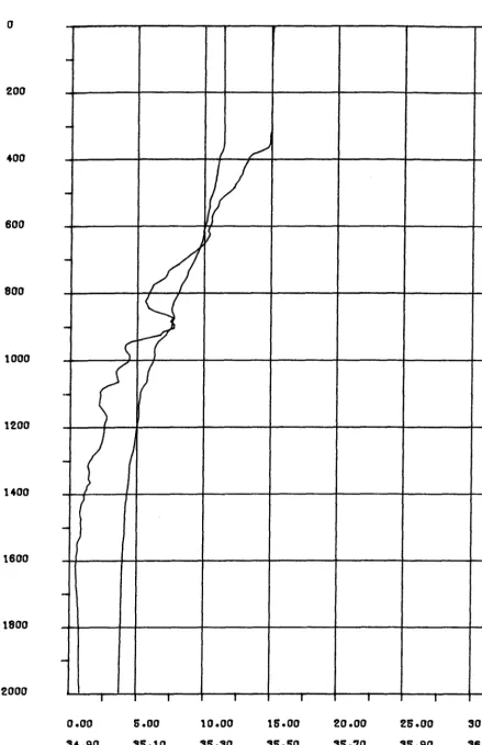
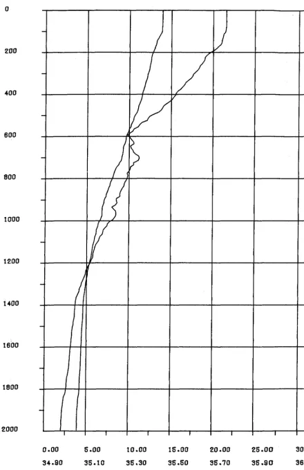
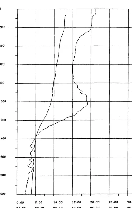
Stage 5. Standardised plots of temperature and salinity v e r s u s
pressure are drawn and for cruise 81 stations are reproduced in the
pages immediately after the appendix.
Page size o u t p u t is obtained
directly.
Stage 6.
Although raw data tapes are retained the first a r c h i v e d
4-1
-0
g
o
ElD
El
•W
t
f
i
m
o
o
o
U
Ph
CM
(D
r4
rO
(
t
i
H
k
5
6
7
EDIT BAD DATA
CONDENSE
FILL GAPS
PLOT
ARCHIVE
STATION LIST
(b) Identify suspect data,^ making enlries in an ed i t file.
Linearly interpolate snspect data: repeat sta^^e I (b)
Sort data on pressnre and average into 2db intervals:
list p,T,s.
Add any missing daia cycles.
Standard plot of T,s versus p.
Copy good file (p,T,s) to tape.
Compute standard hydi^of^rapliic parameters
^ etc...):
interpolate to standard pressures and list.
a;
Notes (l) ^ slow conductivity with a single-sided exponential filter of lia.l 1" width (). ;?3seconds
( 2 ) + suspect data identified as differing by several standard deviations from previous
good value.
data set of p,T,s is copied from disc to tape at t h i s stage and
stored for future use.
Stage 7. The following standaid oceanographic properties are
computed:-
potential temperature, potential d e n s i t y , dynamic height
anomaly, sound velocity, depth, specific volume a n o m a l y and
Brunt-Vaisala frequency. Linear interpolations are c a r r i e d out to levels
specified b y the user and lists generated. Lists for stations shown
in table 1 are presented in the final pages of t h i s report.
ACKNOWLEDGEMENTS
Mr. J. Moorey determined salinities and corrected thermometers,
the former with considerable skill and the latter with considerable
care; Mr. J. Smithers maintained the CTD at sea w i t h imperturbable
good humour; Dr. R.T. Pollard and Mr. D.S. Collins wrote most of the
software, enabling the writer to produce this data, report; and
Drs. W.J. Gould and J.C. Swallow assisted in the d a t a collection and
provided helpful advice and encouragement.
REFERENCES
BROWN, N and G. MORRISON. 1978 WHOl/Brown Conductivity, temperature
and depth microprofiler. WHOI-78-23
FOFONOFF, N.P., S.P. HAYES and R.C. MILLARD, Jr.
1 9 7 4
WHOl/Brown
CTD Hiicroprofiler; Methods of calibration a n d data handling.
Woods Hole Oceanographic Institution.
W H O I - 7 4 - 8 9 .
SWALLOW, J.C.
, W.J. GOULD and P.M. SAUNDERS. 1977 Evidence for a
poleward eastern boundary current in the N. Atlantic Ocean.
International Council for the exploration of the sea.
FIND MTAPEP448
MAKE
¥PRDI09291B¥
EXEC PCTDCL
Calibrate
0000001
CYCS , ,
C T D 1 , - . 0 0 0 0 5 , - . 0 0 0 0 0 0 0 7 , 0 . , 0 . , 0 - , . 1 0 0 7 , 1 0 0 . , . 0 3 , . 0 0 0 4 9 9 5 , . 0 0 1 0 0 0 9 4
VARS
,2,3,4
FIND ¥PRDI09291B¥
MAKE PHYSFILE,,,3,1
30000
EXEC PDECIM
Match, time constants
0
CYCS,,
DECI,16
SLO¥,I6,8
VARS,1,3
COPY
VARS,2
FIND PHYSFILE
MAKE ¥PRDI09291B¥
stage 1
Compute salinity and identify suspect data
EXEC POCEAN
0
CYCS,,
COPY
VARS,1,3
SAL1
VARS,P,1,G,2,T,3
FIND WPRDI09291B¥
MAKE PHYSFILE
,,,h,8000
EXEC PCOPYA
1
VARS,-COPY,,
FIND PHYSFILE
MAKE
WPRDI09291B¥
EXEC PSKTCH
0
CYCS,,
GROUP,
20
VARS,-FINP WRDI09291B¥
EXEC PCHECK
01
CYCS,,
ERRA,0.001
,8.0
VARS,-FIND ¥PRDI09291B¥
MAKE ¥PMSEDITFILA
Salinity
G r o u p sketch, of data
Create suspect data f i l e for |^
MAKE PHYSFILE,,,],
8000
EXEC PINTRP
0
LINEAR,-FIND PHYSFILE
MAKE ¥PRDIj2(9291B¥
EXEC PCHECK
01
CYCS,,
E R R A ,
. 0 . 0 0 1 , 8 . 0
VARS,-FIND
WPRDI09291B¥
MAKE WPMSEDITFILA
Linearly interpolate absent data
Create suspect data file again
stage 3
Condense data to 2db averages
EXEC PCOPYA
1
VARS,_
COPY,,
FIND WRDI09291B¥
M A K E
WPRDI09291B¥
EXEC PGFILE
0
FIND
¥PRDI09291B¥
MAKE TEMPFILE,,,3,8000
EXEC GS0RT3
00000000000000002000PRES
FIND TEMPFILE
MAKE ¥ORKFILE, , , 3 , 8j6j6j6
EXEC GPFILE
0
FIND ¥ORKFILE
MAKE PHYSFILE,,,3,8000
EXEC PAVRGE
0
SCIN,1,0.,2.0
VARS,-FIND PHYSFILE
MAKE ¥PRDI09291B¥
EXEC PLSTVR
0
CYCS,,
VARS,-FIND ¥PRDI09291B¥
File management
Sort data on pressure
Average data at 2db intervals
List 2db values
FIND ¥PRDI09291B¥
MAKE P H Y S F I L E , , , 3 , 2 2 #
EXEC PINTRP
Interpolates absent data (including new data cycle)
0
LINEAR,-FIND PHYSFILE
MAKE ¥PRDI09291B¥
EXEC PUSRIO
Changes pressure on 1st data cycle to 1.0
0
OVARS,-OTTDO
SUBROUTINE USERIO(INDISK,lODISK,INPOS,INVARS,IOFLDS,NSTART,NSTOP
& , ICON, NIC ,
FCON,
NFC ,
BUPA,
BUFB , SUMMIN, SUMMIO ,
ABSIN,
ABSIO ,
& INRECS,lORECS,INRECL,lORECL,NUM¥RD,INFLDS,RETREC)
DIMENSION INPOS(INVARS),ICON(19),FCON(19),BUFA(NUMWRD),
& BUFB
(NUMWRD) , SUMMIN
( NUMWRD ) , SUMMIO (
NUMWRD ) ,
ABSIN ( NUMWRD ) ,
& ABSIO (NUMWRD),RETREC (NUMWRD)
IORECS=INRECS
NUMDAT=1)2i
CALL INDATA(INDISK,1,1,NUMDAT,BUFA,
& RETREC,NDUMMY,INFLDS,INRECS,INRECL)
BUFA(I)=1.0
CALL OTDATA(INDISK,1,1,NUMDAT,BUFA,
& RETREC,NDUMMY,INFLDS,INRECS,INRECL)
RETURN
END
FIND ¥PRDI09291B¥
MAKE ¥RPDI09291B¥
EXEC PLSTVR
List 2db values
0
CYCS,,
VARS
FIND ¥PRDI09291B¥
stage 5
Standard plot of T,s versus p
EXEC PLOTXYjRLSP
0
CYCS,,
P L O T , 4 5 0 , 7 0 0 , 3 3 0 . 2 , 5 0 8 . 0
XAXIS,2,50.8,25.4
YAXIS,2,50.8,25.4
YVAR,PRES,0.
,2000.,h,200
XVAR,TEMP,0.
,32.5,1,5.0,
,,,,,1
XVAR,SAL.POF.
,34.9,36.2,1,0.2,
,,,,,1
FIND ¥PRDI09291B¥
Note; To make A4 size output, a scaling factor of 0.4 is employed
at the output stage.
Stage 6
Archives 2db data from disc file to tape
EXEC PTAPEP
0
FIND WPRDI09291B¥
MAKE •WPRDI0929
1B¥,ARCH,TAPE
VARS,P,1,T,2,S,3
SIGT
VARS,T,2,S,3
S I G P , 1 0 # .
VARS,P,1,T,2,S,3
DYNHT,0,0
VARS,P,1,T,2,8,3
SKDV
VARS,P,1,T,2,S,3
DEPTH,0.0
VARS,P,1,T,2,S,3
FIND WPRDI09291BW
MAKE PHYSFILE,,,9,2200
EXEC PFETCH
Interpolate quantities to standard pressure values
000002
CYCS,,
VARS,-SEARCH,PRES
LEVS , 10, 20,
, 50, 7
5,1
, 1 2
5 ,1
, 2
, 700, 800,900 ,1000
LEVS , 100,1 200,1 300,1 40jZ(, 1 500,1 600,1700,1800,1900, 2 0 0 0
LEVS,2200,2400,2600,2800,3000,3200,3400,3^00,3800,4000
FIND PHYSFILE
M A K E
¥PRDI09291B¥
EXEC P O C E A N
Calculate further oceanographic properties
0
CYCS,,
COPY
VARS,_
SVAN
VARS,P,1,T,2,S,3
BVFR
VARS,P,1,T,2,S,3
FIND ¥PRDI09291B¥
M A K E PHYSFILE,,,11,100
EXEC PTIMES
0
CYCS,,
COPY,-NE¥VAR,LNGITUDE,DEGREES,-999.,-23.908,0.0
FIND PHYSFILE
M A K E ¥PRDI09291B¥
EXEC PLSTDC
List data
1 1
( 1 HI//i+0X,'DISCOVERY 8l S T A T I O N 9 2 9 1 *
/ / l O X
'
P - D B
T - D E G C
S-0/00
POTEMP
SIGMAT
SIG1000'
'
DYNHT-M SNDV-M/S DEPTH-M
SVANOM
B V F R - C Y / H R ' / / / )
(1IX, F8.0,2F9.3,4F9.3,F9. 1
,F7.0,F11.6, F 9 . 3 )
CYCS,,
VARS,
FIND ¥ P R D I 0 9 2 9 1 B ¥
F i g . i
PRESSURE DIFFERENCE
Corrected CTD - Thermometer
(P and U)
versus pressure
GQ
Q
LU
U
z
LU
CC
LU
LL
Ll_
Q
UJ
DC
D
CO
CO
LU
DC
"D
c
CO
CO
<u
0)
E
0
E
(D
I—
1
Q
I
-20 n
10
0
—10
-a. o
- 2 0
0
O
o
o
- H
1000
o
°o
o o o
o
o
o
1 o
0 0 0
vo —
o
o
o
o °
°
o
o
o
o
o
3000
CTD Pressure
4
-3000
o O
HI
o
z
LU
DC
LU
U_
U_
Q
HI
DC
=)
DC
LU
CL
CD
4—"CD
E
o
E
0)
§
.04 n
.03
.02
.01 H
0
.01 H
.02
.03
O
Q
O
O
of"-5C"0—^
Groups 1,2,3
o O
m
f
0
+
+
5
10
CTD Temperature
[image:22.842.65.725.73.515.2]HI
ii
t Q
^
O
<
(/)
- . 0 1 0
. 0 0 8
. 0 0 6
-(
. 0 0 4 *
Fig. 3 SALINITY DIFFERENCE
Corrected CTD - Sample
•
o
Groups 1, 2, 3
versus pressure
X
o
I
o
o*
Q
I ^6
cP O
• •
•
:
X
X
• O O , o
•O
O—t—
X •
o •
•• O • •
X,
#
+
1000
+
2000
3000
CTD pressure
+
[image:23.843.50.805.50.475.2]200
400
600
800
1000
1200
1400
1600
1800
2 0 0 0
T
0.00
34.90
— r
5.00
35.10
— r
10.00
35.30
T
15.00
35.50
Fig
4-— r
20.00
35.70
— r
25.00
35.90
30.00
36.10
TEMP
[image:24.604.33.472.98.777.2]6AL.F0F.
zoo
400
600
800
1000
1200
1400
1600
1800
2000
0.00
34.90
5.00
35.10
10.00
35.30
15.00
35.50
Fig 5
20.00
35.70
2 5 . 0 0
3 5 . 9 0
30.00
36.10
TEMP
SflL.FOF.
[image:25.599.26.467.74.755.2]ZOO
400
600
800
1000
1200
1400
1600
1800
2000
0 . 0 0
34.90
5.00
35.10
10.00
35.30
15.00
35.50
Fig
6
2 0 . 0 0
35.70
25.00
35.90
30.00
36.10
TEMP
6AL.F0F.
PRES
2 0 0
400
600
800
1000
1200
1400
1600
1800
2000
0.00
34.30
5.00
35.10
10.00
35.30
15.00
35.50
Fdg 7
20.00
35.70
25.00
35.90
3 0 . 0 0
36.10
TEMP
6AL.F0F.
2 0 0
400
600
800
1000
1200
1400
1600
1800
2000
i
/
/
<
/
/
/
1
\
/
X
/
i
/
\
0 . 0 0
34.90
5.00
35.10
10.00
35.30
15.00
35.50
2 0 . 0 0
3 5 . 7 0
2 5 . 0 0
3 5 . 9 0
30.00
36.10
Figure 8
PLOTXY
PM8 DISCOVERY 81 STATION 9342 41 29N 28 21N
TEMP
8AL.F0F.
PRE8
5.00
15.00
35.50
34.90
35.10
10.00
35.30
2 0 . 0 0
35.70
2 5 . 0 0
3 5 . 9 0
30.00
36.10
TEMP
6AL.F0F.
Fig 9
[image:29.598.42.464.81.784.2]2 0 0
400
600
800
1000
1200
1400
1600
1800
2000
1
1
!
1
}
j / f
0.00
34.90
5.00
35.10
10.00
35.30
15.00
35.50
20.00
35.70
2 5 . 0 0
3 5 . 9 0
30.00
36.10
PLOTXY
Fig 10
PM6 DISCOVERY 81 STATION 9344 41 19N 27 29W
TEMP
SfiL.FOF,
[image:30.602.32.465.99.776.2]PRES
200
400
600
800
1000
1200
1400
1600
1800
2000
0 . 0 0
34.90
5.00
35.10
10.00
35.30
15.00
35.50
20.00
35.70
25.00
35.90
30.00
36.10
TEMP
8AL.F0F.
Fig 1 1
[image:31.597.34.494.92.776.2]ZOO
400
600
800
1000
1200
1400
1600
1800
2 0 0 0
0 . 0 0
34.90
5.00
35.10
10.00
35.30
15.00
35.50
20.00
35.70
25.00
35.90
30.00
36.10
TEMP
SflL.FOF-Fig
1 2
PRES
200
400
600
800
1000
1200
1400
1600
1800
2 0 0 0
0.00
34.90
5.00
35.10
10.00
35.30
15.00
35.50
F i ^ 13
20.00
35.70
2 5 . 0 0
3 5 . 9 0
30.00
36.10
TEMP
SfiL.FOF.
200
400
600
800
1000
1200
1400
1600
1800
2 0 0 0
J
/
-11
-- <
k
-//
1
'
1
1
1
1
1
1
0.00
34.90
5.00
35.10
10.00
35.30
15.00
35.50
20.00
35.70
2 5 . 0 0
3 5 . 9 0
30.00
36.10
TEMP
SflL.FOF.
PLOTXY
Fig 14
[image:34.598.27.468.100.768.2]PRES
200
400
600
800
1000
1200
1400
1600
1800
2000
/
J
'i
//
1)
0 . 0 0
34.90
5.00
35.10
10.00
35.30
15.00
35.50
Fig> 1 5
20.00
35.70
2 5 . 0 0
3 5 . 9 0
30.00
36.10
TEMP
8 A L . F 0 F .
200
400
600
800
1000
1200
1400
1600
1800
2000
0 . 0 0
34.90
5.00
35.10
10.00
35.30
15.00
35.50
Fig- 16
2 0 . 0 0
35.70
2 5 . 0 0
3 5 . 9 0
30.00
36.10
TEMP
SflL.FOF.
PRES
200
400
6 0 0
800
1000
1200
1400
1600
1800
2 0 0 0
J
i
J
1
\
/
1
K
(1
PLOTXY
0.00
5.00
10.00
15.00
20.00
2 5 . 0 0
34.90
35.10
35.30
35.50
35.70
3 5 . 9 0
Pig 17
PMS DISCOVERY 81 STATION 9398 41 06N 23 SOW
30.00
36.10
TEMP
SAL.FOF
200
400
600
800
1000
1200
1400
1600
1800
2000
0 . 0 0
34.90
T
5.00
35.10
— r
10.00
35.30
T
15.00
35.50
Pig 1%
— r
2 0 . 0 0
35.70
T
2 5 . 0 0
3 5 . 9 0
30.00
36.10
TEMP
SflL.FOF.
PRES
200
400
600
800
1000
1200
1400
1600
1800
2 0 0 0
0.00
34.90
5.00
35.10
10.00
35.30
15.00
35.50
Pig 19
20.00
35.70
2 5 . 0 0
3 5 . 9 0
30.00
36.10
TEMP
SflL.FOF.
200
400
600
800
1000
1200
1400
1600
1800
2000
0.00
34.90
5.00
35.10
10.00
3 5 . 3 0
15.00
35.50
Fig 20
20.00
3 5 . 7 0
2 5 . 0 0
3 5 . 9 0
30.00
36.10
TEMP
GAL.FOF.
[image:40.599.32.467.90.775.2]PRES
200
400
600
800
1000
1200
1400
1600
1800
2000
0.00
34.90
5.00
35.10
10.00
35.30
15.00
35.50
Fig 21
20.00
35.70
2 5 . 0 0
3 5 . 9 0
30.00
36.10
TEMP
SflL.FOF.
[image:41.597.31.470.95.776.2]200
400
600
800
1000
1200
1400
1600
1800
2000
7
0.00
34.90
5.00
35.10
10.00
35.30
15.00
3 5 . 5 0
P i g
20.00
35.70
2 5 . 0 0
3 5 . 9 0
30.00
36.10
TEMP
6AL.F0F.
PRE6
2 0 0
400
600
8 0 0
1000
1200
1400
1600
1800
2000
1
1
J
f
(
/
%
PLOTXY
0.00
5.00
10.00
15.00
20.00
2 5 . 0 0
30.00
34.30
35.10
35.30
35.50
35.70
3 5 . 9 0
3 6 . 1 0
Pig 23
PUS DISCOVERY 81 STATION 9395 41 24N 2 0 39W
0 7 J A N 8 0
TEMP
2 0 0
400
600
800
1000
1200
1400
1600
1800
2 0 0 0
0.00
34.90
5.00
35.10
10.00
35.30
15.00
35.50
Fig 24
20.00
35.70
25.00
35.90
30.00
36.10
TEMP
SflL.FOF.
[image:44.602.30.469.96.773.2]PRES
0.00
34.90
5.00
35.10
10.00
35.30
15.00
35.50
Fig 25
20.00
35.70
2 5 . 0 0
3 5 . 9 0
30.00
36.10
TEMP
8AL.F0F.
[image:45.597.42.461.97.772.2]200
400
600
800
1000
1200
1400
1600
1800
2 0 0 0
0.00
34.90
5.00
35.10
10.00
35.30
15.00
35.50
Fig
20.00
35.70
2 5 . 0 0
3 5 . 9 0
3 0 . 0 0
36.10
TEMP
6AL.F0F.
[image:46.602.24.468.98.767.2]PRE6
200
400
600
800
1000
1200
1400
1600
1800
2000
\
1
1
f
j y
j y
0 . 0 0
34.90
5.00
35.10
10.00
35.30
15.00
35.50
2 0 . 0 0
35.70
2 5 . 0 0
3 5 . 9 0
Pig 27
PLOTXY
PMS DISCOVERY 81 STATION 9393 41 36N 18 31H
30.00
36.10
TEMP
SflL.FOF.
ZOO
400
600
800
1000
1200
1400
1600
1800
2 0 0 0
J
1
1
I
. . ./
0.00
34.90
5.00
35.10
10.00
35.30
15.00
35.50
Pig 28
20.00
35.70
2 5 . 0 0
35.90
30.00
36.10
TEMP
SAL.FOF.
PKE6
200
600
0.00
34.90
5.00
35.10
10.00
35.30
15.00
35.50
F i K 28
20.00
35.70
2 5 . 0 0
3 5 . 9 0
30.00
36.10
TEMf
S A L . F 3 F ,
ZOO
400
600
800
1000
1200
1400
1600
1800
2000
)
1/
0.00
34.90
5.00
35.10
10.00
35.30
15.00
35.50
20.00
35.70
PLOTXY
Fig 3 0
PMS DISCOVERY 81 STATION 9406 41 45N 16 53W
25.00
35.90
30.00
36.10
TEMP
SAL.FOF.
[image:50.604.40.467.96.774.2]PRES
200
400
6 0 0
800
1000
1200
1400
1600
1800
2000
0.00
34.90
5.00
35.10
10.00
35.30
15.00
35.50
Fig 31
20.00
35.70
2 5 . 0 0
3 5 . 9 0
30.00
3 6 . 1 0
TEMP
6 A L . F 0 F .
[image:51.599.25.480.103.777.2]200
400
600
800
1000
1200
1400
1600
1800
2000
15.00
35.50
10.00
35.10
35.30
34.90
2 0 . 0 0
35.70
2 5 . 0 0
3 5 . 9 0
30.00
36.10
TEMP
SflL.FOF.
Fig 32
[image:52.604.38.469.93.769.2]PRES
0 . 0 0
34.90
5.00
35.10
10.00
35.30
15.00
35.50
Fig 3:
2 0 . 0 0
35.70
25.00
35.90
30.00
36.10
TEMP
SAL.FOF.
[image:53.601.36.472.106.778.2]200
400
600
800
1000
1200
1400
1600
1800
2000
/
I
\
<
1
t
/
1
1
1
1
0.00
34.90
5.00
35.10
10.00
35.30
15.00
35.50
20.00
35.70
PLOTXY
Fig 34
PM8 DISCOVERY 81 STATION 9389 41 53N 14 40H
25.00
35.90
30.00
36.10
TEMP
SAL.FOF.
[image:54.608.35.468.79.774.2]PRES
200
400
600
800
1000
1200
1400
1600
1800
2000
— r
0.00
3 4 . 9 0
— r
5 . 0 0
3 5 . 1 0
— r
1 0 . 0 0
3 5 . 3 0
— r
15.00
3 5 . 5 0
Fig 35
T
20.00
3 5 . 7 0
1_