Value at risk Predictions of Precious Metals with Long Memory Volatility Models

(1)

Munich Personal RePEc Archive

Value-at-risk Predictions of Precious

Metals with Long Memory Volatility

Models

Demiralay, Sercan and Ulusoy, Veysel

Faculty of Commercial Sciences, Yeditepe University, Faculty of

Commercial Sciences, Yeditepe University

27 January 2014

(2)

Value-at-risk Predictions of Precious Metals with Long Memory Volatility Models

Sercan Demiralaya,*, Veysel Ulusoya

a

Faculty of Commercial Sciences, Yeditepe University, Istanbul, Turkey

Abstract

In this paper, we investigate the value-at-risk predictions of four major precious metals (gold, silver, platinum, and palladium) with long memory volatility models, namely FIGARCH, FIAPARCH and HYGARCH, under

normal and student-t innovations’ distributions. For these analyses, we consider both long and short trading

positions. Overall, our results reveal that long memory volatility models under student-t distribution perform well in forecasting a one-day-ahead VaR for both long and short positions. In addition, we find that FIAPARCH model with student-t distribution, which jointly captures long memory and asymmetry, as well as fat-tails, outperforms other models in VaR forecasting. Our results have potential implications for portfolio managers, producers, and policy makers.

JEL classification: G17, C53, C58

Keywords: Long memory, value-at-risk, volatility modeling, precious metals prices

1. Introduction

Recently, stock markets have experienced unanticipated declines in returns and excessive volatility. Investors have lower diversification benefits from equity investments as correlations between global equity markets rise, especially in times of high volatility. Hence, financial market participants gravitate towards alternative asset classes to attain higher returns, diversify their portfolios and hedge against increased uncertainty in the equity markets. Commodities, such as major energy products and precious metals, are used as diversification and hedging tools as they have lower correlations with stocks. For this reason, modeling and forecasting volatility of commodity prices are of great interest to researchers, investors, portfolio managers and policymakers.

The empirical studies point out some stylized facts in the behavior of commodity prices, such as asymmetry, fat tails and long memory. Sophisticated volatility models that capture these characteristics, are found to produce more accurate volatility estimates and outperform other models in terms of forecasting performances. In order to analyze these features, fractionally integrated and/or asymmetric Generalized Autoregressive Conditional Heteroscedastic (GARCH)-class models are widely employed in the literature.

Accurate volatility estimates are also crucial for risk management. Empirical studies on commodity market risks frequently consider value-at-risk (VaR) approach based on GARCH-type models. VaR is commonly used among researchers and practitioners to measure the possible maximum amount of loss for an asset portfolio over a given period of time within a fixed confidence level.

A wealth of literature focuses on examining the volatility dynamics and/or the VaR predictions of oil and other energy prices (Giot and Laurent, 2003; Sadorsky, 2006; Cheong, 2009; Aloui and Mabrouk, 2010; Kang and Yoon, 2013), whereas related studies on precious metals are very limited. Many studies have shown that adding

precious metals in an equity portfolio considerably improves the portfolio performance.1 Precious metals are also

largely used in industries, such as electronics, jewelry and medicine. Hence, investigating precious metals from a risk management perspective is beneficial not only for portfolio managers but also for manufacturers.

In this paper, we investigate the value-at-risk (VaR) estimations of four precious metals (gold, silver, platinum and palladium) traded in the London Bullion Market and the London Platinum & Palladium Market, with long

*

Corresponding author. Tel: +90 216 578 0968

E-mail adresses: [email protected] (S. Demiralay), [email protected] (V. Ulusoy)

1

(3)

memory models, namely FIGARCH, FIAPARCH and HYGARCH. We use daily fixing spot prices from January, 4 1993 to November, 29 2013 and apply normal and student-t distributions to assess the overall performance. We evaluate in-sample and out-of-sample performances of the models at the 1% and 5% tails in the case of both long and short trading positions. In this regard, this study addresses a number of research questions. First, we investigate the volatility persistence in precious metals. Second, we examine the existence of asymmetric responses of precious metals volatility to the positive and negative news. Third, we analyze whether the long memory volatility models provide good forecasting performances of VaR if we jointly capture long memory, asymmetry and fat-tails in the precious metals volatility.

The remainder of the paper is as follows. Section 2 presents the literature review. Section 3 and 4 describes the methodology and preliminary data analysis. In section 5, we document the empirical results and discuss the findings. Section 6 concludes.

2. Literature Review

As pointed out by Arouri et al. (2012), empirical studies on precious metals can be divided into two lines of research. The first line focuses on the macroeconomic determinants of precious metals. In this respect, Ciner (2001) finds no stable long run relationship between the prices of gold and silver. This situation is attributed to the separate demand and supply forces and economic uses of the gold and silver markets. Therefore, these markets should be considered as separated markets. Christie-David et al. (2000) study on the responses of gold and silver future prices to monthly macroeconomic news releases using intraday data and report that both metals respond strongly to the release of capacity utilization. Gold responds strongly to the release of the CPI. The unemployment rate, gross domestic product and the PPI also have significant effects on gold. For silver, the authors document strong responses only to the release of the unemployment rate. In a related study, Batten et al. (2010) examine the macroeconomic determinants (business cycle, monetary environment and financial market sentiment) of four precious metals volatility. They indicate that gold volatility responds only to monetary variables. For platinum and palladium, both monetary and financial variables such as volatility on the S&P 500 are important, implying that these two metals are more likely to act as a financial instrument than gold. They also find that silver volatility responds neither to monetary nor financial market variables. Overall, their results show that precious metals are too distinct to be considered as a single asset class or represented by a single index.

The second line of research is devoted to the modeling and/or forecasting of precious metals volatility. Tully and Lucey (2007) employ asymmetric power GARCH (APARCH) model to both the cash and future prices of gold in two crisis period (1987 and 2001) and document that the model provides the most adequate description for the data. Baur (2012) investigates asymmetric volatility in the gold market conducting GJR-GARCH model and provide evidence of inverted asymmetric reaction to positive and negative shocks, i.e. positive shocks raise the volatility by more than negative shocks. Arouri et al. (2012) analyze long memory and structural breaks in returns and volatility of precious metal commodities (gold, silver, platinum and palladium) and report that conditional volatility of precious metals is better explained by long memory than by structural breaks. Furthermore, they assert that an ARFIMA-FIGARCH model, which captures dual long memory both in the returns and volatility, provides better out-of-sample forecast accuracy than other volatility models. In the multivariate context, Hammoudeh et al. (2010) use VARMA-GARCH model to analyze precious metals-exchange rate volatility transmission. They provide evidence of weak volatility transmissions among precious metals and volatility sensitivity of precious metals to the exchange rate volatility. Computing hedge ratios and optimal portfolio weights, they also stress the role of gold as a hedge against exchange rate risk.

The recent empirical studies have centered upon how to improve forecasts of VaR with volatility models in commodity markets. The generalized autoregressive conditional heteroscedastic (GARCH)-class models have been widely used in the finance literature to produce reliable predictions of VaR. Broadly speaking, these studies

have also shown that distributional assumptions are very vital. In the context of precious metals’ market,

(4)

innovations yield fewer violations. Cheng and Hung (2011) investigate the VaR forecasting performance of skewed generalized-t (SGT) distribution in the petroleum and metal markets. Based on the unconditional and conditional coverage tests, their results suggest that GARCH (1, 1) model with SGT distribution produces the most reliable VaR predictions. Aloui and Mabrouk (2010) compute VaR and expected shortfalls (ESFs) for some major crude oil and gas commodities by combining long memory volatility models with three alternative

innovation’s distributions. They find that fractionally integrated asymmetric power GARCH (FIAPARCH) model with skewed student-t distribution performs well in predicting a one-day-ahead VaR for both long and short trading positions. Chikili et al. (2014) analyze VaR predictions of four major commodities (crude oil, natural gas, gold, silver) with several GARCH-type models and posit that FIAPARCH model under student-t distribution is found to be the best suited for predicting VaR. The above empirical findings are consistent with the results of the studies in the related field, asserting that the models, which jointly capture some stylized facts in the commodity prices behavior, produce superior predictions of VaR.

As indicated earlier, this paper focuses on VaR forecasting ability of the three competing long memory volatility models (FIGARCH, FIAPARCH and HYGARCH) with normal and student-t distributions in the context of precious metals. As the first step, we examine volatility estimates of the models, capturing the aforementioned

stylized facts in the commodity prices’ behavior. In the sequel, we compare the models according to the in-sample and out-of-in-sample performances in estimating market risk of precious metals for both long and short trading positions.

3. Methodology

3.1. Detection of Long Memory

It is a well known fact that many financial time series are highly persistent, implying that an unforeseeable shock to the variable has long lasting impacts. In this case, autocorrelations of the absolute and squared returns of the time series exhibit very slow decay.

To detect the long memory behavior in returns and volatility of precious metals, we apply three well known long

memory tests, namely the Lo’s modified rescaled range (R/S) analysis (1991), the log-periodogram regression

(GPH) of Geweke and Porter-Hudak (1983) and the Gaussian semi-parametric (GSP) method of Robinson and Henry (1999).

3.1.1. Lo’s R/S Statistic

The Rescaled Range (R/S) statistic was originally proposed by Hurst (1951) and later modified by Lo (1991). Lo (1991) remarked that the original statistic is not robust to short range dependence. Thus, Lo (1991) modified the R/S statistic as follows,





₁





1

1 1

1

max min

ˆ ( )

k k

j _{k T} j

k T _j _j

T T

y y y y

q

Q

   _   _

     _    _    



฀ (1) where 1 1/ T i i

y T y





and



ˆ

_T

( )

q

represents the square root of the Newey-West estimate of the long –run

variance with bandwidth q.

3.1.2. GPH Test

Geweke and Porter-Hudak (1983) proposed a semi-parametric approach to test for long memory, using the following regression,

 

2





(5)

where w_j 2



j/T, j=1,2,…n; ηjis the residual term and wj denotes Fourier frequencies. I(wj) represents the

periodogram of a time series rt and defined as

 

2

1 1 2 j T w t j t t

I w r e

T



 





(3)

3.1.3. GSP Test

The Gaussian semi-parametric estimation proposed by Robinson and Henry (1999) is based on the Whittle approximation maximum likelihood estimation. GSP estimator can be written as;

 

ˆ _{arg min}

GSP d

d  R d (4)

 

2

 

1 1

1 2

log log

m m

d

j j j

j j

d

R d I

m    m  

 

 _ _









where m is the bandwidth, which increases with the sample size T. I(λj) denotes the periodogram and λj=2πj/T.

3.2. Long Memory Volatility Models

3.2.1. The Fractionally Integrated GARCH (FIGARCH) Model

Baillie et al. (1996) extended the standard GARCH model by incorporating a fractionally integrated process, I(d)

and suggested that FIGARCH model can distinguish between short and long memory in the conditional variance

process. The FIGARCH (p,d,q) model can be expressed as follows:

   



 

2 ₁ ₁ d 2 2

t L L L t L t

    _    _   (5)

where L denotes backshift or lag operator. ω, β, φ and d are the parameters of the model to be estimated and

0≤d≤1. The FIGARCH (p,d,q) model nests the IGARCH (p,q) model for d=1 and GARCH (p,q) model for d=0.

3.2.2. The Fractionally Integrated Asymmetric Power ARCH (FIAPARCH) Model

Tse (1998) proposed the FIAPARCH model by introducing fractional integration to the asymmetric power

GARCH model of Ding et al. (1993). The FIAPARCH (p,d,q) model can be written as follows:

 

1



 

1

 









1 1 1 1 d

t L L L L t t

 

 _   _ _   _  

 _  _  _ _   (6)

where δ, γ, φ, d and β are the model parameters and 0≤d≤1. δ denotes a Box-Cox transformation of the

conditional standard deviation and it is estimated within the model rather than being imposed by the researcher. γ

represents the asymmetry parameter, i.e. when γ>0, negative shocks have bigger impact on volatility than

positive shocks and vice versa. The FIAPARCH model nests the FIGARCH model for γ=0 and δ=2.

3.2.3. Hyperbolic GARCH (HYGARCH) Model

Davidson (2004) extended the conditional variance of the FIGARCH model by incorporating weights to its difference operator. The HYGARCH model can be defined as follows:

 

1



 

1

 









2 2

1 1 1 1 1 d

t L L L L t

   _  _     _  _  _   _  (7)

(6)

3.3 Value-at-Risk (VaR) Concept

VaRs are computed on a 1-day 99% and 95% confidence level basis, implying that the losses are more than the

reported VaR of a portfolio in only 1% and 5% of the cases.2 We also calculate VaRs for both long (buy) and

short (sell) trading positions. In the case of long positions, investors incur the risk of a loss when the traded asset price declines; hence we model the left tail of returns distributions. In the case of short positions, the risk of a loss occurs when the asset price rises; accordingly we model the right tail of the distribution.

The estimated VaRs for long and short trading positions under normal distribution are expressed as follows:

ˆ ˆ

long t t

VaR  z_ (8)

1

ˆ ˆ

short t t

VaR  z__

where zα and z1-α denote the left and right quantile at α% of the normal distribution, respectively.



ˆ

tand



ˆ

t represent the estimated daily conditional mean and standard deviation of precious metals returns generated from the long memory volatility models.

The estimated VaRs for long and short trading positions under student-t distribution are computed as follows:

,

ˆ ˆ

long t v t

VaR  st_  (9)

1 ,

ˆ ˆ

short t v t

VaR  st_ 

where st,vand st1,vare the left and right quantiles at α% for the student-t distribution with v degrees of freedom.

In order to assess the statistical accuracy of the estimated VaRs, we employ two backtesting measures, namely the unconditional coverage test of Kupiec (1995) and the dynamic quantile test of Engle and Manganelli (2004). As a backtesting procedure, we compute the empirical failure rates for both long and short trading positions. The failure rate is the number of times returns exceed the forecasted VaR and should be equal to the designated level of VaR, if the VaR model is correctly specified.

Kupiec (1995) proposed a likelihood ratio statistic to test the null hypothesis that the failure rate is statistically equal to the expected one. The likelihood ratio statistic is as follows:













2 log N 1 T N 2 log N 1 T N

UC

LR       f  f  (10)

where N is the number of violations in the sample size T, f denotes the failure rate computed as N/T and α is the

pre-specified VaR level. Under the null hypothesis, LRUC is distributed as χ2

(1).

Engle and Manganelli (2004) introduced Dynamic Quantile (DQ) test to jointly examine whether the number of failures is equal to the expected one and the probability of violations is independent of all past information. The following sequence is defined as:

( )

t t t

Hit I r  VaR  (11)

where Hitt is an indicator function and θ=1-α denotes a given confidence level. The sequence takes the value

(1-θ) in the case that rt is less than the VaRt and (θ) otherwise.

2_{Portfolio managers usually focus on longer forecasting horizons. However, as evidenced by Christoffersen and Diebold}

(7)

Using an artificial regression, we test the independence of Hitt and regress it on a constant and the lagged Hitt-m

up to the lag m=5, as follows:

0 1 1 2 2 ... 5 5

t t t t t

Hit   Hit_  Hit_   Hit_  (12)

or

t t

Hit  X 

We test the null hypothesis, H0:β=0, indicating uncorrelated hits. Engle and Manganelli (2004) provided that

under the null hypothesis, the DQ test statistic is:

ˆ ˆ

(1 )

X X DQ  

 

 

 (13)

The asymptotic distribution of the test statistic is chi-squared with seven degrees of freedom, χ2(7).

4. Preliminary Data Analysis

In this paper, we consider daily PM fixing spot prices of four precious metals (gold, silver, platinum and palladium) traded in the London Bullion Market and the London Platinum & Palladium Market. All the prices are in US$/Troy ounce. The fixings are the globally published and accepted benchmark prices for precious metals trading. The time span is from January 4, 1993 to November 29, 2013, which is a highly volatile period covering the late 1990s global recession due to the Asian financial crisis and the recent global financial crisis. The last 1000 observations are used to conduct the out-of-sample analysis. For the forecasting procedure, we re-estimate

the model parameters in every 50 observations based on a rolling sample of the out-of-sample observations.3

The continuously compounded daily returns are calculated as:



1



100 ln /

t t t

R  P P_ (14)

where Rt is the return in percent and Pt and Pt-1 denotes the closing price on day t and t-1, respectively.

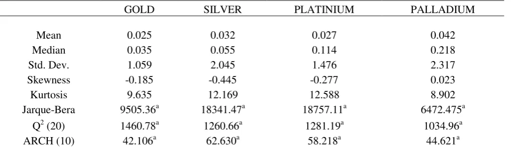
Descriptive statistics for the daily log returns of the precious metals are reported in Table 1. We find that the highest mean returns are for the palladium (0.042), lowest mean returns are for the gold (0.025) and the values of standard deviations range from 2.317 (palladium) to 1.059 (gold). Table 1 also demonstrates that all the precious

metals’ returns exhibit excess kurtosis which implies fatter tails than a normal distribution. Jarque-Bera (JB) test confirms the non-normal distribution of the return series, rejecting the null hypothesis of normality. Additionally, from the Ljung-Box tests employed to the squared returns, we can reject the null hypothesis of no serial correlation, hence the squared returns do not display white noise property. Based on the ARCH tests, ARCH

effects are present in the precious metals’ returns. For this reason, GARCH-class models are appropriate for modeling dynamic conditional volatility.

3

All the computations were performed with G@RCH 6.0 on the Ox package. We used the Quassi Maximum Likelihood

(8)

[image:8.595.46.559.81.229.2]

Table 1. Descriptive Statistics

GOLD SILVER PLATINIUM PALLADIUM

Mean 0.025 0.032 0.027 0.042

Median 0.035 0.055 0.114 0.218

Std. Dev. 1.059 2.045 1.476 2.317

Skewness -0.185 -0.445 -0.277 0.023

Kurtosis 9.635 12.169 12.588 8.902

Jarque-Bera 9505.36a 18341.47a 18757.11a 6472.475a

Q2 (20) 1460.78a 1260.66a 1281.19a 1034.96a

ARCH (10) 42.106a 62.630a 58.218a 44.621a

Notes: Q2(20) is the Ljung-Box Q-statistics of order 20 on the squared return series. ARCH (10) denotes ARCH Lagrange multiplier test

of order 10. (a) represents statistical significance at the 1% level.

Some preliminary tests are implemented to check for the existence of unit-roots and to test stationarity, before fitting the data. We apply two unit-root tests (Augmented Dickey Fuller, ADF; 1979 and Phillips-Perron, PP;

1988) and a stationary test (Kwiatkowski–Phillips–Schmidt–Shin, KPSS; 1992) to the return series. These three

tests differ in their null hypotheses. While the null hypothesis of ADF and PP tests imply the presence of a

unit-root, I (1) process, the KPSS test has the null hypothesis of stationarity, I (0) process. In table 2, we present the

results of these three tests. ADF and PP tests clearly reject the null hypothesis of a unit-root for all the precious metals at a 1% significance level. The statistics of KPSS tests indicate that all the return series are insignificant for the rejection of the null hypothesis of stationarity. Hence, the return series are stationary and convenient for further tests and models.

Table 2. Unit root and stationarity tests

ADF -71.859a -78.535a -70.259a -61.674a

PP -71.861a -78.535a -70.259a -61.574a

KPSS 0.131 0.066 0.062 0.085

Notes: MacKinnon's (1991) 1% critical value is −3.435 for the ADF and PP tests. The critical value for the KPSS test is 0.739 at the 1%

significance level. (a) represents statistical significance at the 1% level.

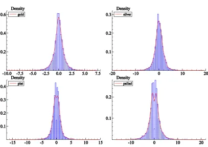
Descriptive graphs are given in Figures (1-4) to provide a visual representation. Figure 1 presents the time

evolution of daily precious metals’ returns and exhibits volatility clustering behavior, i.e. large (small) changes

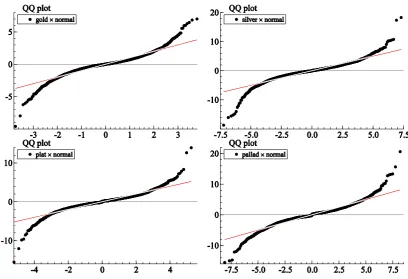
tend to be followed by large (small) changes. Figure 2 displays the histograms of the daily returns against normal distribution and reveals that all the daily returns have fat tails and leptokurtosis. The autocorrelation functions of the raw and squared returns are plotted in Figure 3. From this figure, it is evident that most autocorrelations are insignificant and stay inside the 95% confidence intervals for the raw returns. However, the autocorrelations of the squared returns are positive and statistically significant up to many lags. They also display hyperbolic and slow decay, suggesting a persistent behavior in the squared returns of the precious metals. In figure 4, we present the quantile-quantile (QQ) plots against the normal distribution. QQ-plots confirm the results of the histograms,

[image:8.595.41.554.430.494.2]

(9)

[image:9.595.75.483.403.690.2]

Figure1. Plots of precious metals daily returns

(10)

[image:10.595.84.483.69.342.2]

Figure 3. Autocorrelations of daily raw and squared precious metals returns

[image:10.595.74.483.387.666.2]

(11)

5. Empirical Results

5.1. Long Memory Test Results

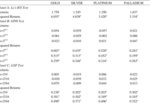
We utilize three long memory tests to the raw and squared returns of the precious metals.4 The results of the tests

are documented in Table 3. Panel A of Table 3 shows that Lo’s modified R/S statistics support the null

hypothesis of short memory in the returns, whereas the statistics indicate that long memory behavior exists in the volatility proxy, which is squared returns.

[image:11.595.52.553.266.611.2]

From Panel B and C of Table 3, we can clearly notice that both GPH and GSP tests do not reject the null hypothesis of no long-range dependence for the precious metals returns. For the squared return series, the results of the both tests provide evidence of long memory. Thereby, the results of long memory tests point out the suitability of GARCH-class models which capture long memory property in the volatility process.

Table 3. Long memory tests results

Panel A: Lo's R/S Test

Returns 1.758 1.245 1.290 1.627

Squared Returns 6.055a 4.838a 3.420a 3.334a

Panel B: GPH Test Returns

m=T0.5 0.054 -0.039 -0.057 0.021

m=T0.6 -0.061 -0.029 -0.002 0.086

m=T0.8 -0.023 -0.010 0.021 0.047

Squared Returns

m=T0.5 0.603a 0.435a 0.520a 0.281a

m=T0.6 0.515a 0.313a 0.452a 0.359a

m=T0.8 0.259a 0.246a 0.216a 0.263a

Panel C: GSP Test Returns

m=T/4 0.005 -0.019 0.006 0.022

m=T/16 -0.020 -0.039 0.032 0.025

m=T/64 0.070 -0.009 0.044 0.013

Squared Returns

m=T/4 0.238a 0.202a 0.203a 0.302a

m=T/16 0.381a 0.302a 0.349a 0.345a

m=T/64 0.498a 0.371a 0.406a 0.352a

Notes: The critical values of Lo’s modified R/S statistic is 2.098 at the 1% level, m represents the bandwidth for the GPH and GSP tests. (a) denotes statistical significance at the 1% level.

5.2. Estimation Results of GARCH-class Models

In tables 4-6, we present the estimation results of FIGARCH, FIAPARCH and HYGARCH models under normal

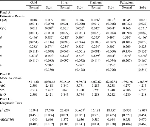
and student-t distributed innovations for all precious metals returns.5 The Panel A of Table 4 shows that the

estimates of the long memory parameter d are all positive and statistically significant at the 1% level, suggesting

4

It is well known that long memory tests are very sensitive to the selection of bandwith. Therefore, the GPH test was applied with different bandwidths: m=T0.5,m=T0.6 and m=T0.8. For the GSP test, it was estimated for diverse bandwidths: m=T/4, m=T/16, and m=T/64.

5

(12)

the rejection of d=0 (GARCH model) and d=1 (IGARCH model). This empirical result provides evidence of long memory in the volatility of precious metals returns. Under the student-t distribution, the tail parameters (v) are significantly different from zero, indicating the fat-tail phenomenon.

Examining the log-likelihood values and the lowest values of three information criterions (AIC, SIC and H-Q) in Panel B of Table 4, we find that the FIGARCH models with student-t distribution outperform those with normal

distribution. In addition, as residual diagnostic tests, we employ the Ljung-Box test up to 20th order serial

[image:12.595.47.551.246.671.2]

correlation in the squared residuals and the ARCH-LM test for the existence of ARCH effects in the residuals up to lags 10. Panel C documents the tests’ results and implies no serial correlations in the standardized squared residuals, except for one case. More importantly, ARCH (10) tests show no remaining ARCH effects in the residuals.

Table 4. FIGARCH Model Estimation Results

Gold Silver Platinum Palladium

Normal Std-t Normal Std-t Normal Std-t Normal Std-t

Panel A.

Estimation Results

C(M) 0.004 0.005 0.010 0.016 0.036b 0.038b 0.045 0.020

(0.011) (0.009) (0.021) (0.020) (0.017) (0.016) (0.032) (0.027)

C(V) 0.017 0.007b 0.061b 0.053b 0.042b 0.041a 0.166 0.231a

(0.011) (0.003) (0.027) (0.021) (0.020) (0.014) (0.090) (0.089)

d 0.446a 0.587a 0.518a 0.504a 0.555a 0.495a 0.510a 0.496a

(0.051) (0.116) (0.098) (0.096) (0.109) (0.087) (0.101) (0.078)

φ 0.282b 0.274a 0.254a 0.337a 0.274a 0.307a 0.269 0.223

(0.111) (0.049) (0.067) (0.061) (0.081) (0.060) (0.156) (0.132)

β 0.604a 0.756a 0.694a 0.738a 0.659a 0.641a 0.539a 0.465a

(0.119) (0.083) (0.092) (0.072) (0.114) (0.074) (0.207) (0.169)

υ 5.207a 5.648a 7.352a 6.187a

- (0.380) - (0.428) - (0.796) - (0.544)

Panel B.

Model Selection

L -5214.61 -5030.48 -8035.35 -7889.04 -6369.62 -6276.84 -7392.76 -7283.93

AIC 2.506 2.418 3.840 3.771 3.285 3.238 4.277 4.215

SIC 2.514 2.427 3.848 3.780 3.293 3.248 4.286 4.225

H-Q 2.509 2.421 3.843 3.774 3.288 3.242 4.280 4.218

Panel C.

Diagnostic Tests

Q2 (20) 17.941 27.690 27.407 30.677b 16.181 18.457 16.937 18.017

[0.459] [0.066] [0.071] [0.031] [0.579] [0.425] [0.527] [0.454]

ARCH(10) 1.040 1.646 1.372 1.656 0.580 0.664 0.951 0.970

[0.406] [0.102] [0.186] [0.141] [0.831] [0.758] [0.484] [0.467]

Notes: L denotes the log-likelihood. AIC, SIC and H-Q represents Akaike, Schwarz and Hannan-Quinn information criterions,

respectively. Q2_{(20) is the Ljung-Box test statistic for the remaining serial correlation for standardized squared residuals. ARCH (10) is}

the ARCH Lagrange Multiplier test at lag 10. (a) and (b) stand for 1% and 5% significance levels, respectively. Robust standard errors are in parentheses and the values in brackets are the p-values.

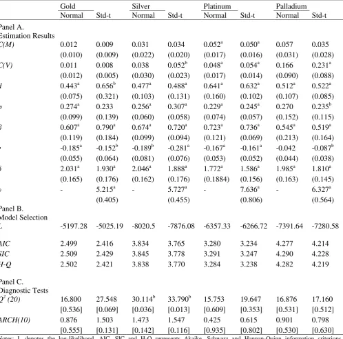
Estimation results for the FIAPARCH model with normal and student-t error distributions are reported in the

Panel A of Table 5. The fractional difference parameters, d are all positive and significant, consistent with

FIGARCH model results. The asymmetric news impact coefficients, γ are all negative and statistically

(13)

negative asymmetry coefficients imply that positive shocks have bigger impacts on conditional volatility than negative shocks of the same magnitude. This asymmetric effect can be attributed to the general perception of investors that upward price movements in precious metals (especially in gold and silver markets) are signals of uncertainty in equity markets and future unfavorable macroeconomic conditions. These bring higher volatility to

the precious metals markets. The tail parameters (v) of the FIAPARCH model with student-t distribution indicate

that the densities of the model’s standardized residuals have fat tails.

Panel B of Table 5 demonstrates that FIAPARCH models with student-t distribution give superior results, with regards to the maximum log-likelihood and minimum information criterions. Besides, based on the results in the Panel C, Q2 (20) tests fail to reject the null hypothesis of no serial correlation in the standardized squared

[image:13.595.50.549.247.738.2]

residuals, except for silver. For heteroscedasticity tests, ARCH (10) tests indicate no remaining ARCH effects.

Table 5. FIAPARCH Model Estimation Results

Panel A.

Estimation Results

C(M) 0.012 0.009 0.031 0.034 0.052a 0.050a 0.057 0.035

(0.010) (0.009) (0.022) (0.020) (0.017) (0.016) (0.031) (0.028)

C(V) 0.011 0.008 0.038 0.052b 0.048a 0.054a 0.166 0.231a

(0.012) (0.005) (0.030) (0.023) (0.017) (0.014) (0.090) (0.088)

d 0.443a 0.656b 0.477a 0.488a 0.641a 0.632a 0.512a 0.522a

(0.075) (0.321) (0.103) (0.131) (0.160) (0.102) (0.107) (0.085)

φ 0.274a 0.233 0.256a 0.307a 0.229a 0.245a 0.270 0.235b

(0.099) (0.139) (0.060) (0.058) (0.074) (0.057) (0.152) (0.115)

β 0.607a 0.790a 0.674a 0.720a 0.723a 0.736a 0.545a 0.519a

(0.119) (0.184) (0.099) (0.094) (0.121) (0.069) (0.213) (0.164)

γ -0.185a -0.152b -0.189b -0.281a -0.167a -0.161a -0.042 -0.087b

(0.055) (0.064) (0.081) (0.076) (0.053) (0.052) (0.044) (0.038)

δ 2.031a 1.930a 2.046a 1.888a 1.772a 1.586a 1.985a 1.810a

(0.165) (0.176) (0.162) (0.176) (0.1884) (0.156) (0.163) (0.145)

υ - 5.215a - 5.727a - 7.636a - 6.327a

(0.405) (0.455) (0.806) (0.564)

Panel B.

Model Selection

L -5197.28 -5025.19 -8020.5 -7876.08 -6357.33 -6266.72 -7391.64 -7280.58

AIC 2.499 2.416 3.834 3.765 3.280 3.234 4.277 4.214

SIC 2.509 2.429 3.845 3.778 3.291 3.247 4.290 4.228

H-Q 2.502 2.421 3.838 3.770 3.284 3.238 4.282 4.219

Panel C.

Diagnostic Tests

Q2 (20) 16.800 27.548 30.114b 33.790b 15.753 19.647 16.876 17.160

[0.536] [0.069] [0.036] [0.013] [0.609] [0.353] [0.531] [0.512]

ARCH(10) 0.876 1.503 1.473 1.547 0.425 0.615 0.901 0.798

[0.555] [0.131] [0.142] [0.116] [0.935] [0.802] [0.530] [0.630]

respectively. Q2_{(20) is the Ljung-Box test statistic for the remaining serial correlation for standardized squared residuals. ARCH (10) is}

the ARCH Lagrange Multiplier test at lag 10. (a) and (b) stand for 1% and 5% significance levels, respectively. Robust standard errors are

(14)

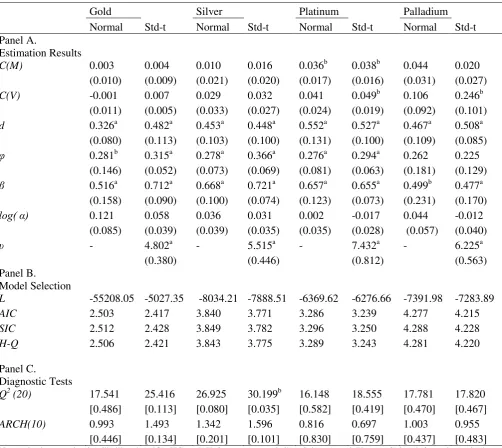
The Panel A of Table 6 documents the estimation results of HYGARCH models with normal and student-t

innovations’ distributions. The results reveal that the hyperbolic parameters log (α) are not statistically different

from zero, suggesting that the GARCH components are covariance stationary. The tail parameters (v) of student-t

distribution are all significant at the 1% level, referring to the fat-tails.

The Panel B of Table 6 provides evidence of HYGARCH models with student-t error distribution being a more

suitable model than those with normal distribution. Furthermore, as can be seen from the Panel C, Q2 (20) test

results show no serial correlation in the standardized squared residuals, excluding silver’s HYGARCH model

[image:14.595.48.551.230.678.2]

with student-t distribution. With the HYGARCH models, we fail to reject the null hypothesis of no remaining ARCH effects.

Table 6. HYGARCH Model Estimation Results

Panel A.

Estimation Results

C(M) 0.003 0.004 0.010 0.016 0.036b 0.038b 0.044 0.020

(0.010) (0.009) (0.021) (0.020) (0.017) (0.016) (0.031) (0.027)

C(V) -0.001 0.007 0.029 0.032 0.041 0.049b 0.106 0.246b

(0.011) (0.005) (0.033) (0.027) (0.024) (0.019) (0.092) (0.101)

d 0.326a 0.482a 0.453a 0.448a 0.552a 0.527a 0.467a 0.508a

(0.080) (0.113) (0.103) (0.100) (0.131) (0.100) (0.109) (0.085)

φ 0.281b 0.315a 0.278a 0.366a 0.276a 0.294a 0.262 0.225

(0.146) (0.052) (0.073) (0.069) (0.081) (0.063) (0.181) (0.129)

β 0.516a 0.712a 0.668a 0.721a 0.657a 0.655a 0.499b 0.477a

(0.158) (0.090) (0.100) (0.074) (0.123) (0.073) (0.231) (0.170)

log( α) 0.121 0.058 0.036 0.031 0.002 -0.017 0.044 -0.012

(0.085) (0.039) (0.039) (0.035) (0.035) (0.028) (0.057) (0.040)

υ - 4.802a - 5.515a - 7.432a - 6.225a

(0.380) (0.446) (0.812) (0.563)

Panel B.

Model Selection

L -55208.05 -5027.35 -8034.21 -7888.51 -6369.62 -6276.66 -7391.98 -7283.89

AIC 2.503 2.417 3.840 3.771 3.286 3.239 4.277 4.215

SIC 2.512 2.428 3.849 3.782 3.296 3.250 4.288 4.228

H-Q 2.506 2.421 3.843 3.775 3.289 3.243 4.281 4.220

Panel C.

Diagnostic Tests

Q2 (20) 17.541 25.416 26.925 30.199b 16.148 18.555 17.781 17.820

[0.486] [0.113] [0.080] [0.035] [0.582] [0.419] [0.470] [0.467]

ARCH(10) 0.993 1.493 1.342 1.596 0.816 0.697 1.003 0.955

[0.446] [0.134] [0.201] [0.101] [0.830] [0.759] [0.437] [0.483]

respectively. Q2 (20) is the Ljung-Box test statistic for the remaining serial correlation for standardized squared residuals. ARCH (10) is

the ARCH Lagrange Multiplier test at lag 10. (a) and (b) stand for 1% and 5% significance levels, respectively. Robust standard errors are

in parentheses and the values in brackets are the p-values.

Summarizing all, when we compare FIGARCH, FIAPARCH and HYGARCH models under the two innovations’

(15)

captures long memory behavior and asymmetry in the volatility of precious metals returns as well as fat-tails in the density of the standardized residuals.

5.3. Estimation Results of VaR Computations

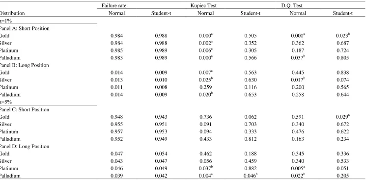
In Tables 7(a)-(c) and 8(a)-(c), we present the empirical results for the in-sample and out-of-sample VaR

computations, respectively, for the precious metals with a VaR level α; 1% and 5% for long trading positions and

99% and 95% for short trading positions.6 In these tables we report the results of empirical failure rates, Kupiec

and Dynamic Quantile tests. The failure rate indicates the percentage of positive (negative) returns larger (smaller) than the VaR prediction for short (long) trading position. The failure rate is equal to the pre-specified

VaR level if the VaR model is correctly specified. Moreover, for an adequate model, Kupiec’ LR and Dynamic

Quantile tests would not reject their null hypothesis, implying that the failure rate is equal to the pre-specified

VaR level and the exceptions are not serially correlated.

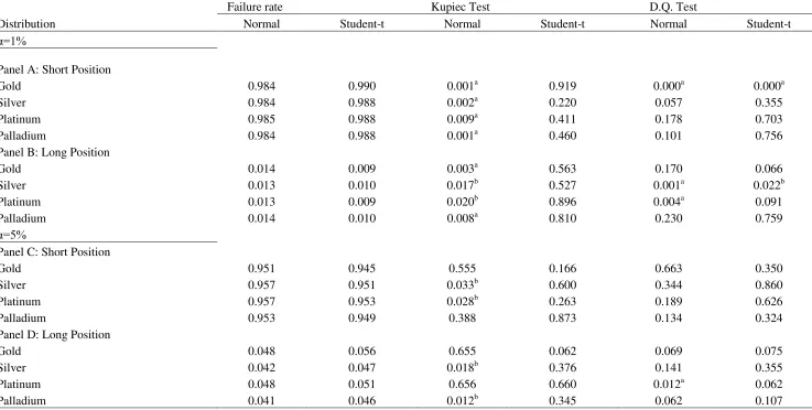
Tables 7(a)-(c) show that, overall, long memory volatility models with student-t innovations’ distribution perform

better than those with normal distribution for the in-sample VaR analyses. Out of 16 cases, the null hypothesis of

Kupiec’s LR test is rejected in 9, 12 and 10 cases for FIGARCH, FIAPARCH and HYGARCH models with

normally distributed innovations, respectively. Under student-t distribution, the Kupiec’s LR test is rejected in 1

case for FIGARCH model and none of the cases for FIAPARCH and HYGARCH models. Hence, we can draw a conclusion that the number of violations implied by normal distribution is greater than those under student-t distribution. In Tables 7(a)-(c), Dynamic Quantile test results reveal that, out of 16 cases, VaR violations are not independently distributed in 5 cases for the FIGARCH model and 4 cases for both the FIAPARCH and HYGARCH models with normally distributed innovations. Assuming student-t distribution, all the long memory volatility models pass the test at all confidence levels, except for 2 cases in each.

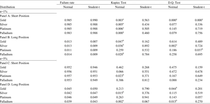
As suggested by Tang and Shieh (2006), the main contribution of VaR computation is its forecasting performance, providing insights for investors and financial institutions about the maximum amount of loss that

they will incur. Diamandis et al. (2011) also consider the out-of-sample VaR analysis as the “true” test. In this

regard, we present the one-day-ahead forecasting results of the long memory volatility models in Tables 8(a)-(c). To conduct the analysis, the last 1000 observations are used and we employed an iterative procedure by re-estimating every 50 observations in the out-of-sample period. Tables 8(a)-(c) indicate that long-memory models with normally distributed innovations have a poor forecasting performance, compared to those with student-t distribution. Out of 16 cases in each, Kupiec test results indicate that all of the models under normal distribution have 4 rejections. The models with student-t distribution perform better and yield fewer rejections; 2 rejections for both FIGARCH and HYGARCH models and 1 rejection for FIAPARCH model.

Based on the Dynamic-Quantile test results, the majority of the VaR violations are independently distributed. However, FIGARCH and FIAPARCH models under normal distribution have 3 rejections, followed by HYGARCH model with 1 rejection. Under student-t distribution, both FIGARCH and HYGARCH models have 1 rejection and FIAPARCH model has no rejection. Hence, FIAPARCH model with student-t distribution perform correctly in 100% of the cases for both long and short trading positions. In a nutshell, our VaR forecasting analyses clearly demonstrate that long memory volatility models under normal distribution have a very poor performance to model large positive and negative returns, compared to those with student-t distribution. Within the context of VaR, our results provide evidence of relevance and usefulness of realistic assumptions, such as long memory, asymmetry and fat tails. These assumptions give rise to a deeper understanding of investors, portfolio and risk managers about the uncertainty associated with the maximum amount of loss that they will incur.

6

(16)

Table 7(a). In sample VaR calculated by FIGARCH model

Failure rate Kupiec Test D.Q. Test

Distribution Normal Student-t Normal Student-t Normal Student-t

α=1%

Panel A: Short Position

Gold 0.984 0.988 0.000a 0.505 0.000a 0.023b

Silver 0.984 0.988 0.002a 0.352 0.362 0.687

Platinum 0.985 0.989 0.006a 0.305 0.187 0.724

Palladium 0.983 0.989 0.000a 0.566 0.037b 0.805

Panel B: Long Position

Gold 0.014 0.009 0.007a 0.563 0.445 0.838

Silver 0.013 0.010 0.025b 0.630 0.017b 0.074

Platinum 0.011 0.008 0.259 0.116 0.200 0.565

Palladium 0.014 0.009 0.020b 0.653 0.258 0.644

α=5%

Panel C: Short Position

Gold 0.948 0.943 0.736 0.062 0.591 0.029b

Silver 0.955 0.951 0.091 0.703 0.340 0.672

Platinum 0.957 0.953 0.094 0.333 0.476 0.622

Palladium 0.952 0.949 0.433 0.812 0.163 0.234

Panel D: Long Position

Gold 0.047 0.054 0.462 0.188 0.345 0.336

Silver 0.043 0.047 0.056 0.459 0.340 0.533

Platinum 0.046 0.049 0.037b 0.882 0.005a 0.051

Palladium 0.039 0.042 0.004a 0.046b 0.022b 0.205

Notes: D.Q. Test represents Dynamic Quantile test of Engle and Manganelli (2004). For Kupiec’s LR Test and D.Q. Test, the associated p-values are documented. (a) and (b) stand for 1% and 5%

[image:16.842.60.805.119.486.2]

(17)

Table 7(b). In sample VaR calculated by FIAPARCH model

α=1%

Gold 0.984 0.990 0.001a 0.919 0.000a 0.000a

Silver 0.984 0.988 0.002a 0.220 0.057 0.355

Platinum 0.985 0.988 0.009a 0.411 0.178 0.703

Palladium 0.984 0.988 0.001a 0.460 0.101 0.756

Gold 0.014 0.009 0.003a 0.563 0.170 0.066

Silver 0.013 0.010 0.017b 0.527 0.001a 0.022b

Platinum 0.013 0.009 0.020b 0.896 0.004a 0.091

Palladium 0.014 0.010 0.008a 0.810 0.230 0.759

α=5%

Gold 0.951 0.945 0.555 0.166 0.663 0.350

Silver 0.957 0.951 0.033b 0.600 0.344 0.860

Platinum 0.957 0.953 0.028b 0.263 0.189 0.626

Palladium 0.953 0.949 0.388 0.873 0.134 0.324

Gold 0.048 0.056 0.655 0.062 0.069 0.075

Silver 0.042 0.047 0.018b 0.376 0.141 0.355

Platinum 0.048 0.051 0.656 0.660 0.012a 0.062

Palladium 0.041 0.046 0.012b 0.345 0.062 0.107

[image:17.842.60.797.75.447.2]

(18)

Table 7(c). In sample VaR calculated by HYGARCH model

α=1%

Gold 0.985 0.990 0.003a 0.563 0.000a 0.000a

Silver 0.985 0.988 0.005a 0.434 0.077 0.336

Platinum 0.985 0.988 0.006a 0.505 0.145 0.719

Palladium 0.983 0.988 0.000a 0.460 0.079 0.756

Gold 0.013 0.007 0.047b 0.162 0.614 0.489

Silver 0.013 0.009 0.036b 0.892 0.002a 0.724

Platinum 0.011 0.009 0.259 0.532 0.186 0.037b

Palladium 0.014 0.009 0.020b 0.784 0.258 0.695

α=5%

Gold 0.952 0.946 0.462 0.268 0.475 0.159

Silver 0.956 0.951 0.066 0.551 0.472 0.678

Platinum 0.957 0.953 0.023b 0.371 0.167 0.649

Palladium 0.953 0.949 0.306 0.812 0.088 0.234

Gold 0.045 0.050 0.213 0.790 0.044b 0.201

Silver 0.042 0.047 0.015b 0.376 0.115 0.519

Platinum 0.046 0.049 0.263 0.941 0.143 0.057

Palladium 0.039 0.043 0.002a 0.067 0.015b 0.270

[image:18.842.58.797.72.437.2]

(19)

Table 8(a). Out-of-sample VaR calculated by FIGARCH model

α=1%

Gold 0.985 0.995 0.138 0.048b 0.816 0.523

Silver 0.986 0.990 0.230 1.000 0.503 0.997

Platinum 0.991 0.992 0.746 0.510 0.997 0.990

Palladium 0.986 0.993 0.230 0.313 0.506 0.002a

Gold 0.024 0.014 0.000a 0.230 0.026b 0.896

Silver 0.021 0.015 0.002a 0.138 0.000a 0.213

Platinum 0.015 0.014 0.136 0.230 0.816 0.896

Palladium 0.024 0.013 0.000a 0.362 0.084 0.950

α=5%

Gold 0.954 0.949 0.556 0.884 0.649 0.898

Silver 0.957 0.955 0.298 0.460 0.265 0.454

Platinum 0.969 0.967 0.003a 0.008a 0.028b 0.074

Palladium 0.952 0.951 0.770 0.884 0.392 0.397

Gold 0.056 0.062 0.392 0.092 0.639 0.400

Silver 0.048 0.050 0.770 1.000 0.116 0.149

Platinum 0.051 0.056 0.884 0.730 0.896 0.725

Palladium 0.050 0.056 1.000 0.392 0.567 0.640

[image:19.842.59.799.72.437.2]

(20)

Table 8(b). Out-of-sample VaR calculated by FIAPARCH model

α=1%

Gold 0.986 0.989 0.230 0.754 0.896 0.993

Silver 0.987 0.992 0.362 0.510 0.950 0.990

Platinum 0.991 0.992 0.746 0.732 0.997 0.995

Palladium 0.986 0.993 0.230 0.313 0.002a 0.506

Gold 0.023 0.016 0.000a 0.079 0.028b 0.474

Silver 0.020 0.016 0.005a 0.079 0.000a 0.093

Platinum 0.018 0.015 0.062 0.138 0.380 0.497

Palladium 0.024 0.013 0.000a 0.362 0.084 0.465

α=5%

Gold 0.954 0.945 0.556 0.474 0.462 0.722

Silver 0.958 0.951 0.233 0.884 0.523 0.755

Platinum 0.968 0.966 0.005a 0.130 0.072 0.164

Palladium 0.953 0.951 0.660 0.884 0.499 0.484

Gold 0.055 0.073 0.474 0.001a 0.666 0.071

Silver 0.047 0.053 0.660 0.666 0.096 0.082

Platinum 0.053 0.059 0.666 0.203 0.688 0.621

Palladium 0.051 0.055 0.884 0.474 0.601 0.621

[image:20.842.56.797.71.437.2]

(21)

Table 8(c). Out-of-sample VaR calculated by HYGARCH model

α=1%

Gold 0.989 0.996 0.754 0.030b 0.993 0.166

Silver 0.988 0.992 0.537 0.510 0.980 0.990

Platinum 0.991 0.992 0.746 0.510 0.997 0.990

Palladium 0.986 0.993 0.230 0.313 0.506 0.002a

Gold 0.020 0.011 0.005a 0.754 0.226 0.993

Silver 0.018 0.015 0.022b 0.138 0.251 0.213

Platinum 0.015 0.014 0.138 0.230 0.816 0.896

Palladium 0.024 0.013 0.000a 0.362 0.084 0.950

α=5%

Gold 0.959 0.953 0.178 0.660 0.330 0.425

Silver 0.959 0.955 0.178 0.460 0.189 0.454

Platinum 0.968 0.966 0.005a 0.013b 0.047 0.164

Palladium 0.952 0.951 0.770 0.884 0.392 0.397

Gold 0.050 0.054 1.000 0.566 0.814 0.562

Silver 0.046 0.049 0.556 0.884 0.046b 0.134

Platinum 0.051 0.056 0.884 0.392 0.896 0.725

Palladium 0.050 0.058 1.000 0.257 0.567 0.581

[image:21.842.59.798.72.437.2]

(22)

6. Conclusion

This paper analyzes the value-at-risk (VaR) predictions of major precious metals with long memory volatility models under normal and student-t distributions. Our main results are threefold. First, carrying out the three widely employed long memory tests, we document long-range dependence in the volatility process of precious metals. Second, according to the model selection criterions, the FIAPARCH model with student-t distribution is found to be the best suited for estimating the conditional variance of the precious metals. The estimation results of the FIAPARCH model also show that positive shocks have bigger impacts on conditional volatility of precious metals than negative shocks of the same magnitude. Finally, in overall, long memory volatility models perform well in both in-sample and out-of-sample VaR analyses for long and short trading positions. However, the FIAPARCH model under student-t distribution outperforms other models in predicting a one-day-ahead VaR of

the precious metals, in regard to Kupiec’s LR and Dynamic Quantile tests. In general terms, our results point out

the usefulness of the sophisticated volatility models which consider some stylized facts, such as long memory, asymmetry and fat-tails, to quantify and predict market risk of precious metals in the context of VaR.

For a further research, the use of intra-day data might be beneficial to produce more reliable measures of the

market risk for traders. In addition, other types of innovations’ distributions, such as α-stable distributions, can be considered. Moreover, longer forecasting time horizons might be employed to provide more information about market risk of precious metals for portfolio managers.

References

Aloui, C., & Mabrouk, S. (2010). Value-at-risk estimations of energy commodities via long-memory, asymmetry

and fat-tailed GARCH models. Energy Policy, 38(5), 2326-2339.

Arouri, M. E. H., Hammoudeh, S., Lahiani, A., & Nguyen, D. K. (2012). Long memory and structural breaks in

modeling the return and volatility dynamics of precious metals. The Quarterly Review of Economics and

Finance, 52(2), 207-218.

Baillie, R. T., Bollerslev, T., & Mikkelsen, H. O. (1996). Fractionally integrated generalized autoregressive

conditional heteroskedasticity. Journal of econometrics, 74(1), 3-30.

Batten, J. A., Ciner, C., & Lucey, B. M. (2010). The macroeconomic determinants of volatility in precious metals

markets. Resources Policy, 35(2), 65-71.

Baur, G. D. (2012). Asymmetric volatility in the gold market. The Journal of Alternative Investments, 14(4),

26-38.

Cheong, C. W. (2009). Modeling and forecasting crude oil markets using ARCH-type models. Energy

policy, 37(6), 2346-2355.

Chkili, W., Hammoudeh, S., & Nguyen, D. K. (2014). Volatility forecasting and risk management for commodity

(23)

Christie–David, R., Chaudhry, M., & Koch, T. W. (2000). Do macroeconomics news releases affect gold and

silver prices?. Journal of Economics and Business, 52(5), 405-421.

Christoffersen, P. F., & Diebold, F. X. (2000). How relevant is volatility forecasting for financial risk

management?. Review of Economics and Statistics, 82(1), 12-22.

Ciner, C. (2001). On the long run relationship between gold and silver prices A note. Global Finance

Journal, 12(2), 299-303.

Conover, C. M., Jensen, G. R., Johnson, R. R., & Mercer, J. M. (2009). Can precious metals make your portfolio

shine?. Journal of Investing, 18(1), 75-86.

Davidson, J. (2004). Moment and memory properties of linear conditional heteroscedasticity models, and a new

model. Journal of Business & Economic Statistics, 22(1).

Diamandis, P. F., Drakos, A. A., Kouretas, G. P., & Zarangas, L. (2011). Value-at-risk for long and short trading

positions: Evidence from developed and emerging equity markets. International Review of Financial

Analysis, 20(3), 165-176.

Dickey, D. A., & Fuller, W. A. (1979). Distribution of the estimators for autoregressive time series with a unit

root. Journal of the American statistical association, 74(366a), 427-431.

Ding, Z., Granger, C. W., & Engle, R. F. (1993). A long memory property of stock market returns and a new

model. Journal of empirical finance, 1(1), 83-106.

Engle, R. F., & Manganelli, S. (2004). CAViaR: Conditional autoregressive value at risk by regression

quantiles. Journal of Business & Economic Statistics,22(4), 367-381.

Geweke, J., & Porter‐Hudak, S. (1983). The estimation and application of long memory time series

models. Journal of time series analysis, 4(4), 221-238.

Giot, P., & Laurent, S. (2003). Market risk in commodity markets: a VaR approach. Energy Economics, 25(5),

(24)

Hammoudeh, S. M., Yuan, Y., McAleer, M., & Thompson, M. A. (2010). Precious metals–exchange rate

volatility transmissions and hedging strategies. International Review of Economics & Finance, 19(4), 633-647.

Hammoudeh, S., Malik, F., & McAleer, M. (2011). Risk management of precious metals. The Quarterly Review

of Economics and Finance, 51(4), 435-441.

Hurst, H. E. (1951). Long-term storage capacity of reservoirs. Trans. Amer. Soc. Civil Eng., 116, 770-808.

Jensen, G. R., Johnson, R. R., & Mercer, J. M. (2002). Tactical asset allocation and commodity futures. The

Journal of Portfolio Management, 28(4), 100-111.

Kang, S. H., & Yoon, S. M. (2012). Modelling and forecasting the volatility of petroleum futures prices. Energy

Economics.

Kupiec, P. H. (1995). Techniques for verifying the accuracy of risk measurement models. THE J. OF

DERIVATIVES, 3(2).

Kwiatkowski, D., Phillips, P. C., Schmidt, P., & Shin, Y. (1992). Testing the null hypothesis of stationarity against the alternative of a unit root: How sure are we that economic time series have a unit root?. Journal of econometrics, 54(1), 159-178.

Lo, A.W. (1991). Long term memory in stock market prices. Econometrica59, 1279-1313

Phillips, P. C., & Perron, P. (1988). Testing for a unit root in time series regression. Biometrika, 75(2), 335-346.

Robinson, P. M., & Henry, M. (1999). Long and short memory conditional heteroskedasticity in estimating the

memory parameter of levels. Econometric theory, 15(3), 299-336.

Sadorsky, P. (2006). Modeling and forecasting petroleum futures volatility.Energy Economics, 28(4), 467-488.

Tang, T. L., & Shieh, S. J. (2006). Long memory in stock index futures markets: A value-at-risk

(25)

Tse, Y. K. (1998). The conditional heteroscedasticity of the yen-dollar exchange rate. Journal of Applied Econometrics, 13(1), 49-55.

Tully, E., & Lucey, B. M. (2007). A power GARCH examination of the gold market. Research in International