Extractive Summarization using Continuous Vector Space Models
Mikael K˚ageb¨ack, Olof Mogren, Nina Tahmasebi, Devdatt Dubhashi
Computer Science & Engineering Chalmers University of Technology
SE-412 96, G¨oteborg
{kageback, mogren, ninat, dubhashi}@chalmers.se
Abstract
Automatic summarization can help users extract the most important pieces of infor-mation from the vast amount of text digi-tized into electronic form everyday. Cen-tral to automatic summarization is the no-tion of similarity between sentences in text. In this paper we propose the use of continuous vector representations for se-mantically aware representations of sen-tences as a basis for measuring similar-ity. We evaluate different compositions for sentence representation on a standard dataset using the ROUGE evaluation mea-sures. Our experiments show that the eval-uated methods improve the performance of a state-of-the-art summarization frame-work and strongly indicate the benefits of continuous word vector representations for automatic summarization.
1 Introduction
The goal of summarization is to capture the im-portant information contained in large volumes of text, and present it in a brief, representative, and consistent summary. A well written summary can significantly reduce the amount of work needed to digest large amounts of text on a given topic. The creation of summaries is currently a task best han-dled by humans. However, with the explosion of available textual data, it is no longer financially possible, or feasible, to produce all types of sum-maries by hand. This is especially true if the sub-ject matter has a narrow base of interest, either due to the number of potential readers or the duration during which it is of general interest. A summary describing the events of World War II might for instance be justified to create manually, while a summary of all reviews and comments regarding a certain version of Windows might not. In such cases, automatic summarization is a way forward.
In this paper we introduce a novel application of continuous vector representations to the prob-lem of multi-document summarization. We evalu-ate different compositions for producing sentence representations based on two different word em-beddings on a standard dataset using the ROUGE evaluation measures. Our experiments show that the evaluated methods improve the performance of a state-of-the-art summarization framework which strongly indicate the benefits of continuous word vector representations for this tasks.
2 Summarization
There are two major types of automatic summa-rization techniques, extractive and abstractive. Ex-tractive summarizationsystems create summaries using representative sentences chosen from the in-put whileabstractive summarization creates new sentences and is generally considered a more dif-ficult problem.
Figure 1: Illustration of Extractive Multi-Document Summarization.
For this paper we consider extractive multi-document summarization, that is, sentences are chosen for inclusion in a summary from a set of documents D. Typically, extractive summariza-tion techniques can be divided into two compo-nents, the summarization framework and the sim-ilarity measures used to compare sentences. Next
we present the algorithm used for the framework and in Sec. 2.2 we discuss a typical sentence sim-ilarity measure, later to be used as a baseline. 2.1 Submodular Optimization
Lin and Bilmes (2011) formulated the problem of extractive summarization as an optimization prob-lem using monotone nondecreasing submodular set functions. A submodular function F on the set of sentencesV satisfies the following property: for anyA⊆B ⊆V\{v},F(A+{v})−F(A)≥
F(B+{v})−F(B)wherev∈V. This is called the diminishing returns property and captures the intuition that adding a sentence to a small set of sentences (i.e., summary) makes a greater contri-bution than adding a sentence to a larger set. The aim is then to find a summary that maximizes di-versity of the sentences and the coverage of the in-put text. This objective function can be formulated as follows:
F(S) =L(S) +λR(S)
whereS is the summary,L(S)is the coverage of the input text,R(S)is a diversity reward function. The λis a trade-off coefficient that allows us to define the importance of coverage versus diversity of the summary. In general, this kind of optimiza-tion problem is NP-hard, however, if the objective function is submodular there is a fast scalable al-gorithm that returns an approximation with a guar-antee. In the work of Lin and Bilmes (2011) a sim-ple submodular function is chosen:
L(S) =X
i∈V
min{X
j∈S
Sim(i, j), αX
j∈V
Sim(i, j)}
(1) The first argument measures similarity between sentence i and the summary S, while the sec-ond argument measures similarity between sen-tencei and the rest of the input V. Sim(i, j) is the similarity between sentence iand sentence j
and0 ≤α ≤1is a threshold coefficient. The di-versity reward functionR(S)can be found in (Lin and Bilmes, 2011).
2.2 Traditional Similarity Measure
Central to most extractive summarization sys-tems is the use of sentence similarity measures (Sim(i, j) in Eq. 1). Lin and Bilmes measure similarity between sentences by representing each sentence using tf-idf (Salton and McGill, 1986) vectors and measuring the cosine angle between
vectors. Each sentence is represented by a word vectorw = (w1, . . . , wN)whereN is the size of the vocabulary. Weightswki correspond to the tf-idf value of wordkin the sentencei. The weights
Sim(i, j)used in theLfunction in Eq. 1 are found using the following similarity measure.
Sim(i, j) =
P
w∈itfw,i×tfw,j ×idf 2 w r P
w∈itf 2
w,i×idf2wr P w∈jtf
2
w,j×idf2w (2) where tfw,i and tfw,j are the number of occur-rences of w in sentence iand j, and idfw is the inverse document frequency (idf) ofw.
In order to have a high similarity between sen-tences using the above measure, two sensen-tences must have an overlap of highly scoredtf-idfwords. The overlap must be exact to count towards the similarity, e.g, the terms The US President and Barack Obamain different sentences will not add towards the similarity of the sentences. To cap-ture deeper similarity, in this paper we will inves-tigate the use of continuous vector representations for measuring similarity between sentences. In the next sections we will describe the basics needed for creating continuous vector representations and methods used to create sentence representations that can be used to measure sentence similarity. 3 Background on Deep Learning
Deep learning(Hinton et al., 2006; Bengio, 2009) is a modern interpretation of artificial neural net-works (ANN), with an emphasis on deep network architectures. Deep learning can be used for chal-lenging problems like image and speech recogni-tion (Krizhevsky et al., 2012; Graves et al., 2013), as well as language modeling (Mikolov et al., 2010), and in all cases, able to achieve state-of-the-art results.
Inspired by the brain, ANNs use a neuron-like construction as their primary computational unit. The behavior of a neuron is entirely controlled by its input weights. Hence, the weights are where the information learned by the neuron is stored. More precisely the output of a neuron is computed as the weighted sum of its inputs, and squeezed into the interval[0,1]using a sigmoid function:
yi=g(θTi x) (3)
x1
x2
x3
x4
y3 Hidden
layer Input
[image:3.595.91.288.62.205.2]layer Outputlayer
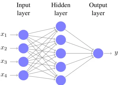
Figure 2: FFNN with four input neurons, one hid-den layer, and 1 output neuron. This type of ar-chitecture is appropriate for binary classification of some datax ∈ R4, however depending on the complexity of the input, the number and size of the hidden layers should be scaled accordingly.
whereθi are the weights associated with neuroni andxis the input. Here the sigmoid function (g) is chosen to be the logistic function, but it may also be modeled using other sigmoid shaped functions, e.g. the hyperbolic tangent function.
The neurons can be organized in many differ-ent ways. In some architectures, loops are permit-ted. These are referred to asrecurrent neural net-works. However, all networks considered here are non-cyclic topologies. In the rest of this section we discuss a few general architectures in more de-tail, which will later be employed in the evaluated models.
3.1 Feed Forward Neural Network
A feed forward neural network (FFNN) (Haykin, 2009) is a type of ANN where the neurons are structured in layers, and only connections to sub-sequent layers are allowed, see Fig 2. The algo-rithm is similar to logistic regression using non-linear terms. However, it does not rely on the user to choose the non-linear terms needed to fit the data, making it more adaptable to changing datasets. The first layer in a FFNN is called the input layer, the last layer is called the output layer, and the interim layers are called hidden layers. The hidden layers are optional but necessary to fit complex patterns.
Training is achieved by minimizing the network error (E). HowE is defined differs between dif-ferent network architectures, but is in general a differentiable function of the produced output and
x1
x2
x3
x4
x′
1
x′
2
x′
3
x′
4 Coding
layer Input
layer Reconstructionlayer
Figure 3: The figure shows an auto-encoder that compresses four dimensional data into a two di-mensional code. This is achieved by using a bot-tleneck layer, referred to as a coding layer.
the expected output. In order to minimize this function the gradient ∂E
∂Θ first needs to be calcu-lated, where Θ is a matrix of all parameters, or weights, in the network. This is achieved using backpropagation (Rumelhart et al., 1986). Sec-ondly, these gradients are used to minimizeE us-ing e.g. gradient descent. The result of this pro-cesses is a set of weights that enables the network to do the desired input-output mapping, as defined by the training data.
3.2 Auto-Encoder
An auto-encoder (AE) (Hinton and Salakhutdinov, 2006), see Fig. 3, is a type of FFNN with a topol-ogy designed for dimensionality reduction. The input and the output layers in an AE are identical, and there is at least one hidden bottleneck layer that is referred to as the coding layer. The net-work is trained to reconstruct the input data, and if it succeeds this implies that all information in the data is necessarily contained in the compressed representation of the coding layer.
A shallow AE, i.e. an AE with no extra hid-den layers, will produce a similar code as princi-pal component analysis. However, if more layers are added, before and after the coding layer, non-linear manifolds can be found. This enables the network to compress complex data, with minimal loss of information.
3.3 Recursive Neural Network
[image:3.595.317.513.66.188.2]x1
x2
x3
y
Root layer Input
[image:4.595.93.247.63.208.2]layer
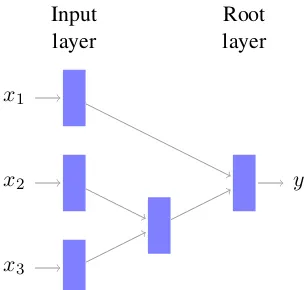
Figure 4: The recursive neural network architec-ture makes it possible to handle variable length in-put data. By using the same dimensionality for all layers, arbitrary binary tree structures can be re-cursively processed.
binary parse tree produced by linguistic parsing of a sentence. This is achieved by enforcing weight constraints across all nodes and restricting the out-put of each node to have the same dimensionality as its children.
The input data is placed in the leaf nodes of the tree, and the structure of this tree is used to guide the recursion up to the root node. A com-pressed representation is calculated recursively at each non-terminal node in the tree, using the same weight matrix at each node. More precisely, the following formulas can be used:
zp =θTp[xl;xr] (5a)
yp =g(zp) (5b)
where yp is the computed parent state of neuron
p, and zp the induced field for the same neuron.
[xl;xr]is the concatenation of the state belonging to the right and left sibling nodes. This process re-sults in a fixed length representation for hierarchi-cal data of arbitrary length. Training of the model is done using backpropagation through structure, introduced by Goller and Kuchler (1996).
4 Word Embeddings
Continuous distributed vector representation of words, also referred to as word embeddings, was first introduced by Bengio et al. (2003). A word embedding is a continuous vector representation that captures semantic and syntactic information about a word. These representations can be used to unveil dimensions of similarity between words, e.g. singular or plural.
4.1 Collobert & Weston
Collobert and Weston (2008) introduce an efficient method for computing word embeddings, in this work referred to asCW vectors. This is achieved firstly, by scoring a valid n-gram (x) and a cor-rupted n-gram (¯x) (where the center word has been randomly chosen), and secondly, by training the network to distinguish between these two n-grams. This is done by minimizing the hinge loss
max(0,1−s(x) +s(¯x)) (6)
wheresis the scoring function, i.e. the output of a FFNN that maps between the word embeddings of an n-gram to a real valued score. Both the pa-rameters of the scoring function and the word em-beddings are learned in parallel using backpropa-gation.
4.2 Continuous Skip-gram
A second method for computing word embeddings is the Continuous Skip-gram model, see Fig. 5, in-troduced by Mikolov et al. (2013a). This model is used in the implementation of their word embed-dings toolWord2Vec. The model is trained to pre-dict the context surrounding a given word. This is accomplished by maximizing the objective func-tion
1 T
T X
t=1
X
−c≤j≤c,j6=0
logp(wt+j|wt) (7)
where T is the number of words in the training set, and c is the length of the training context. The probabilityp(wt+j|wt)is approximated using the hierarchical softmax introduced by Bengio et al. (2002) and evaluated in a paper by Morin and Bengio (2005).
5 Phrase Embeddings
Word embeddings have proven useful in many nat-ural language processing (NLP) tasks. For sum-marization, however, sentences need to be com-pared. In this section we present two different methods for deriving phrase embeddings, which in Section 5.3 will be used to compute sentence to sentence similarities.
5.1 Vector addition
wt
wt−1
wt−2
wt+1
wt+2 projection
layer Input
[image:5.595.90.288.63.202.2]layer Outputlayer
Figure 5: The continuous Skip-gram model. Us-ing the input word (wt) the model tries to predict which words will be in its context (wt±c).
Mikolov et al. (2013b) for representing short phrases. The model is expressed by the following equation:
xp=
X
xw∈{sentence}
xw (8)
wherexpis a phrase embedding, andxwis a word embedding. We use this method for computing phrase embeddings as a baseline in our experi-ments.
5.2 Unfolding Recursive Auto-encoder The second model is more sophisticated, tak-ing into account also the order of the words and the grammar used. An unfolding recursive auto-encoder (RAE) is used to derive the phrase embedding on the basis of a binary parse tree. The unfolding RAE was introduced by Socher et al. (2011) and uses two RvNNs, one for encoding the compressed representations, and one for de-coding them to recover the original sentence, see Figure 6. The network is subsequently trained by minimizing the reconstruction error.
Forward propagation in the network is done by recursively applying Eq. 5a and 5b for each triplet in the tree in two phases. First, starting at the cen-ter node (root of the tree) and recursively pulling the data from the input. Second, again starting at the center node, recursively pushing the data towards the output. Backpropagation is done in a similar manner using backpropagation through structure (Goller and Kuchler, 1996).
x1
x2
x3
x′
1
x′
2
x′
3 Root
layer Input
layer Outputlayer
θe θd
Figure 6: The structure of an unfolding RAE, on a three word phrase ([x1, x2, x3]). The weight ma-trixθeis used to encode the compressed represen-tations, whileθdis used to decode the representa-tions and reconstruct the sentence.
5.3 Measuring Similarity
Phrase embeddings provide semantically aware representations for sentences. For summarization, we need to measure the similarity between two representations and will make use of the following two vector similarity measures. The first similar-ity measure is the cosine similarsimilar-ity, transformed to the interval of[0,1]
Sim(i, j) =
xT
i xj
kxjkkxjk+ 1
/2 (9)
wherexdenotes a phrase embedding The second similarity is based on the complement of the Eu-clidean distance and computed as:
Sim(i, j) = 1− 1
max
k,n p
kxk−xnk2 q
kxj−xi k2
(10) 6 Experiments
In order to evaluate phrase embeddings for sum-marization we conduct several experiments and compare different phrase embeddings with tf-idf based vectors.
6.1 Experimental Settings
[image:5.595.323.525.64.198.2]The first group of configurations are based on vector addition using both Word2Vec and CW vec-tors. These vectors are subsequently compared us-ing both cosine similarity and Euclidean distance. The second group of configurations are built upon recursive auto-encoders using CW vectors and are also compared using cosine similarity as well as Euclidean distance.
The methods are named according to: VectorType EmbeddingMethodSimilarityMethod, e.g. W2V_AddCos for Word2Vec vectors com-bined using vector addition and compared using cosine similarity.
To get an upper bound for each ROUGE score an exhaustive search were performed, where each possible pair of sentences were evaluated, and maximized w.r.t the ROUGE score.
6.2 Dataset and Evaluation
The Opinosis dataset (Ganesan et al., 2010) con-sists of short user reviews in 51 different top-ics. Each of these topics contains between 50 and 575 sentences and are a collection of user reviews made by different authors about a certain charac-teristic of a hotel, car or a product (e.g. ”Loca-tion of Holiday Inn, London” and ”Fonts, Ama-zon Kindle”). The dataset is well suited for multi-document summarization (each sentence is con-sidered its own document), and includes between 4 and 5 gold-standard summaries (not sentences chosen from the documents) created by human au-thors for each topic.
Each summary is evaluated with ROUGE, that works by counting word overlaps between gener-ated summaries and gold standard summaries. Our results include R-1, R-2, and R-SU4, which counts matches in unigrams, bigrams, and skip-bigrams respectively. The skip-bigrams allow four words in between (Lin, 2004).
The measures reported are recall (R), precision (P), and F-score (F), computed for each topic indi-vidually and averaged. Recall measures what frac-tion of a human created gold standard summary that is captured, and precision measures what frac-tion of the generated summary that is in the gold standard. F-score is a standard way to combine recall and precision, computed asF = 2PP+R∗R. 6.3 Implementation
All results were obtained by running an imple-mentation of Lin-Bilmes submodular optimization summarizer, as described in Sec. 2.1. Also, we
have chosen to fix the length of the summaries to two sentences because the length of the gold-standard summaries are typically around two sen-tences. The CW vectors used were trained by Turian et al. (2010)1, and the Word2Vec vectors
by Mikolov et al. (2013b)2. The unfolding RAE
used is based on the implementation by Socher et al. (2011)3, and the parse trees for guiding
the recursion was generated using the Stanford Parser (Klein and Manning, 2003)4.
6.4 Results
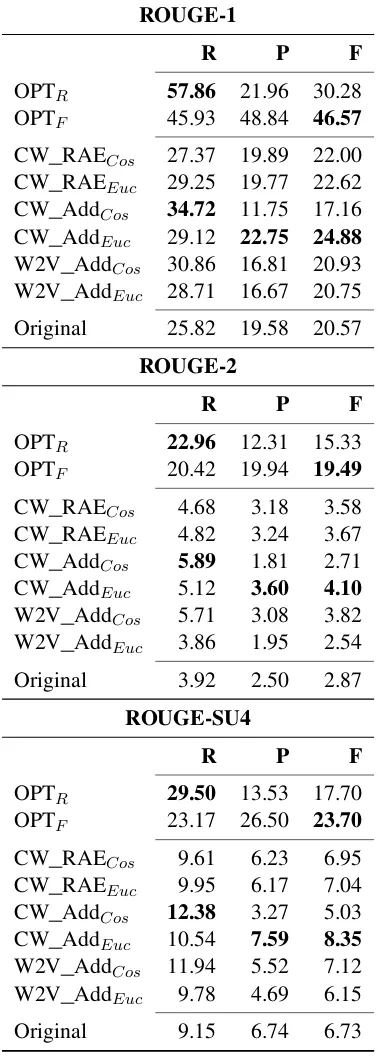
The results from the ROUGE evaluation are com-piled in Table 1. We find for all measures (recall, precision, and F-score), that the phrase embed-dings outperform the original Lin-Bilmes. For re-call, we find that CW_AddCos achieves the high-est result, while for precision and F-score the CW_AddEucperform best. These results are con-sistent for all versions of ROUGE scores reported (1, 2 and SU4), providing a strong indication for phrase embeddings in the context of automatic summarization.
Unfolding RAE on CW vectors and vector ad-dition on W2V vectors gave comparable results w.r.t. each other, generally performing better than original Linn-Bilmes but not performing as well as vector addition of CW vectors.
The results denoted OPT in Table 1 describe the upper bound score, where each row repre-sents optimal recall and F-score respectively. The best results are achieved for R-1 with a maxi-mum recall of 57.86%. This is a consequence of hand created gold standard summaries used in the evaluation, that is, we cannot achieve full recall or F-score when the sentences in the gold stan-dard summaries are not taken from the underly-ing documents and thus, they can never be fully matched using extractive summarization. R-2 and SU4 have lower maximum recall and F-score, with 22.9% and 29.5% respectively.
6.5 Discussion
The results of this paper show great potential for employing word and phrase embeddings in sum-marization. We believe that by using embeddings we move towards more semantically aware sum-marization systems. In the future, we anticipate
1http://metaoptimize.com/projects/wordreprs/ 2https://code.google.com/p/word2vec/
Table 1: ROUGE scores for summaries using dif-ferent similarity measures. OPT constitutes the optimal ROUGE scores on this dataset.
ROUGE-1
R P F
OPTR 57.86 21.96 30.28 OPTF 45.93 48.84 46.57 CW_RAECos 27.37 19.89 22.00 CW_RAEEuc 29.25 19.77 22.62 CW_AddCos 34.72 11.75 17.16 CW_AddEuc 29.12 22.75 24.88 W2V_AddCos 30.86 16.81 20.93 W2V_AddEuc 28.71 16.67 20.75 Original 25.82 19.58 20.57
ROUGE-2
R P F
OPTR 22.96 12.31 15.33 OPTF 20.42 19.94 19.49 CW_RAECos 4.68 3.18 3.58 CW_RAEEuc 4.82 3.24 3.67 CW_AddCos 5.89 1.81 2.71 CW_AddEuc 5.12 3.60 4.10 W2V_AddCos 5.71 3.08 3.82 W2V_AddEuc 3.86 1.95 2.54 Original 3.92 2.50 2.87
ROUGE-SU4
R P F
OPTR 29.50 13.53 17.70 OPTF 23.17 26.50 23.70 CW_RAECos 9.61 6.23 6.95 CW_RAEEuc 9.95 6.17 7.04 CW_AddCos 12.38 3.27 5.03 CW_AddEuc 10.54 7.59 8.35 W2V_AddCos 11.94 5.52 7.12 W2V_AddEuc 9.78 4.69 6.15 Original 9.15 6.74 6.73
improvements for the field of automatic summa-rization as the quality of the word vectors im-prove and we find enhanced ways of composing and comparing the vectors.
It is interesting to compare the results of dif-ferent composition techniques on the CW vec-tors, where vector addition surprisingly
outper-forms the considerably more sophisticated unfold-ing RAE. However, since the unfoldunfold-ing RAE uses syntactic information, this may be a result of using a dataset consisting of low quality text.
In the interest of comparing word embeddings, results using vector addition and cosine similarity were computed based on both CW and Word2Vec vectors. Supported by the achieved results CW vectors seems better suited for sentence similari-ties in this setting.
An issue we encountered with using precom-puted word embeddings was their limited vocab-ulary, in particular missing uncommon (or com-mon incorrect) spellings. This problem is par-ticularly pronounced on the evaluated Opinosis dataset, since the text is of low quality. Future work is to train word embeddings on a dataset used for summarization to better capture the specific se-mantics and vocabulary.
The optimal R-1 scores are higher than R-2 and SU4 (see Table 1) most likely because the score ig-nores word order and considers each sentence as a set of words. We come closest to the optimal score for R-1, where we achieve60% of maximal recall and49% of F-score. Future work is to investigate why we achieve a much lower recall and F-score for the other ROUGE scores.
Our results suggest that the phrase embeddings capture the kind of information that is needed for the summarization task. The embeddings are the underpinnings of the decisions on which sentences that are representative of the whole input text, and which sentences that would be redundant when combined in a summary. However, the fact that we at most achieve 60% of maximal recall sug-gests that the phrase embeddings are not complete w.r.t summarization and might benefit from being combined with other similarity measures that can capture complementary information, for example using multiple kernel learning.
7 Related Work
To the best of our knowledge, continuous vector space models have not previously been used in summarization tasks. Therefore, we split this sec-tion in two, handling summarizasec-tion and continu-ous vector space models separately.
7.1 Continuous Vector Space Models
They employ a FFNN, using a window of words as input, and train the model to predict the next word. This is computed using a big softmax layer that calculate the probabilities for each word in the vocabulary. This type of exhaustive estimation is necessary in some NLP applications, but makes the model heavy to train.
If the sole purpose of the model is to derive word embeddings this can be exploited by using a much lighter output layer. This was suggested by Collobert and Weston (2008), which swapped the heavy softmax against a hinge loss function. The model works by scoring a set of consecutive words, distorting one of the words, scoring the dis-torted set, and finally training the network to give the correct set a higher score.
Taking the lighter concept even further, Mikolov et al. (2013a) introduced a model called Continuous Skip-gram. This model is trained to predict the context surrounding a given word using a shallow neural network. The model is less aware of the order of words, than the previously mentioned models, but can be trained efficiently on considerably larger datasets.
An early attempt at merging word repretations into represenrepretations for phrases and sen-tences is introduced by Socher et al. (2010). The authors present a recursive neural network archi-tecture (RvNN) that is able to jointly learn parsing and phrase/sentence representation. Though not able to achieve state-of-the-art results, the method provides an interesting path forward. The model uses one neural network to derive all merged rep-resentations, applied recursively in a binary parse tree. This makes the model fast and easy to train but requires labeled data for training.
7.2 Summarization Techniques
Radev et al. (2004) pioneered the use of cluster centroids in their work with the idea to group, in the same cluster, those sentences which are highly similar to each other, thus generating a number of clusters. To measure the similarity between a pair of sentences, the authors use the cosine simi-larity measure where sentences are represented as weighted vectors oftf-idf terms. Once sentences are clustered, sentence selection is performed by selecting a subset of sentences from each cluster.
In TextRank (2004), a document is represented as a graph where each sentence is denoted by a vertex and pairwise similarities between sentences
are represented by edges with a weight corre-sponding to the similarity between the sentences. The Google PageRank ranking algorithm is used to estimate the importance of different sentences and the most important sentences are chosen for inclusion in the summary.
Bonzanini, Martinez, Roelleke (2013) pre-sented an algorithm that starts with the set of all sentences in the summary and then iteratively chooses sentences that are unimportant and re-moves them. The sentence removal algorithm ob-tained good results on the Opinosis dataset, in par-ticular w.r.t F-scores.
We have chosen to compare our work with that of Lin and Bilmes (2011), described in Sec. 2.1. Future work is to make an exhaustive comparison using a larger set similarity measures and summa-rization frameworks.
8 Conclusions
We investigated the effects of using phrase embed-dings for summarization, and showed that these can significantly improve the performance of the state-of-the-art summarization method introduced by Lin and Bilmes in (2011). Two implementa-tions of word vectors and two different approaches for composition where evaluated. All investi-gated combinations improved the original Lin-Bilmes approach (using tf-idf representations of sentences) for at least two ROUGE scores, and top results where found using vector addition on CW vectors.
In order to further investigate the applicability of continuous vector representations for summa-rization, in future work we plan to try other sum-marization methods. In particular we will use a method based on multiple kernel learning were phrase embeddings can be combined with other similarity measures. Furthermore, we aim to use a novel method for sentence representation similar to the RAE using multiplicative connections con-trolled by the local context in the sentence.
Acknowledgments
References
Yoshua Bengio, R´ejean Ducharme, Pascal Vincent, and Christian Jauvin. 2003. A neural probabilistic lan-guage model. Journal of Machine Learning Re-search, 3:1137–1155.
Yoshua Bengio. 2002. New distributed prob-abilistic language models. Technical Report 1215, D´epartement d’informatique et recherche op´erationnelle, Universit´e de Montr´eal.
Yoshua Bengio. 2009. Learning deep architectures for ai. Foundations and trendsR in Machine Learning,
2(1):1–127.
Marco Bonzanini, Miguel Martinez-Alvarez, and Thomas Roelleke. 2013. Extractive summarisa-tion via sentence removal: Condensing relevant sen-tences into a short summary. InProceedings of the 36th International ACM SIGIR Conference on Re-search and Development in Information Retrieval, SIGIR ’13, pages 893–896. ACM.
Ronan Collobert and Jason Weston. 2008. A unified architecture for natural language processing: Deep neural networks with multitask learning. In Pro-ceedings of the 25th international conference on Machine learning, pages 160–167. ACM.
Kavita Ganesan, ChengXiang Zhai, and Jiawei Han. 2010. Opinosis: a graph-based approach to abstrac-tive summarization of highly redundant opinions. In
Proceedings of the 23rd International Conference on Computational Linguistics, pages 340–348. ACL. Christoph Goller and Andreas Kuchler. 1996.
Learn-ing task-dependent distributed representations by backpropagation through structure. InIEEE Inter-national Conference on Neural Networks, volume 1, pages 347–352. IEEE.
Alex Graves, Abdel-rahman Mohamed, and Geof-frey Hinton. 2013. Speech recognition with deep recurrent neural networks. arXiv preprint arXiv:1303.5778.
S.S. Haykin. 2009. Neural Networks and Learning Machines. Number v. 10 in Neural networks and learning machines. Prentice Hall.
Geoffrey E Hinton and Ruslan R Salakhutdinov. 2006. Reducing the dimensionality of data with neural net-works. Science, 313(5786):504–507.
Geoffrey E Hinton, Simon Osindero, and Yee-Whye Teh. 2006. A fast learning algorithm for deep be-lief nets. Neural computation, 18(7):1527–1554. Dan Klein and Christopher D Manning. 2003. Fast
ex-act inference with a fex-actored model for natural lan-guage parsing. Advances in neural information pro-cessing systems, pages 3–10.
Alex Krizhevsky, Ilya Sutskever, and Geoff Hinton. 2012. Imagenet classification with deep convolu-tional neural networks. InAdvances in Neural Infor-mation Processing Systems 25, pages 1106–1114.
Hui Lin and Jeff Bilmes. 2011. A class of submodu-lar functions for document summarization. In Pro-ceedings of the 49th Annual Meeting of the Associ-ation for ComputAssoci-ational Linguistics: Human Lan-guage Technologies, pages 510–520. ACL.
Chin-Yew Lin. 2004. Rouge: A package for automatic evaluation of summaries. In Text Summarization Branches Out: Proceedings of the ACL-04 Work-shop, pages 74–81.
Rada Mihalcea and Paul Tarau. 2004. TextRank: Bringing order into texts. In Proceedings of EMNLP, volume 4. Barcelona, Spain.
Tomas Mikolov, Martin Karafi´at, Lukas Burget, Jan Cernock`y, and Sanjeev Khudanpur. 2010. Recur-rent neural network based language model. In IN-TERSPEECH, pages 1045–1048.
Tomas Mikolov, Kai Chen, Greg Corrado, and Jef-frey Dean. 2013a. Efficient estimation of word representations in vector space. ArXiv preprint arXiv:1301.3781.
Tomas Mikolov, Ilya Sutskever, Kai Chen, Greg S Cor-rado, and Jeff Dean. 2013b. Distributed representa-tions of words and phrases and their compositional-ity. InAdvances in Neural Information Processing Systems, pages 3111–3119.
Frederic Morin and Yoshua Bengio. 2005. Hierarchi-cal probabilistic neural network language model. In
AISTATS’05, pages 246–252.
Dragomir R Radev, Hongyan Jing, Małgorzata Sty´s, and Daniel Tam. 2004. Centroid-based summariza-tion of multiple documents. Information Processing & Management, 40(6):919–938.
David E Rumelhart, Geoffrey E Hinton, and Ronald J Williams. 1986. Learning representations by back-propagating errors.Nature, 323(6088):533–536. Gerard Salton and Michael J. McGill. 1986.
Intro-duction to Modern Information Retrieval. McGraw-Hill, Inc., New York, NY, USA.
Richard Socher, Christopher D Manning, and An-drew Y Ng. 2010. Learning continuous phrase representations and syntactic parsing with recursive neural networks. InProceedings of the NIPS-2010 Deep Learning and Unsupervised Feature Learning Workshop.
Richard Socher, Eric H. Huang, Jeffrey Pennington, Andrew Y. Ng, and Christopher D. Manning. 2011. Dynamic Pooling and Unfolding Recursive Autoen-coders for Paraphrase Detection. In Advances in Neural Information Processing Systems 24.
![Figure 6: The structure of an unfolding RAE, ona three word phrase (tations, whiletrix[ x 1 , x 2 , x 3 ] )](https://thumb-us.123doks.com/thumbv2/123dok_us/1503730.691329/5.595.90.288.63.202/figure-structure-unfolding-rae-word-phrase-tations-whiletrix.webp)