Munich Personal RePEc Archive
Split or straight? Some evidence on the
effect of the work shift on Spanish
workers’ well-being and time use
González Chapela, Jorge
Centro Universitario de la Defensa de Zaragoza
14 July 2014
Online at
https://mpra.ub.uni-muenchen.de/57301/
1
SPLIT OR STRAIGHT? SOME EVIDENCE ON THE EFFECT OF THE WORK
SHIFT ON SPANISH WORKERS’ WELL-BEING AND TIME USE
Jorge González Chapela
Centro Universitario de la Defensa de Zaragoza
Address: Academia General Militar, Ctra. de Huesca s/n, 50090 Zaragoza, Spain
Email: [email protected] – Tel: +34 976739834
Abstract
The split work shift has been argued as one of the reasons behind the different Spanish time
schedule, characterized by reduced sleep and a more difficult work-family balance. This paper presents direct evidence on the effect that being on a split shift has on Spanish workers’ well-being and time use. The split shift is found associated to more time spent working in the
market, sleeping, and eating, and less time spent doing housework, caring for children, and at leisure. An increased feeling of being overwhelmed by tasks and having little time to do them
is also found among female split-shifters.
JEL codes: J22, I32.
2 1. INTRODUCTION
One prominent feature of the Spanish labor market is that a significant share of workers are
on a (daytime) split shift, consisting typically of 5 hours of work in the morning, a 2 hour
break in the middle of the day, and another 3 hours of work in the afternoon/evening.1 As a
result, and in comparison with most other European countries, the distribution of the timing
of work in Spain is more spread and presents a sharper dip in the middle of the day (e.g.,
see Amuedo-Dorantes and de la Rica, 2009). It has been argued that the split shift is one of
the main causes of the different Spanish time schedule (e.g., see ARHOE, 2013),
characterized, among other things, by reduced sleep and a more difficult work-family
balance. The purpose of this paper is to present some direct evidence on the effect that
being on a split shift has on Spanish workers’ well-being and time use, conducting separate
analyses for men and women to allow for gender-specific results. The data and methods
used are described in Section 2, the results are presented in Section 3, and the main
conclusions are given in Section 4.
2. DATA AND METHODS
The data for this study come from the Spanish Time Use Survey (STUS) 2002-2003, a
full-scale survey collecting time-use information by the time diary method. Specifically, every
surveyed person aged 10 years or older was asked to list her main activity in each
10-minute interval of the previous 24 hours anchored by 6:00 AM, which is known as the diary
day. The activities reported were then classified into standardized Eurostat activity codes
1
According to the Spanish Survey of Working Conditions, 52.2 percent of workers were on
a split shift in 2003, and 40.2 percent in 2011. By contrast, the share of workers on a
3
(listed in Annex VI of Eurostat, 2004) by the survey agency.2 Also asked for in the STUS is
an important range of labor market and socio-demographic measures, including the
information needed to construct an indicator of role overload (RO). This is a
self-determined measure of well-being defined as having too much to do and not enough time to
do it (Williams, 2008). Worrying about not spending enough time with family is considered
an indicator of role overload, but this specific information was not collected by the STUS.3
The study sample is made up of full-time wage earners aged 18-64 who did not
work between 10:00 PM and 6:00 AM in any of the days included in the weekly work
schedule of the STUS (namely the diary day and the previous six days). I discarded the
self-employed because a priori they seem more likely than wage earners to be able to
self-select into the preferred type of shift, which raises endogeneity concerns. To be considered
as working full time, a worker must spend at least 30 hours per week in the main job. The
information on usual weekly hours worked is obtained from a direct question for those
answering Yes to Do you have the number of weekly hours of work set? For those
answering No, it is obtained from the weekly work schedule, provided that that week is
2
To avoid seasonal distortion in the use of time, the survey was conducted over the course
of one year, distributing the whole survey size evenly between October 2002 and
September 2003. The mean number of activity episodes per diary (21.5), the very low
prevalence of diaries with fewer than seven activity episodes (0.1 percent), and the low
presence of diaries missing two or more basic activities (0.5 percent) indicate diary data of
good quality (Juster, 1985; Robinson, 1985; Fisher et al. 2012).
3
The more recent STUS 2009-2010 did not collect the information needed to construct the
4
reported to be usual. The limitation to daytime workers is intended to reduce heterogeneity.
I also discarded individuals reporting fewer than seven activity episodes on the diary day,
missing two or more of the four basic activities defined in Fisher et al. (2012), or presenting
missing or inconsistent data in some variable used in the study. All this leaves us with
11,159 individuals (and as many other time diaries), of whom 4,289 are women. However,
and in order to isolate more precisely the effects on the allocation of time of being on a split
shift, for the primary time-use analyses the sample is further restricted to individuals whose
diary day is reported to be a regular working day. Thus, diaries pertaining to public
holidays, vacations, or days missed through own illness or other reason, are excluded. Yet,
diaries pertaining to weekend days are included if the diarist reports she worked regularly
on that day. This yields a sample size of 6,800 individuals, of whom 2,596 are women. As
the date of the diary day was randomly assigned by the survey agency, demographic
differences between both samples tend to be small.
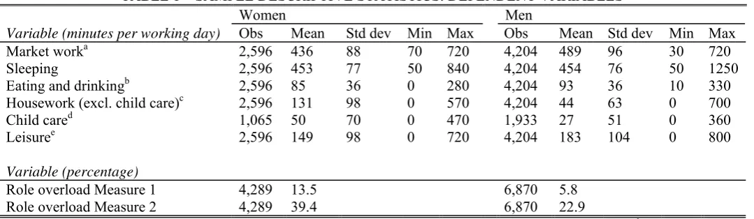
Table 1 presents sample descriptive statistics on the dependent variables by gender.
I use two questions from the individual questionnaire, How often do you feel overwhelmed
by tasks: Very often, Sometimes, orAlmost never? and Do you have little time to do what
you have to do?, to construct two measures of RO. I explore two different measures
because the empirical definition of RO, which is somewhat subjective, influences the
results. Respondents who answer, respectively, Very often and Yes, are considered to suffer
from RO according to our first measure (referred hereafter as ROM1). In our second
measure (ROM2), the RO condition is assigned to those who answer Very often/Sometimes
and Yes. Irrespective of the measure used, women are significantly more likely than men to
5
according to ROM2). A probit model will be used to examine the relationship between RO
and shift type controlling for several other job characteristics and demographics.
The five time activities analyzed here (sleep, eating and drinking, housework, child
care, and leisure) appear often in discussions about work schedules in Spain (e.g., see
ARHOE, 2013). Their definitions, given in Table 1, are standard. As to the proportion of
regular working days presenting zero minutes in some of these activities, it is negligible in
the case of sleep and eating and drinking, very small in the case of leisure, and much larger
in the case of housework (9.6 percent of women and 40.6 percent of men) and, especially,
child care (43.2 percent of mothers and 61.4 percent of fathers). Presumably, zeros pertain
to two kind of individuals: those who never do the activity in question (non-doers), and
doers who, on the diary day, spent no time on it (called reference-period-mismatch zeros by
Stewart, 2013). The latter type introduces measurement error on the dependent variable,
what renders inconsistent the conventional Tobit estimator (Stapleton and Young, 1984).
While the ordinary least squares (OLS) estimator is also inconsistent in the context of the
standard Tobit model, Stoker (1986) has found that if the explanatory variables are
multivariate normally distributed, OLS consistently estimates Tobit’s marginal effects. A
similar conclusion was reached by Greene (1981), whose Monte Carlo study further
suggests that that result is surprisingly robust in the presence of uniformly distributed and
binary variables, but is consistently distorted by the presence of skewed variables such as
chi-squared. Recently, Stewart (2013) has simulated the behavior of the OLS estimator with
time-diary data. In line with Greene (1981) and Stoker (1986), he finds that in the presence
of both doers and non-doers, the OLS beta coefficients are downward biased, but after
6
the true parameter values.4 Therefore, the existing literature suggests that the combination
of a linear specification with a simple OLS estimator may be a reasonable compromise for
specifying and estimating a time-use regression in the presence of observations with zeros.
The reason behind this apparent robustness of OLS may be that the presence of (random)
measurement error on the dependent variable is inconsequential when the estimating model
is linear in parameters.
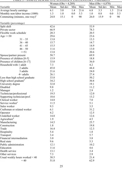
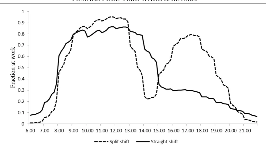
Table 2 presents sample descriptive statistics on the explanatory variables by
gender. The binary variable with the type of shift (split or straight) is constructed from the
question What kind of work shift do you have: Straight or split? 49.6 percent of sample
workers report being on a split shift. (The corresponding population percentage is 51.3.) As
can be seen in Figure 1, which depicts the fraction of sample members who are at work at
each hour of a regular working day, the straight shift takes place primarily in the morning.
The other regressors included in the probit model for RO follow those in Williams (2008),
with the exception of measures of job satisfaction, level of stress, and seeing oneself a
workaholic, which are not available in the STUS. On the other hand, I have included a
sector of employment dummy for reasons given in the next paragraph. The set of
explanatory variables in the time-use regressions does not differ much: I have added
controls for season of the year and day of week, and replaced the measure of usual weekly
hours worked with a measure of minutes worked on the diary day. Moreover, in a couple of
4
The regressors in Stewart’s data-generating process are a dummy and two uniformly
7
instances I have excluded education for reasons given when discussing the results.5 All the
explanatory variables included in the time-use regressions adopt the shapes recommended
by Greene (1981) and Stoker (1986).
Before proceeding with the results, an issue requires some discussion. A worker’s
type of shift might not be completely the result of “random assignment”. For example, an
individual with a strong preference for having free time in the afternoon could select herself
into a sector of employment, occupation, or even company with widespread (morning)
straight-shift jobs. Without controlling for the circumstances underlying the “assignment”
of shift type, the estimated coefficient on the split-shift dummy could be biased.6
Fortunately, we do have information available on the worker’s sector of employment as
well as on her industry and occupation, so that we can hold these characteristics fixed in the
5
This exclusion restriction, coupled with a system homoskedasticity assumption, would
make the feasible generalized least squares (FGLS) estimator to be generally more efficient
than system ordinary least squares (SOLS). However, the efficiency of FGLS comes at the
price of assuming that the regressors of a time-use equation are uncorrelated with the error
terms of all the equations (e.g., see Wooldridge, 2010, Ch.7). SOLS is more robust because
its consistency hinges on the regressors of an equation to be uncorrelated with the error
term of that same equation only. In the absence of cross-equation restrictions on the beta
parameters, SOLS is equivalent to OLS performed equation by equation, which is the
estimation method eventually used.
6
The bias would be in the negative direction if a strong preference for having free time in
the afternoon made the individual more sensitive to feeling role overloaded. The same
8
analyses. Yet, we do not know the degree to which the worker’s company allowed her to
choose shift type. (For example, in Spain the prevalence of split-shift jobs is larger in
smaller companies; INSHT, 2011). Amuedo-Dorantes and de la Rica (2009) have used the
partner’s type of shift to instrument the employee’s type of shift in a model for wages, as
there is evidence that couples time their market work to provide themselves the opportunity
to be together when they are not working (Hamermesh, 2002). However, and continuing
with our example, if this were so, both partners would probably have a preference to be
together in the afternoon, what would invalidate the proposed instrument to be used in our
context. Ideally, the preferred data to this investigation would be generated in a controlled
environment, with an experimenter randomly assigning the type of shift to a set of workers
of known characteristics, then comparing RO and time use outcomes across experimental
groups. These data are still to be generated.
3. RESULTS
3.1 Role overload
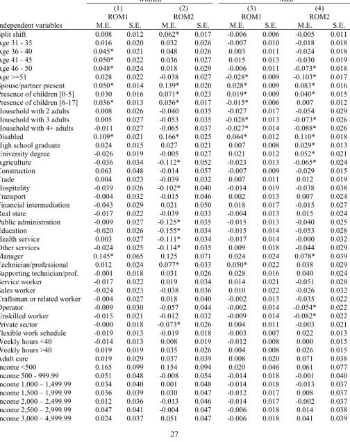
For the RO condition, Table 3 presents probit marginal effects plus associated standard
errors calculated with the delta method. All marginal effects are obtained as
x xj 1
x xj 0
, where is the standard normal cdf, and are estimated by
plugging in the probit estimate ˆ and then averaging across observations. The first two
columns present the results for women, whereas men’s results are in Columns (3) and (4).
Results for ROM1 (our narrower definition of RO) are in odd columns, while those for
ROM2 appear in even columns.
The type of shift is not associated with the incidence of RO according to ROM1:
9
and statistically not different from zero at 0.05 level. Factors associated with ROM1 for
both women and men are age, presence of a spouse/partner in the household, presence of
children aged 6-17, and disability status. For women, the likelihood of suffering from RO
increases with age up until the 41-45 age interval, decreasing from that moment on. In the
case of men, the only statistically significant result is that a male aged 51+ is 0.028 less
likely to suffer from RO than a comparable male aged 30 or younger. On average, women
are 0.050 more likely to experience RO when a spouse/partner is present in the household,
whereas the corresponding effect for men is 0.028. Since the average incidence of ROM1
is, respectively, 0.135 and 0.058, the presence of a spouse/partner increases that probability
by around 37 percent for women and 48 percent for men. The presence of children aged
6-17 increases the probability of feeling role overloaded by 0.036 in the case of women, but
decreases that probability by 0.015 in the case of men. Having a physical or mental
disability has a strong influence on experiencing RO, whose incidence increases on average
by approximately 81 percent in the case of women and 110 percent in the case of men. The
only factor associated with ROM1 for women but not for men is having a managerial job,
which, on average, increases the likelihood of suffering from RO by around 107 percent.
(This managerial job effect is with respect to a comparable female clerical worker.) Factors
associated with ROM1 for men but not for women are the presence of children of
pre-school age,7 the presence of other adults, and having a technical/professional job, which
change the incidence of RO by approximately +33, -47, and +86 percent, respectively.
7
The effect associated to the presence of children of pre-school age is indeed larger for
10
Considering the broader definition of RO (ROM2) has a pronounced effect on the
impact of being on a split shift for women, whose estimated marginal effect becomes much
larger and statistically different from zero. Holding other factors fixed, female full-time
wage earners are on average 0.062 more likely to experience RO when being on a split
shift, which represents a 16 percent increase in the average incidence of ROM2 (0.394). On
the other hand, the estimated marginal effect of having a managerial job is now somewhat
smaller and statistically not different from zero. By contrast, the type of shift is again
unrelated to the incidence of RO for men, but having a managerial job becomes significant:
On average, the incidence of ROM2 is 34 percent larger for a male manager than for a
comparable male clerical worker. Jobs in the agriculture, hospitality, public administration,
education, health, and personal services industries now offer some protection to women
with respect to RO. In the case of men, it is working in the agriculture what is now
associated to a lower likelihood of RO.
The sector of employment is unrelated to suffering from RO except in the case of
women when using ROM2. In that instance, female full-time wage earners working in the
private sector are 0.073 less likely to experience RO than comparable women working in
the public sector. A Wald test for the joint exclusion of the usual weekly hours of work
dummies does not reject the null of no significance in all instances, and the same occurs
with the dummies for household income. The estimated marginal effect associated to
having a flexible work schedule presents the expected negative sign in three out of the four
estimations, but it is small and does not attain statistical significance.
The journey to work, which exposes us to environmental and psychological
stressors such as noise, crowds, and time pressure, is generally considered a daily hassle.
11
duration or daily frequency could have a bearing on the incidence of RO.8 A potential
problem is that these characteristics can be, to some extent, chosen by the worker in order
to deal with RO. If the circumstances underlying those choices were unknown or
unobserved to the econometrician, commuting would be endogenous, whereby establishing
the relationship between commuting and RO (or other measure of well-being) would
require a more elaborate analysis than that conducted here. I have just re-estimated the
model for RO on sample members whose diary day was reported to be a regular working
day, adding either the duration of the (one-way) commute or the number of commuting
episodes on that day to the set of explanatory variables.9 Moreover, and in an attempt to
reduce endogeneity concerns, the model including the former regressor was run on home
owners only, as these may be less inclined than tenants to move and thus to adjusting their
commute duration by changing residential location. (This selection criterion reduced the
sample an additional 14 percent.) The estimated coefficient associated to the commute
duration is positive and relatively large, being statistically different from zero at or around
0.05 level in three out of the four cases considered. For women, residing at 10 minutes
more from the job increases the likelihood of suffering from RO by around 10 percent in
the case of ROM1 and 4 percent in the case of ROM2. For men the corresponding increases
are 7 and 4 percent. Therefore, the commute duration has a larger bearing on those who feel
8
Koslowsky et al. (1995) survey the physical and psychological consequences of
commuting, and discuss coping techniques.
9
The average duration of the commute is not much different for split-shift and straight-shift
workers (24.8 vs. 26.3 minutes, respectively), but the mean number of daily commuting
12
overwhelmed by tasks very often than on those who feel overwhelmed just sometimes. As
to the number of daily commuting episodes, its estimated coefficient is generally positive
but small, not attaining statistical significance in any estimation. Neither the different
samples nor the inclusion of commuting characteristics alter the main findings regarding
the type of shift.
3.2 Time allocation
Discussions about the possible impact on the allocation of time of the straight shift
implicitly assume that time worked is the same for straight- and split-shifters. As a matter
of fact, this is not so. A tabulation of working time in the main job by type of shift reveals
that sample full-time wage earners being on a split shift work, on average, 60 minutes more
each regular working day than straight-shifters, i.e. 5.0 hours more per week if working 5
days a week. This difference, obtained from time diary estimates, excludes coffee and other
breaks as well as on-the-job training. The gap derived from the weekly work schedule
measure, which includes paid breaks, training, and time in secondary jobs, is similar: 4.9
hours more per week. Even among workers having the number of weekly hours of work set
there is a gap, in this case of 1.5 hours more per week. The same pattern is observed by
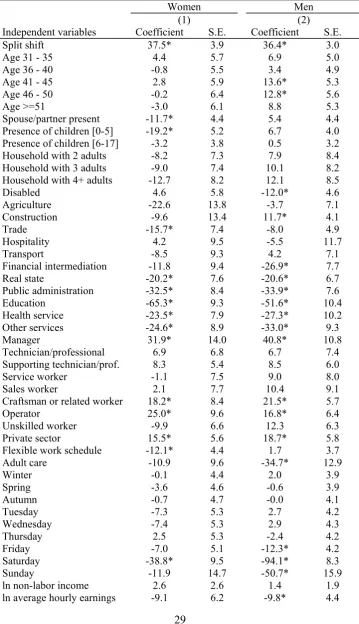
gender. In an attempt to better isolate the impact of being on a split shift on time worked, a
linear regression for minutes spent working on regular working days was estimated
separately for women and men.10 Results are presented in Table 4. After the effects of the
10
With respect to the baseline specification for the allocation of time, I have excluded
education plus replaced household income (which is endogenous in a model for working
time) with measures of the hourly wage rate and non-labor income. The hours of work
13
other regressors are netted out, full-time wage earners having a split shift still spend some
37 minutes more on the job than straight-shifters. This is the reason why time spent on the
job is included among the explanatory variables for the allocation of time equations. By
contrast, commuting time is not included, for this time saved by being on a straight shift
(implicit in the figures given in note 9) could be devoted to alternative, less committed
activities.
Tables 5 and 6 present OLS estimates for the allocation of time separately for
women and men. In both tables, the estimations in columns (1), (2), (3), and (5), pertaining,
respectively, to time spent sleeping, eating and drinking, doing housework, and at leisure,
are obtained on all individuals whose diary day is reported to be a regular working day.
However, the estimation for child care (column (4)) is obtained on the subsample of parents
only, which relaxes the assumption that child care time falls continuously to zero in
response to variations in the explanatory variables. Since the latter group might not be a
random sample from the former, a standard sample selection correction was implemented.
First, I estimated a probit model for the decision to have children over the entire sample of
individuals whose diary day is a regular working day, relating the probability of having
reduces concerns about division bias (Borjas, 1980). Of course, other sort of biases might
be affecting the hours-wage relationship, as the negative wage coefficients presented in
Table 4 seem to suggest. Instrumenting the wage rate with the worker’s educational
attainment makes its estimated coefficient to be positive (although not statistically different
from zero) in the male subsample, leaving almost unchanged the estimated coefficient on
the split shift dummy. This result is in line with the lack of association between wages and
14
children to the whole set of time-use regressors. Then, I obtained the estimated inverse
Mills ratio for each individual, which was included in the OLS regression for child care run
on parents only. Given the frequently observed negative correlation between parents’
education and completed fertility (e.g., see Michael, 1973), the second-stage OLS
regression excludes education from the explanatory variables, which was thus used to
further identify the parameters of the sample selection model. The evidence presented in
Gimenez-Nadal and Molina (2013) suggests that this exclusion restriction suits particularly
men’s behavior. The standard errors in Tables 5 and 6 are robust to hereroskedasticity, but
those in column (4) are additionally corrected for the presence of generated regressors
using the procedure in Arellano and Meghir (1992, Appendix B.4).
Having a split shift is associated with more time spent sleeping: 14 minutes more
per regular working day in the case of women and 10 minutes more in the case of men.
Estimates are precise and attain statistical significance. Thus, for concreteness, an average
female wage earner working full time on a split shift is predicted to sleep 463 minutes (7.7
hours) on a regular working day, but if that woman went to a straight shift her time spent
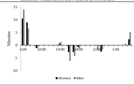
sleeping would fall to 449 minutes (7.5 hours). To investigate the immediate reason behind
this difference, I have re-estimated the regression for minutes of sleep on observations for
each hour of the day (i.e., time spent sleeping between 6 AM and 7 AM, between 7 AM and
8 AM, and so on and so forth). Figure 2 depicts the sign and size of the statistically
significant effects associated to having a split shift, by time of day and sex. On average,
workers having a straight shift wake up earlier in the morning than comparable
split-shifters, but are not asleep generally at earlier times at night. Although straight-shifters take
a (longer) nap after returning home in the late afternoon, its duration does not compensate
15
schedules affect the timing of market work and sleep: Americans residing in the central and
mountain time zones of the US (where television shows from late afternoon onward appear
1 nominal hour earlier than in the eastern and pacific zones), are less likely to be watching
television between 11:00 PM and 11:15 PM, and more likely to be working between 8:00
AM and 8:15 AM, than comparable Americans living in other parts of the country. This
result suggests that advancing the time of television shows in Spain could make
straight-shifters to sleep more (although it would not reduce the sleeping gap with split-straight-shifters if
these responded in the same manner). In any case, the difference in mean sleep times
associated to the type of shift seems of little importance, as studies of accumulated sleep
loss suggest that gradual performance impairment (i.e., reduced attention, cognitive
functioning, and psychomotor performance) starts when sleep duration falls below 7 hours
(Akerstedt et al., 2009).
The split shift is also associated with more time spent eating and drinking on regular
working days: some 7 minutes more for women and 6 minutes more for men. Estimates are
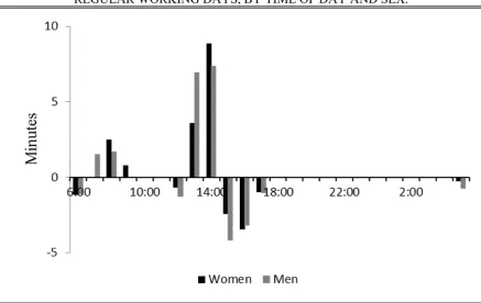
precise and attain statistical significance. Figure 3, which is constructed analogously to
Figure 2, shows that this difference derives essentially from the duration of the lunch. (On
average, split-shifters spend more time having breakfast, but the gap, of about 2 minutes, is
then compensated by straight-shifters taken a (longer) lunch break between 12:00 PM and
1:00 PM.) I have re-estimated the regression for minutes spent eating and drinking but just
for the interval 1:00 PM to 5:00 PM, distinguishing among having the lunch at home, on
the job, or in a restaurant. On average, being on a split shift increases the duration of the
lunch at home by about 6 minutes in the case of women and 3 minutes in the case of men.
Its effect on lunches in restaurants is also positive but smaller (just 1 minute more, although
16
unrelated to the duration of the lunch. The split shift is also associated with an increase in
the proportions of female full-time wage earners who have the meal at home and in a
restaurant,11 which, given the longer duration of the lunch in those places, seems to partly
account for its effect on time spent eating and drinking. For male counterparts the
conclusion is less clear cut, as being on a split shift is associated with an increase in the
proportion of those having lunch in a restaurant, but also with a significant decrease in the
share of those who eat at home.
The other three activities are negatively associated with having a split shift. Female
full-time wage earners being on a split shift spend approximately 11 minutes less on
domestic activities on a regular working day than comparable straight-shifters. Male
counterparts spend about 10 minutes less. Although not shown in the tables, the main
contributor to these reductions is time spent shopping for consumer goods and services,12
which shrinks 4.5 minutes for women and 3.5 minutes for men. All these effects are
precisely measured and achieve statistical significance. The lower quantity of time spent
shopping on regular working days could be made up by shopping more intensively on days
11
Among full-time wage earners who consider the diary day to be a regular working day,
the percentages of split-shift (respectively, straight-shift) women who have the meal at
home, on the job, and in a restaurant between 1:00 PM and 5:00 PM are 78.0 (75.2), 10.0
(10.5), and 6.2 (2.5), respectively. (Estimates do not add up to 100 because some workers
report other places for having the lunch.) For men, the corresponding percentages are 64.0
(72.0), 14.2 (10.5), and 7.4 (4.9).
12
Included here are errands presuming visits to shops, offices, institutions, etc., such as
17
off. To investigate this possibility, I have estimated regressions for shopping time on the
full sample of diaries, including among the regressors a binary variable equal to one for
days off and an interaction term between this and the dummy for being on a split shift. This
interaction allows the effect of being on a split shift to depend on the type of day. For
female full-time wage earners on a split shift, the estimated reduction in shopping time on
regular working days is again 4.5 minutes (S.E. = 1.7), whereas the estimate on the
interaction term is 4.1, S.E. = 3.4. Adding up both estimates we conclude that female
split-shifters do not spend more time shopping on days off than comparable straight-split-shifters. For
male counterparts the conclusion is the same, because the corresponding estimates are -3.1,
S.E. = 0.9, and 1.9, S.E. = 2.0. There is evidence that by shopping more intensively,
households lower the price paid for a given basket of goods (e.g., see Aguiar and Hurst,
2007). But the presumed higher price paid by split-shifters does not necessarily imply a
reduction in their welfare, as the shopping time saved could be devoted to other, preferable
activities (sleep, eating and drinking, etc.; notice that time worked in the market is being
kept constant.)
Mothers being on a split shift spend 5 minutes less per regular working day on child
care activities than comparable mothers having a straight shift, but the effect is not
precisely measured and does not attain statistical significance. For fathers, being on a split
shift is also associated to a reduction in child care time, this time of approximately 9
minutes and measured precisely. Thus, for concreteness, an average full-time wage earner
father being on a straight shift is predicted to devote some 42 minutes to child care on a
regular working day, but if that father went to a split shift his corresponding child care time
would fall to 33 minutes. I followed the procedure described in the previous paragraph to
18
sample, the estimated reduction in child care by mothers on a split shift is approximately 7
minutes (S.E. = 4.5) per regular working day, whereas the estimate on the interaction
between having a split shift and being a day off is essentially zero. For fathers, the
corresponding estimates are -9.5, S.E. = 2.8, and 13.7, S.E. = 5.2, which indicate that
fathers on a split shift spend 4 minutes more caring for their children on days off than
comparable fathers having a straight shift. Thus, a father working 5 days a week under a
split shift devotes some 39 minutes less to child care over the course of the week than a
comparable father being on a straight shift.
Also affected by the type of shift is the time spent at leisure on regular working
days. Being on a split shift reduces that time by approximately 9 minutes for both women
and men. Both effects attain statistical significance. For women, the main contributor to
that reduction is the domain of social life and entertainment (e.g., visiting and receiving
visitors or watching movies in cinema), which shrinks 4.5 minutes. For men, the reduction
is mainly due to sports and outdoor activities, which, as a group, are 10 minutes smaller
having a split shift. The evidence suggests that, in comparison with males being on a
straight shift, male split-shifters do not devote more time to sports and outdoor activities on
days off to make up for the time lost on regular working days. However, female
split-shifters do devote some 7 minutes more to social life and entertainment on days off than
comparable women having a straight shift: In the full sample, and for a dependent variable
measuring minutes spent on social life and entertainment only, the estimated coefficient on
the split shift dummy is -7.9 (S.E. = 3.3), whereas the estimate on the interaction between
having a split shift and being a day off is 15.2 (S.E. = 7.2). Thus, a female wage earner
19
less on social life and entertainment over the course of the week than a comparable woman
having a straight shift.
The effects on the allocation of time of being on a split shift do not seem much
different across sexes. To test formally the equality of effects for men and women, I have
re-estimated each time-use regression on the combined sample of men and women,
allowing the intercept and all slope coefficients to depend on gender. (If we just allowed the
intercept and the split shift dummy to depend on gender, we would be assuming that the
remaining regressors exert the same effect for men and women. A cursory inspection to
Tables 5 and 6 strongly suggests that this assumption is not correct, and, indeed, it is
soundly rejected by a formal test in all instances except the equation for eating and
drinking.) Then, I have tested whether the interaction term between having a split shift and
the dummy for gender is statistically significant using a robust t-statistic. As some of the
sample men and women are married together, the standard errors are not only robust to
heteroskedasticity, but also to arbitrary within-household correlation. In all five instances,
the claim that the effect on the allocation of time of having a split shift is the same for men
and women is well within confidence bounds. But then, why is being on a split shift a
significant predictor of ROM2 for women only? One possible explanation is that the
common absolute time variations represent different relative time changes by gender. For
example, female straight-shifters spent, on average, 157 minutes at leisure on regular
working days, whereas male counterparts spend 200 minutes. Hence, the common
reduction of about 9 minutes per day brought about by the split shift is relatively more
important for women. However, the marginal effect of being on a split shift suffers little
20
suggesting that the reduction in leisure associated to the split shift is not the reason behind
the increased incidence of ROM2.
4. CONCLUSION
We have found evidence that the type of daytime work shift (split or straight) has a bearing
on the allocation of time on regular working days among Spanish full-time wage earners.
Other things equal, being on a split shift is associated with more time spent working in the
market, sleeping, and eating and drinking, and less time spent doing housework, caring for
children, and at leisure. The lower quantity of leisure is partly made up on days off in the
case of women, but not in the case of men. By contrast, split-shifters’ lower quantity of
time spent caring for children is partly made up on days off by fathers, but not by mothers.
Split-shifters’ lower quantity of domestic work on regular working days derives mainly
from a reduction in time spent shopping for consumer goods and services. This reduction is
not compensated by shopping more intensively on days off, which suggests that
split-shifters may be paying more for the same basket of goods than comparable straight-split-shifters.
Straight-shifters do sleep less on regular working days because they wake up earlier in the
morning, are not asleep generally at earlier times at night, and the duration of their nap does
not compensate for the lost sleep in the morning. This finding is in stark contrast to the
prediction that the straight shift will increase night’s rest on regular working days
(ARHOE, 2013, p. 88-89). The sleep loss (between 10-15 minutes) does not seem large
enough so as to impair performance.
Although the effects on the allocation of time associated to the type of shift are
similar across sexes, this is not so for the incidence of role overload. Among male full-time
wage earners the type of shift is unrelated to the role overload condition, but being on a
21
having little time to do them) among female counterparts. However, when the definition of
role overload is narrowed to feeling very often overwhelmed by tasks, the type of shift
appears as irrelevant among women too. The evidence suggests that the reduction in the
quantity of daily leisure associated to the split shift is not the reason behind the higher
incidence of role overload broadly considered among female split-shifters.
REFERENCES
Aguiar, Mark, and Erik Hurst. 2007. Life-cycle prices and production. American
Economics Review 97(5):1533-1559.
Akerstedt, Torbjörn, Peter M. Nilsson, and Göran Kecklund. 2009. Sleep and recovery. In
Current perspectives on job-stress recovery: Research in occupational stress and
well being Volume 7. Eds. S. Sonnentag, P.R. Perrewé, and D.C. Ganster. Emerald
Group Publishing Limited.
Amuedo-Dorantes, Catalina, and Sara de la Rica. 2009. The timing of work and
work-family conflicts in Spain: Who has a split work schedule and why? IZA Discussion
Paper No. 4542.
Arellano, Manuel, and Costas Meghir. 1992. Female labour supply and on-the-job search:
an empirical model estimated using complementary data sets. Review of Economic
Studies 59:537-557.
ARHOE. 2013. Horarios, flexibilidad y productividad. VII Congreso Nacional para
Racionalizar los Horarios Españoles. Asociación para la Racionalización de los
Horarios Españoles.
Borjas, George J. 1980. The relationship between wages and weekly hours of work: The
22
Eurostat. 2004. Guidelines on harmonized European time use surveys. Luxembourg: Office
for Official Publications of the European Communities.
Fisher, Kimberly, Jonathan Gershuny, Evrim Altintas, and Anne H. Gauthier. 2012.
Multinational Time Use Study. User’s Guide and Documentation. Version 5 –
updated. University of Oxford.
Gimenez-Nadal, J. Ignacio, and Jose Alberto Molina. 2013. Parents’ education as a
determinant of educational childcare time. Journal of Population Economics
26:719-749.
Greene, William H. 1981. On the asymptotic bias of the Ordinary Least Squares estimator
of the Tobit model. Econometrica 49(2):505-513.
Hamermesh, Daniel S. 2002. Timing, togetherness and time windfalls. Journal of
Population Economics 15:601-623.
Hamermesh, Daniel S., Caitlin Knowles Myers, Mark L. Pocock. 2008. Cues for timing
and coordination: latitude, Letterman, and longitude. Journal of Labor Economics
26(2):223-246.
INSHT. 2011. VII Encuesta Nacional de Condiciones de Trabajo. Instituto Nacional de
Seguridad e Higiene en el Trabajo.
Juster, F. Thomas. 1985. The validity and quality of time use estimates obtained from recall
diaries. In Time, Goods, and Well-Being, edited by F. Thomas Juster and Frank P.
Stafford, pp.63-92. Institute for Social Research, University of Michigan.
Koslowsky, Meni, Avraham N. Kluger, and Mordechai Reich. 1995. Commuting stress.
Causes, effects, and methods of coping. New York and London: Plenum Press.
Michael, Robert T. 1973. Education and the derived demand for children. Journal of
23
Robinson, John P. 1985. The validity and reliability of diaries versus alternative time use
measures. In Time, Goods, and Well-Being, edited by F. Thomas Juster and Frank P.
Stafford, pp.33-62. Institute for Social Research, University of Michigan.
Stapleton, David C., and Douglas J. Young. 1984. Censored normal regression with
measurement error on the dependent variable. Econometrica 52(3):737-760.
Stewart, Jay. 2013. Tobit or not Tobit? Journal of Economic and Social Measurement
38:263-290.
Stoker, Thomas M. 1986. Consistent estimation of scaled coefficients. Econometrica
54(6):1461-1481.
Williams, Cara. 2008. Work-life balance of shift workers. Perspectives on Labour and
Income 20(3):15-26.
Wooldridge, Jeffrey M. 2010. Econometric Analysis of Cross Section and Panel Data,
24
TABLE 1—SAMPLE DESCRIPTIVE STATISTICS: DEPENDENT VARIABLES
Women Men
Variable (minutes per working day) Obs Mean Std dev Min Max Obs Mean Std dev Min Max
Market worka 2,596 436 88 70 720 4,204 489 96 30 720
Sleeping 2,596 453 77 50 840 4,204 454 76 50 1250
Eating and drinkingb 2,596 85 36 0 280 4,204 93 36 10 330
Housework (excl. child care)c 2,596 131 98 0 570 4,204 44 63 0 700
Child cared 1,065 50 70 0 470 1,933 27 51 0 360
Leisuree 2,596 149 98 0 720 4,204 183 104 0 800
Variable (percentage)
Role overload Measure 1 4,289 13.5 6,870 5.8
Role overload Measure 2 4,289 39.4 6,870 22.9
Notes:a: Excludes coffee and other breaks and on-the-job training, but includes time in secondary jobs. b: Includes lunch
break at work. c: Gathers time spent on food management, household upkeep, making and care for textiles, gardening and
pet care, construction and repairs, shopping for consumer goods and services, household management, and help to adult
family members. d: Parents only. e: Gathers time spent on social life and entertainment, sports and outdoor activities,
25
TABLE 2—SAMPLE DESCRIPTIVE STATISTICS: EXPLANATORY VARIABLES
Women (Obs = 4,289) Men (Obs = 6,870)
Variable Mean Std dev Min Max Mean Std dev Min Max
Average hourly earnings 6.1 3.0 1.4 21.6 6.8 3.3 1.3 21.6
Monthly non-labor income (1000) 1.3 1.0 0.0 5.3 1.0 0.8 0.0 5.3
Commuting (minutes, one-way)a 24.8 15.1 0 90 26.0 15.9 0 90
Variable (percentage)
Split shift 42.6 53.9
Private sector 66.9 78.3
Flexible work schedule 20.3 20.5
Age <=30 29.6 23.6
31 – 35 13.8 13.3
36 – 40 15.7 14.7
41 – 45 15.5 14.9
46 – 50 11.6 13.0
>=51 13.8 20.6
Spouse/partner present 58.7 69.9
Presence of children [0-5] 15.9 18.8
Presence of children [6-17] 33.0 36.0
Household with 1 adult 7.3 4.2
2 adults 45.0 44.4
3 adults 21.6 24.0
4+ adults 26.1 27.4
Less than high school graduate 33.8 50.2
High school graduateb 34.2 30.8
University degree 32.0 19.1
Disabled 9.8 11.2
Manager 1.2 2.9
Technician/professional 19.5 12.0
Supporting technician/prof. 18.6 13.2
Clerical worker 14.8 7.0
Service workerc 11.5 5.1
Sales worker 9.3 3.5
Craftsman or related worker 6.1 31.2
Operator 4.2 12.5
Unskilled worker 14.8 12.6
Agricultured 1.9 4.5
Manufacturing 14.5 25.7
Construction 1.8 19.8
Trade 16.4 12.3
Hospitality 5.4 1.8
Transport 3.4 5.7
Financial intermediation 3.0 3.8
Real state 9.6 5.3
Public administration 12.1 10.2
Education 11.6 4.6
Health service 13.1 3.4
Other services 7.3 2.9
Usual weekly hours worked < 40 38.5 21.4
26
> 40 9.7 15.7
Owner 86.2 84.7
Adult care 3.7 2.1
Household net monthly income < 500 0.8 0.7
500 – 999.99 7.8 10.7
1,000 – 1,499.99 18.2 24.9
1,500 – 1,999.99 21.1 22.2
2,000 – 2,499.99 19.7 16.6
2,500 – 2,999.99 12.5 10.3
3,000 – 4,999.99 17.0 12.6
≥5,000 2.9 2.0
Winter 27.1 26.8
Spring 26.6 26.7
Summer 23.2 23.6
Autumn 23.1 22.9
Monday 12.9 12.6
Tuesday 13.0 13.0
Wednesday 12.5 12.3
Thursday 12.9 12.5
Friday 16.4 16.6
Saturday 16.1 16.1
Sunday 16.2 16.9
Regular working day 62.0 62.4
Notes: Money variables are in euros of 2002/2003. Labor market measures pertain to the main job. a: Regular
working days. b: Includes those with vocational training. c: Includes the military. d: Includes extractive
27
TABLE 3—PROBIT EQUATIONS FOR SUFFERING FROM ROLE OVERLOAD (MARGINAL EFFECTS)
Women Men
(1) (2) (3) (4)
ROM1 ROM2 ROM1 ROM2
Independent variables M.E. S.E. M.E. S.E. M.E. S.E. M.E. S.E.
Split shift 0.008 0.012 0.062* 0.017 -0.006 0.006 -0.005 0.011
Age 31 - 35 0.016 0.020 0.032 0.026 -0.007 0.010 -0.018 0.018
Age 36 - 40 0.045* 0.021 0.048 0.026 0.003 0.011 -0.024 0.018
Age 41 - 45 0.050* 0.022 0.036 0.027 0.015 0.013 -0.030 0.019
Age 46 - 50 0.048* 0.024 0.018 0.029 -0.006 0.011 -0.073* 0.018
Age >=51 0.028 0.022 -0.038 0.027 -0.028* 0.009 -0.103* 0.017
Spouse/partner present 0.050* 0.014 0.139* 0.020 0.028* 0.009 0.083* 0.016
Presence of children [0-5] 0.030 0.016 0.071* 0.023 0.019* 0.009 0.040* 0.015
Presence of children [6-17] 0.036* 0.013 0.056* 0.017 -0.015* 0.006 0.007 0.012
Household with 2 adults 0.008 0.026 -0.040 0.035 -0.027 0.017 -0.054 0.029
Household with 3 adults 0.005 0.027 -0.053 0.035 -0.028* 0.013 -0.073* 0.026
Household with 4+ adults -0.011 0.027 -0.065 0.037 -0.027* 0.014 -0.088* 0.026
Disabled 0.109* 0.021 0.166* 0.025 0.064* 0.012 0.110* 0.018
High school graduate 0.024 0.015 0.027 0.021 0.007 0.008 0.029* 0.013
University degree -0.026 0.019 -0.005 0.027 0.021 0.012 0.052* 0.021
Agriculture -0.036 0.034 -0.112* 0.052 -0.023 0.013 -0.065* 0.024
Construction 0.063 0.048 -0.014 0.057 -0.007 0.009 -0.029 0.015
Trade 0.004 0.023 -0.039 0.032 0.007 0.011 0.012 0.019
Hospitality -0.039 0.026 -0.102* 0.040 -0.014 0.019 -0.038 0.038
Transport -0.004 0.032 -0.015 0.046 0.002 0.013 0.007 0.024
Financial intermediation -0.043 0.029 0.021 0.050 0.018 0.017 -0.015 0.027
Real state -0.017 0.022 -0.039 0.033 -0.004 0.013 0.015 0.024
Public administration -0.009 0.027 -0.125* 0.035 -0.015 0.013 -0.040 0.025
Education -0.020 0.026 -0.155* 0.034 -0.015 0.014 -0.053 0.028
Health service 0.003 0.027 -0.111* 0.034 -0.017 0.014 -0.000 0.032
Other services -0.024 0.025 -0.114* 0.035 0.009 0.018 -0.044 0.029
Manager 0.145* 0.065 0.125 0.071 0.024 0.024 0.078* 0.039
Technician/professional 0.012 0.024 0.077* 0.033 0.050* 0.022 0.038 0.029
Supporting technician/prof. -0.001 0.018 0.031 0.026 0.028 0.016 0.040 0.024
Service worker -0.017 0.022 0.019 0.034 0.014 0.021 -0.051 0.028
Sales worker -0.024 0.023 -0.038 0.036 0.010 0.022 -0.026 0.032
Craftsman or related worker -0.004 0.027 0.018 0.040 -0.002 0.013 -0.035 0.022
Operator -0.009 0.030 -0.057 0.044 -0.002 0.014 -0.054* 0.022
Unskilled worker -0.015 0.021 -0.012 0.032 -0.009 0.014 -0.082* 0.022
Private sector -0.000 0.018 -0.073* 0.026 0.004 0.011 -0.003 0.021
Flexible work schedule -0.019 0.013 -0.019 0.018 -0.003 0.007 0.022 0.013
Weekly hours <40 -0.014 0.013 0.008 0.019 -0.012 0.008 0.000 0.015
Weekly hours >40 0.019 0.019 0.035 0.026 0.004 0.008 0.026 0.015
Adult care 0.019 0.029 0.037 0.039 0.008 0.020 0.071 0.038
Income <500 0.165 0.099 0.154 0.094 0.020 0.046 0.061 0.077
Income 500 - 999.99 0.051 0.048 -0.008 0.054 -0.014 0.018 -0.001 0.040
Income 1,000 – 1,499.99 0.034 0.040 0.001 0.048 -0.014 0.018 -0.013 0.037
Income 1,500 – 1,999.99 0.036 0.039 0.030 0.047 -0.012 0.017 0.008 0.037
Income 2,000 – 2,499.99 0.012 0.036 -0.013 0.046 -0.014 0.017 -0.002 0.037
Income 2,500 – 2,999.99 0.047 0.041 -0.004 0.047 -0.006 0.018 0.014 0.038
28
Log-likelihood -1,615 -2,713 -1,427 -3,490
R-squared 0.050 0.057 0.060 0.057
Observations 4,289 4,289 6,870 6,870
Notes: All estimations include an intercept. Standard errors are calculated with the delta method. R-squared equals one
minus the ratio of the log likelihood of the fitted function to the log likelihood of a function with only an intercept.
Unreported categories: Age <=30, 1-adult household, less than high school graduate, manufacturing, clerical worker,
29
TABLE 4—MINUTES OF WORK ON REGULAR WORKING DAYS. OLS ESTIMATES
Women Men
(1) (2)
Independent variables Coefficient S.E. Coefficient S.E.
Split shift 37.5* 3.9 36.4* 3.0
Age 31 - 35 4.4 5.7 6.9 5.0
Age 36 - 40 -0.8 5.5 3.4 4.9
Age 41 - 45 2.8 5.9 13.6* 5.3
Age 46 - 50 -0.2 6.4 12.8* 5.6
Age >=51 -3.0 6.1 8.8 5.3
Spouse/partner present -11.7* 4.4 5.4 4.4
Presence of children [0-5] -19.2* 5.2 6.7 4.0
Presence of children [6-17] -3.2 3.8 0.5 3.2
Household with 2 adults -8.2 7.3 7.9 8.4
Household with 3 adults -9.0 7.4 10.1 8.2
Household with 4+ adults -12.7 8.2 12.1 8.5
Disabled 4.6 5.8 -12.0* 4.6
Agriculture -22.6 13.8 -3.7 7.1
Construction -9.6 13.4 11.7* 4.1
Trade -15.7* 7.4 -8.0 4.9
Hospitality 4.2 9.5 -5.5 11.7
Transport -8.5 9.3 4.2 7.1
Financial intermediation -11.8 9.4 -26.9* 7.7
Real state -20.2* 7.6 -20.6* 6.7
Public administration -32.5* 8.4 -33.9* 7.6
Education -65.3* 9.3 -51.6* 10.4
Health service -23.5* 7.9 -27.3* 10.2
Other services -24.6* 8.9 -33.0* 9.3
Manager 31.9* 14.0 40.8* 10.8
Technician/professional 6.9 6.8 6.7 7.4
Supporting technician/prof. 8.3 5.4 8.5 6.0
Service worker -1.1 7.5 9.0 8.0
Sales worker 2.1 7.7 10.4 9.1
Craftsman or related worker 18.2* 8.4 21.5* 5.7
Operator 25.0* 9.6 16.8* 6.4
Unskilled worker -9.9 6.6 12.3 6.3
Private sector 15.5* 5.6 18.7* 5.8
Flexible work schedule -12.1* 4.4 1.7 3.7
Adult care -10.9 9.6 -34.7* 12.9
Winter -0.1 4.4 2.0 3.9
Spring -3.6 4.6 -0.6 3.9
Autumn -0.7 4.7 -0.0 4.1
Tuesday -7.3 5.3 2.7 4.2
Wednesday -7.4 5.3 2.9 4.3
Thursday 2.5 5.3 -2.4 4.2
Friday -7.0 5.1 -12.3* 4.2
Saturday -38.8* 9.5 -94.1* 8.3
Sunday -11.9 14.7 -50.7* 15.9
ln non-labor income 2.6 2.6 1.4 1.9
30
Intercept 470.5* 16.4 454.5* 14.8
R-squared 0.183 0.215
Observations 2,596 4,204
Notes: Standard errors are robust to heteroskedasticity. Unreported categories: Age
<=30, 1-adult household, manufacturing, clerical worker, summer, and Monday. *:
31
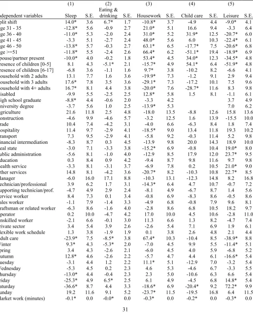
TABLE 5—TIME USE ESTIMATIONS (MINUTES). FEMALE FULL-TIME WAGE EARNERS. OLS ESTIMATES (1) (2) (3) (4) (5)
Independent variables Sleep S.E.
Eating &
drinking S.E. Housework S.E. Child care S.E. Leisure S.E.
Split shift 14.0* 3.6 6.7* 1.7 -10.8* 3.7 -4.9 4.4 -9.0* 4.1
Age 31 - 35 -12.8* 5.6 -0.9 2.7 21.0* 5.1 16.6 9.4 -3.3 6.4
Age 36 - 40 -11.0* 5.3 -2.0 2.4 31.0* 5.2 31.9* 12.5 -20.7* 6.0
Age 41 - 45 -3.3 5.1 -2.7 2.4 48.0* 5.6 6.0 10.3 -22.4* 6.1
Age 46 - 50 -13.8* 5.7 -0.3 2.7 63.1* 6.5 -17.7* 7.5 -20.6* 6.8
Age >=51 -11.8* 5.5 -2.4 2.6 66.4* 6.2 -51.1* 19.4 -18.9* 6.9
Spouse/partner present -10.0* 4.0 -0.2 1.8 53.4* 4.5 34.0* 12.3 -34.5* 4.8
Presence of children [0-5] 8.1 4.3 -5.1* 2.1 -15.7* 4.9 54.1* 6.4 -51.9* 4.8
Presence of children [6-17] -6.8 3.6 -1.1 1.6 9.7* 3.8 -10.2 8.2 -6.6 4.1
Household with 2 adults 13.1 7.7 1.6 3.6 -19.9* 7.3 -1.2 9.1 2.9 9.4
Household with 3 adults 17.6* 7.8 3.5 3.6 -29.1* 7.3 -17.2 10.1 7.5 9.6
Household with 4+ adults 16.7* 8.1 4.4 3.8 -20.0* 7.6 -28.7* 11.6 8.3 9.8
Disabled -9.9 5.5 -2.5 2.5 12.8* 5.8 1.5 8.1 -1.1 6.1
High school graduate -8.8* 4.4 -0.6 2.0 -3.3 4.2 3.7 4.9
University degree -3.7 5.6 1.0 2.5 -13.9* 5.3 7.0 6.2
Agriculture 21.6 11.8 2.5 4.8 -18.0 13.5 -8.8 12.6 15.8 13.6
Construction -4.6 9.9 -4.6 5.7 -3.2 12.5 1.6 13.9 -15.5 10.0
Trade 10.4 7.4 -4.2 3.1 -4.0 6.6 -6.3 8.4 1.8 7.4
Hospitality 11.4 9.7 -2.9 4.1 -18.5* 9.0 13.4 11.8 19.3 10.2
Transport 7.3 9.5 -2.9 4.1 -5.8 9.2 -0.3 11.4 5.2 9.8
Financial intermediation -8.3 8.7 0.3 4.5 -13.9 9.8 20.0 14.3 18.9 10.0
Real state -3.0 7.1 -3.3 3.8 -15.2* 6.9 -0.8 10.4 19.0* 8.0
Public administration -5.6 8.1 -1.0 4.0 -12.9 8.5 17.9 12.0 23.7* 9.5
Education 0.3 8.4 0.9 4.2 -9.4 8.7 9.8 11.6 9.7 9.8
Health service -3.3 8.1 -3.1 3.7 -6.9 7.8 0.2 10.5 21.0* 9.0
Other services 14.8 8.1 -4.2 3.6 -20.7* 8.2 -10.3 10.8 22.7* 8.5
Manager -6.0 16.0 17.1 8.8 -10.3 13.1 -12.3 14.8 8.2 16.8
Technician/professional 3.9 6.2 1.7 3.1 -14.3* 6.4 4.7 10.7 -0.7 7.2
Supporting technician/prof. -4.7 4.9 2.9 2.4 -8.1 4.9 -6.7 8.7 1.4 5.6
Service worker 8.4 7.3 0.1 3.4 -0.8 6.9 -8.3 8.6 -0.5 8.6
Sales worker -1.1 7.9 -1.4 3.3 -4.9 6.8 -0.8 7.9 9.6 8.1
Craftsman or related worker -6.3 8.6 -1.6 4.0 -2.8 8.6 6.8 10.5 18.2 9.7
Operator 0.2 10.0 -4.7 4.2 17.0 10.0 4.5 10.6 -2.8 11.0
Unskilled worker -2.1 6.6 -0.1 3.0 11.3 6.6 1.3 8.2 -4.7 7.4
Private sector 3.4 5.4 3.9 2.6 -2.6 5.4 7.1 6.9 1.9 6.1
Flexible work schedule 1.3 3.8 -1.9 1.9 0.1 3.8 2.6 4.8 2.1 4.4
Adult care -23.9* 7.5 -8.5* 3.8 67.4* 10.3 -10.4 8.5 -38.9* 8.8
Winter 9.3* 4.3 -5.3* 2.0 -7.0 4.5 9.9 5.5 -11.4* 5.1
Spring 3.4 4.3 -2.6 2.1 -6.0 4.5 4.0 5.9 -6.8 5.2
Autumn 12.8* 4.6 -2.6 2.2 -5.7 4.7 4.4 6.1 -16.6* 5.4
Tuesday -3.1 4.4 1.2 2.2 11.1* 5.1 -12.9 7.0 -3.2 5.4
Wednesday -5.3 4.5 0.2 2.3 4.6 5.3 -4.6 6.7 -3.3 5.5
Thursday -13.0* 4.4 -0.4 2.3 2.3 5.0 -10.6 6.3 6.6 5.4
Friday -25.3* 4.9 6.5* 2.5 6.1 4.9 -4.5 6.8 14.8* 5.4
Saturday -36.6* 8.7 4.4 3.3 -18.6* 6.9 -20.4* 9.2 72.2* 9.9
Sunday 19.2 11.6 9.1 5.2 -23.7* 11.5 -19.5 16.8 6.4 11.5
32
Income <500 18.6 17.5 -2.9 9.7 23.1 21.6 -18.1 22.2 -26.9 21.0
Income 500 - 999.99 -5.0 10.6 -14.0* 5.9 23.3* 11.0 -8.2 14.4 6.0 11.6
Income 1000 - 1499.99 2.8 9.3 -6.9 5.6 15.5 10.0 -10.7 14.1 -0.2 9.9
Income 1500 - 1999.99 2.0 8.9 -10.4 5.4 26.9* 9.6 -9.3 13.7 -9.6 9.3
Income 2000 - 2499.99 5.5 8.9 -11.1* 5.3 18.8 9.7 1.5 13.3 -6.2 9.2
Income 2500 - 2999.99 -4.2 8.8 -9.9 5.5 14.5 9.9 -7.3 12.9 6.8 9.6
Income 3000 - 4999.99 -5.4 8.7 -9.9 5.3 11.7 9.6 8.4 11.9 9.2 9.1
Inverse Mills ratio 42.3 22.6
Intercept 499.0* 18.5 107.4* 8.9 244.8* 18.2 51.9 28.7 298.8* 20.4
R-squared 0.091 0.045 0.409 0.408 0.234
Observations 2,596 2,596 2,596 1,065 2,596
Notes: Standard errors are robust to heteroskedasticity, but those pertaining to estimation (4) have been additionally
corrected for the presence of generated regressors. Unreported categories: Age <=30, 1-adult household, less than high
school graduate, manufacturing, clerical worker, summer, Monday, and household income >=5,000. *: Significant at 5
33
TABLE 6—TIME USE ESTIMATIONS (MINUTES). MALE FULL-TIME WAGE EARNERS. OLS ESTIMATES (1) (2) (3) (4) (5)
Independent variables Sleep S.E.
Eating &
drinking S.E. Housework S.E. Child care S.E. Leisure S.E.
Split shift 10.2* 2.8 5.9* 1.3 -9.6* 2.0 -8.7* 2.7 -9.1* 3.2
Age 31 - 35 13.0* 4.5 2.7 2.1 4.8 3.0 0.1 5.5 -10.1* 5.1
Age 36 - 40 -2.9 4.6 0.9 2.2 4.2 3.2 15.2 8.4 -3.6 5.6
Age 41 - 45 -1.1 4.6 0.1 2.3 7.6* 3.5 5.3 8.6 0.7 5.5
Age 46 - 50 12.0* 4.5 3.3 2.4 14.0* 3.9 -9.5 5.7 -6.9 5.7
Age >=51 9.1* 4.3 1.1 2.1 1.7 3.6 -49.9* 17.6 13.9* 5.4
Spouse/partner present -0.9 3.7 2.3 1.9 15.7* 3.0 62.4* 22.0 -28.5* 4.6
Presence of children [0-5] -3.2 3.3 -4.7* 1.7 -4.2 2.8 21.5* 3.2 -24.7* 4.1
Presence of children [6-17] 1.1 2.6 0.1 1.3 -5.9* 2.1 -15.8* 4.3 -1.5 3.3
Household with 2 adults 18.8* 9.0 -5.4 4.3 -30.3* 5.7 54.0 28.4 31.0* 9.4
Household with 3 adults 22.5* 8.9 -3.1 4.3 -41.1* 5.5 41.0 27.2 33.3* 9.3
Household with 4+ adults 28.6* 9.0 -5.4 4.4 -49.0* 5.5 32.5 24.1 40.5* 9.4
Disabled -0.3 3.9 -2.1 1.8 6.5* 3.2 -4.5 4.2 -5.7 4.9
High school graduate -3.5 3.0 -3.7* 1.4 5.8* 2.1 2.6 3.5
University degree -10.1* 4.4 -5.8* 2.2 4.9 3.7 -3.4 5.6
Agriculture 12.9* 6.5 3.5 3.0 -11.8* 4.0 -12.4* 5.5 -0.5 7.2
Construction -7.2* 3.5 8.0* 1.8 -9.7* 2.4 -2.7 3.4 -8.9* 4.1
Trade -1.0 4.3 -2.7 2.1 -8.6* 3.0 -4.6 4.4 14.2* 5.3
Hospitality 13.4 9.5 -6.2 4.5 -11.9 7.4 -1.7 9.0 -3.0 10.2
Transport -1.4 4.8 4.6 3.0 -10.2* 4.0 -1.9 5.5 3.8 6.8
Financial intermediation -9.1 6.4 1.5 3.6 -19.1* 5.2 -5.2 6.9 19.2* 8.6
Real state 0.2 6.0 0.3 2.8 -2.9 4.6 -6.9 7.9 6.1 7.5
Public administration 8.5 6.5 -0.3 3.0 -0.5 5.5 -5.6 7.3 8.2 8.4
Education 15.3* 7.3 0.6 3.7 -4.2 6.2 -6.8 10.0 -7.2 9.9
Health service 20.7* 9.9 -1.9 3.8 0.1 7.4 -0.4 10.4 -12.6 10.3
Other services 10.8 8.5 -0.2 3.5 -12.0 6.2 -16.7* 7.1 7.0 10.7
Manager 5.2 7.8 5.4 4.2 -13.5* 6.7 -15.8 8.2 4.2 10.1
Technician/professional 1.7 6.3 2.2 3.2 -10.7 6.1 -2.0 7.9 8.6 8.4
Supporting technician/prof. -1.9 5.5 -2.5 2.7 -3.8 5.0 -6.2 7.0 9.6 7.2
Service worker -0.2 7.6 -3.9 3.4 -1.6 6.9 -11.8 8.1 11.9 9.4
Sales worker 12.8 8.5 -0.1 4.1 10.1 6.6 -12.4 8.8 -9.0 9.9
Craftsman or related worker 11.6* 5.4 -3.7 2.6 -5.6 4.6 -13.9* 6.5 8.3 6.8
Operator 12.5 6.5 -1.3 2.9 -6.4 5.0 -18.9* 6.8 6.7 7.6
Unskilled worker 9.3 6.1 -1.3 2.9 -1.8 5.0 -10.0 7.3 0.4 7.7
Private sector 4.9 4.7 0.8 2.3 0.2 3.7 -7.4 5.2 1.3 6.1
Flexible work schedule 7.8* 2.8 1.1 1.5 -3.7 2.3 -2.0 3.3 1.1 3.5
Adult care -24.4* 7.5 -10.5* 4.0 80.3* 13.5 -38.3* 11.5 -24.3* 9.7
Winter 4.1 3.3 -1.5 1.6 -5.1* 2.5 4.0 3.6 -10.0* 4.0
Spring -0.9 3.3 -2.3 1.6 -0.1 2.6 1.1 3.4 -2.2 4.1
Autumn 1.0 3.4 -2.9 1.7 -1.1 2.7 8.0* 3.6 -8.1 4.4
Tuesday -6.0 3.4 -1.0 1.7 -4.9 2.9 -4.1 3.8 0.8 4.3
Wednesday -3.6 3.5 0.8 1.8 0.9 3.0 -3.8 4.2 -2.5 4.4
Thursday -7.7* 3.6 -2.1 1.8 -2.2 3.0 0.9 4.2 6.1 4.7
Friday -26.6* 3.7 4.8* 1.8 1.7 2.9 0.7 3.8 16.6* 4.4
Saturday -34.3* 8.0 4.4 3.2 -3.6 4.9 -3.3 5.9 50.2* 8.9
Sunday 27.6* 10.7 5.8 5.2 -19.7* 6.8 -9.2 10.3 6.1 12.5
34
Income <500 46.6 27.7 -4.6 6.5 -27.6* 12.4 -16.2 17.1 -39.1* 18.5
Income 500 - 999.99 -3.4 8.0 -1.5 4.6 -22.1* 7.7 -7.1 8.0 3.6 10.8
Income 1000 - 1499.99 -1.6 7.4 -1.0 4.3 -18.9* 7.4 -8.1 8.0 0.2 10.0
Income 1500 - 1999.99 -5.7 7.2 0.1 4.3 -7.6 7.3 -3.2 7.9 -5.9 9.9
Income 2000 - 2499.99 -6.5 7.3 1.7 4.3 -8.4 7.4 1.7 7.7 -7.2 10.0
Income 2500 - 2999.99 -4.9 7.4 -2.8 4.4 -1.3 7.5 0.0 9.2 -12.4 10.1
Income 3000 - 4999.99 -13.4 7.4 1.9 4.4 -4.6 7.2 3.0 8.0 -3.3 10.0
Inverse Mills ratio 51.8* 25.1
Intercept 483.0* 16.2 106.4* 7.8 178.9* 13.3 -44.5 62.7 378.0* 18.6
R-squared 0.075 0.039 0.207 0.268 0.250
Observations 4,204 4,204 4,204 1,933 4,204
Notes: Standard errors are robust to heteroskedasticity, but those pertaining to estimation (4) have been additionally
corrected for the presence of generated regressors. Unreported categories: Age <=30, 1-adult household, less than high
school graduate, manufacturing, clerical worker, summer, Monday, and household income >=5,000. *: Significant at 5
35
FIGURE 1. FRACTION AT WORK ON A REGULAR WORKING DAY. MALE AND FEMALE FULL-TIME WAGE EARNERS.
36
FIGURE 2. EFFECT OF BEING ON A SPLIT SHIFT ON TIME SPENT SLEEPING ON REGULAR WORKING DAYS, BY TIME OF DAY AND SEX.
Notes: Author’s calculations with data on full-time wage earners taken from the Spanish Time Use Survey 2002-2003. The effects represented are those achieving statistical
37
FIGURE 3. EFFECT OF BEING ON A SPLIT SHIFT ON TIME SPENT EATING ON REGULAR WORKING DAYS, BY TIME OF DAY AND SEX.
Notes: Author’s calculations with data on full-time wage earners taken from the Spanish Time Use Survey 2002-2003. The effects represented are those achieving statistical