Unsupervised Text Normalization Using Distributed Representations of
Words and Phrases
Vivek Kumar Rangarajan Sridhar∗ AT&T Labs - Research
1 AT&T Way, Bedminster, NJ 07920
Abstract
Text normalization techniques that use rule-based normalization or string similar-ity based on static dictionaries are typ-ically unable to capture domain-specific
abbreviations (custy, cx→customer) and
shorthands (5ever, 7ever→forever) used
in informal texts. In this work, we ex-ploit the property that noisy and canoni-cal forms of a particular word share simi-lar context in a simi-large noisy text collection (millions or billions of social media feeds from Twitter, Facebook, etc.). We learn distributed representations of words to capture the notion of contextual similarity and subsequently learn normalization lex-icons from these representations in a com-pletely unsupervised manner. We experi-ment with linear and non-linear distributed representations obtained from log-linear models and neural networks, respectively. We apply our framework for normalizing customer care notes and Twitter. We also extend our approach to learn phrase
nor-malization lexicons (g2g→got to go) by
training distributed representations over compound words. Our approach outper-forms Microsoft Word, Aspell and a man-ually compiled urban dictionary from the Web and achieves state-of-the-art results on a publicly available Twitter dataset.
1 Introduction
Text normalization is a prerequisite for a variety of tasks involving speech and language. Most natu-ral language processing (NLP) tasks require a tight and compact vocabulary to reduce the model com-plexity in terms of feature size. As a consequence, applications such as syntactic tagging and parsing, semantic tagging, named entity extraction, infor-mation extraction, machine translation, language ∗The author is currently with Apple, Inc., and can be
contacted at [email protected].
models for speech recognition, etc., are trained on clean data that is normalized and restricted to some user defined vocabulary. Conventionally, most NLP researchers perform such normalization through rule-based mapping that can get unwield-ily and cumbersome for extremely noisy texts as in SMS, chat or social media.
Unnormalized text, as witnessed in social me-dia forums such as Facebook, Twitter and message boards, or short messaging service (SMS), have a variety of issues with spelling that include re-peating letters, eliminating vowels, using phonetic spellings, substituting letters (typically syllables) with numbers, using shorthands and user created abbreviations for phrases. The remarkable prop-erty of such texts is that new variants of canonical
words and phrases evolve constantly (e.g.,jghome
→ just got home). Hence, it is important to de-sign a framework that can learn the mapping be-tween unnormalized and canonical forms of such words and phrases in an unsupervised and exten-sible manner.
Conventional edit distance (Levenshtein, 1966) based approaches are not accurate for predicting spelling correction for large number of edits in abbreviations and shorthands found in informal texts. In this work, we exploit the property that noisy and canonical forms of a particular word share similar context in a large noisy text collec-tion (millions or billions of social media feeds from Twitter, Facebook, etc.). We represent the words in a vector space using distributed repre-sentations to capture the notion contextual similar-ity and subsequently learn normalization lexicons from these representations. The distributed repre-sentations are induced either through neural net-works (non-linear embeddings) or log-linear mod-els (linear embeddings). The proposed approach uses the property of contextual similarity between canonical and noisy versions of a particular word
to cluster them in RD, where D is the
dimen-sion of the distributed representation. We also extend our framework to learn one-to-many
map-pings (e.g., ily→i love you,nbd→no big deal
by learning distributed representations over words and phrases.
We demonstrate the fidelity of our approach on customer care domain and Twitter. We also compare our approach with Microsoft Word, As-pell, custom dictionaries compiled from the Web as well as state-of-the-art techniques for unsuper-vised normalization.
2 Related Work
Text normalization has been traditionally per-formed in a task specific manner through string edit operations. While a large proportion of NLP researchers still perform this exercise manually by writing regular expression patterns, several auto-matic procedures have been proposed. A sim-ple way to perform this string edit operation is by using a noisy channel model (Brill and Moore, 2000). However, this requires supervised training data in the form of the canonical and erroneous strings. Since words are spoken using phonet-ics, it is instructive to look at the problem from the point of pronunciation changes. For exam-ple, (Toutanova and Moore, 2002) extended the noisy channel framework to include word
pronun-ciation information. Theaspelltool for spelling
correction also works on a phonetic algorithm for string normalization (Philips, 1990).
(Cook and Stevenson, 2009) introduced an un-supervised noisy channel model that considered several word formation processes in a generative model. Another popular way to normalize or even punctuate text is by using phrase-based machine translation. (Aw et al., 2009) used a character level phrase-based machine translation approach to translate SMS text into clean English text. How-ever, such an approach still requires supervised training data. Furthermore, noisy channel mod-els typically do not use wider context in resolving the normalization problem. Clearly, many of the unnormalized forms appear in the same context as the canonical form and exploiting such informa-tion is critical.
Social media text normalization using contex-tual graph random walks was recently proposed in (Hassan and Menezes, 2013). They use a lexi-con based approach where the normalization lex-icon is obtained in an unsupervised manner by performing random walks on contextual
similar-ity graphs (bipartite) constructed fromn-gram
se-quences. A similar approach using distributional
similarity was also proposed in (Han et al., 2012a) where a pairwise similarity deems two words with identical context to be normalization equivalences. Due to the pairwise computation, it does not result in a globally optimized equivalence. Our frame-work is most similar to (Hassan and Menezes, 2013) as we also use the notion of distributional similarity between strings at a corpus level to iden-tify normalization equivalences in an unsupervised manner. In contrast, we use distributed representa-tion of words to capture contextual similarity and learn unsupervised lexicons using both lexical and vector space feature functions. The proposed ap-proach is relatively simple, scalable and easily re-producible.
3 Distributed Representation of Words
Conventional NLP applications typically use one-hot encoding where each word in the vocabulary is represented by a bit vector. Such a represen-tation exacerbates the data sparsity problem and does not exploit any semantic or syntactic rela-tionship that may be present amongst subset of words. Distributed representation of words (also called word embeddings or continuous space rep-resentation of words) has become a popular way for capturing distributional similarity (lexical, se-mantic or even syntactic) between words. The
ba-sic idea is to represent each wordwi∈V with a
real-valued vector of some fixed dimensionD, i.e.,
wi ∈ RD ∀ i = 1,· · ·, V. The idea of
repre-senting words in vector space was originally pro-posed in (Rumelhart et al., 1986; Elman, 1991). However, improved training techniques and tools in the recent past have made it possible to obtain such representations for large vocabularies.
Distributed representations can be induced for a
given vocabulary V in several ways. While they
un-wt 2
wt 1
wt+1
wt+2
wt {forever, 5ever, 4ever, forevr}
{took,love} {you,me} {to,with} {go,heart}
Projection
(a) Continuous Bag-of-Words Architecture
Lookup Table d
d*5 (concatenation)
Linear
Tanh
Linear
Lookup Table d
d*5 (concatenation)
Linear
Tanh Linear
love you forever with heart love you example with heart took you 4ever to go took you washington to go
f✓(s) f✓(sc)
Loss = max(0,1 f✓(s) +f✓(sc))
[image:3.612.124.495.66.211.2](b) Neural Network Architecture
Figure 1: Illustration of obtaining distributed representations for text normalization using two different approaches
supervised manner.
Figure 1 shows two different architectures for inducing distributed representations. On the left side, the architecture for the continuous bag-of-words model (Mikolov et al., 2013) is shown while the neural network learning architecture for induc-ing distributed representations in language mod-els (Collobert and Weston, 2008) is shown on the right. Both these frameworks essentially perform a similar function in that the word representations are created based on contextual similarity. Fig-ure 1 also shows an example of the contextual sim-ilarity that can be exploited such that canonical and noisy versions of a particular word have sim-ilar vector representation (in terms of some
simi-larity metric). It is shown that the words{forever,
4ever, 5ever, forevr}share similar context. It is
also interesting to note that the word5everthat is
used to meanlonger than 4evercan be identified
to meanforeverthat edit distance matching is
typ-ically not able to capture.
Language
en
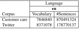
[image:3.612.131.270.538.589.2]Corpus Vocabulary #Sentences Customer care 7846840 870491324 Twitter 8371078 178770137
Table 1: Statistics of the data used to learn dis-tributed representations
4 Data
We use two sources of data in our work. One is internal anonymized customer care notes and the other is Twitter. The customer care data refers to notes made by agents at mobility call centers when
customers make a call. Each call typically results in one record and the notes typically consist of a brief summary of the call from the representative side. The data we use does not contain any meta-data beyond the text description. We used all the data between Dec 2012 and Jan 2014. The text data is extremely noisy as the agents are making these notes either during their interaction or imme-diately afterward. Hence, the data contains several spelling errors and abbreviations that need to be corrected before performing any large scale data analytics.
We also acquired a 10% random sample of Twitter firehose data across all languages. As a first step, we filtered the tweets by language code. Since the language code is a property set in the user profile, the language code does not guarantee that all tweets are in the same language. We used a simple frequency threshold for language iden-tification based on language specific word lists. Subsequently, we performed some basic clean-up such as replacing usernames, hashtags, web ad-dresses and numerals with generic symbols such as user, hashtags , url and number. Finally, we removed all punctuations from the strings and lowercased the text. In this work, we perform our experiments on English.
5 Training Distributed Representations
with 100 nodes and a linear layer with one output. However, we used a right and left context of 5 (or 7) words and corrupted the centre word instead of the last word to learn the distributed
representa-tions. Given a text windows ={w}wlen
1 ,wlen1
is the window length, and a set of parameters
as-sociated with the networkθ, the network outputs
a scorefθ(x). The approach then minimizes the
ranking criterion with respect toθsuch that:
θ7→X
s∈X
X
w∈V
max{0,1−fθ(s) +fθ(sc)} (1)
whereX is the set of all windows of lengthwlen
in the training data, V is the vocabulary and sc
denotes the corrupted version ofs with the
mid-dle word replaced by a random word w in V.
We used a frequency threshold of 10 occurrences for the centre word, i.e., all words below this frequency was not considered in training. We performed stochastic gradient minimization over 1000 epochs on each dataset and used the Torch toolkit (Collobert et al., 2011) to train the repre-sentation.
We also used a log-linear model for inducing the distributed representations using the continuous-bag-of-words architecture proposed in (Mikolov
et al., 2013). The continuous-bag-of-words
model is similar to the neural network language model (Bengio et al., 2003) with the non-linear layer replaced by a sum pooling layer, i.e., the model uses a bag of surrounding words to pre-dict the centre word. Since the implementation of this architecture was readily available through the
word2vec tool2, we used it for inducing the
repsentations. We used hierarchical sampling for re-ducing the vocabulary during training and used a minimum count of 10 occurrences for each word.
The framework presented in this paper can also work with word vectors obtained using other tech-niques such as latent semantic indexing, convolu-tional neural networks, recurrent neural networks, etc.
6 Learning Normalization Lexicons
Once we obtain the set of word embeddings
wi 7→ di, ∀i ∈ V;di ∈ RD, our
frame-work requires a list of canonical words as in-put. For English, we used a wordlist from Project
1wlenin our work is an odd number, e.g.,wlen= 11
implies a left and right context of5words
2https://code.google.com/p/word2vec/
Gutenberg (http://www.gutenberg.org/
ebooks/3201) consisting of 113809 words.
Given a canonical words1, we find theK-nearest
neighbors in the vector space and objectively
mea-sure the similarity betweens1and the neighbors,
i.e., from each pair of stringss1ands2with
cor-responding vectorsuandv, we obtain lexical and
vector space features described below.
6.1 Similarity Cost
The cosine distance between twoD-dimensional
vectorsuandvis defined as,
cosine similarity=
D
P
i=1ui×vi s
D
P
i=1(ui) 2×PD
i=1(vi) 2
(2) The lexical similarity cost is computed similar to that presented in (Hassan and Menezes, 2013).
lexical similarity(s1,s2) =LCSRED(s1(s1,s2,s2))
(3)
LCSR(s1,s2) =Max LengthLCS(s1,(s2s1),s2) (4)
where LCSR refers to the Longest Common Sub-sequence Ratio (Melamed, 1995), LCS refers to Longest Common Subsequence and ED refers to the edit distance between the two strings. For English, the edit distance computation was mod-ified to find the distance between the consonant
skeleton of the two stringss1 ands2, i.e., all the
vowels were removed. Repetition in the strings was reduced to a single letter and numbers in the words were substituted by their equivalent letters. The general algorithm for learning a normalization lexicon through our approach is presented in Al-gorithm 1. While it is possible to learn optimal weights for several feature functions through min-imum error rate training (Och, 2003), we use uni-form weights in the absence of a significant held-out set for optimization.
6.2 Representation of Lexicons using FSTs
We compile the lexicon L obtained using
0/0 adavised:advised/-9999
adbised:advised/-0.87 adbised:advise/-0.49 adised:advised/-0.88 adivced:advised/-0.75 csuotmer:customer/-9999 csustomer:customer/-9999cuostmer:customer/-9999 cusst:customer/-0.41 custy:customer/-0.42 cux:customer/-0.29 <unknown>:<unknown>/0
°
°
LM)adavised cux to call hotline
advised customer to call hotline bestpath( input fsm
1.38 0.86 0.89 -13.8 -13.8 -13.8 0.28
[image:5.612.136.485.66.170.2]-13.8 0.12 0.71 0.14
Figure 2: Illustration of the normalization technique using finite state transducers. The unknown words in the input are preserved in the output.
Algorithm 1Unsupervised Lexicon Learning
input {di}|iV=1|: distributed representation of
words for vocabulary|V|
inputK: number of nearest neighbors
inputCOST: lexical similarity metric
inputW: list of canonical words
foreachw∈Wdo foreachi∈ |V|do
if wi7→di∈/Wthen
Compute cosine distance between di
andd(w)
Store topKneighbors in mapL(w)
foreachw∈Wdo foreacho∈L(w)do
ComputeCOST(w,o)
Pushw7→ {o,COST(w,o)}intoD
Invert the mapDto obtain lexiconL
The normalization lexicon is converted into a sgle state finite-state transducer (FST) with the in-put and outin-put labels being the noisy and canoni-cal word, respectively. In all our experiments, we
used the number of nearest neighborsK= 25.
Given a sentence that needs to be normalized,
we form a linear FSMsfrom the text string and
compose it with the FST lexiconN. The
result-ing FSM is then composed with a language model
(LM)L, if available, and the best path is found
to obtain snorm. We used a trigram language
model that was trained on a variety of texts (En-glish Gigaword, Web, Opensubtitles, etc.). We used Kneser-Ney discounting and the LM was not optimized in any way.
snorm=bestpath(s◦N◦L) (5)
Figure 2 illustrates this procedure. The unknown words in the input are preserved in the output (the
language model is trained with an open vocabu-lary).
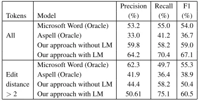
6.3 Evaluation
First, we evaluated our approach on customer care data. A set of 300 sentences from the customer care data was randomly selected and the refer-ence sentrefer-ences were created manually by a pro-fessional transcriber. A total of 2387 tokens were normalized by the transcribers. The distributed representation was trained on the remaining cus-tomer care data through neural network learning approach (Collobert and Weston, 2008) over a window of 11 words with a vector dimension of 100. We compare our approach with Microsoft Word and Aspell, where the best option was man-ually chosen (oracle) from the suggestion list. If no option was appropriate, the word was left in it’s original form. We measure the fidelity of nor-malization using precision and recall. The results are presented in Table 2.
Precision Recall F1 Tokens Model (%) (%) (%)
[image:5.612.317.515.500.601.2]Microsoft Word (Oracle) 53.2 55.0 54.0 All Aspell (Oracle) 33.0 41.2 36.7 Our approach without LM 59.8 58.2 59.0 Our approach with LM 64.2 70.4 67.1 Microsoft Word (Oracle) 62.3 49.7 55.3 Edit Aspell (Oracle) 41.9 36.4 38.9 distance Our approach without LM 44.4 58.2 50.4 >2 Our approach with LM 50.61 75.1 60.5
Table 2: Sentence level normalization on customer care notes
Category Model Precision (%) Recall (%) F1 (%) Microsoft Word (Oracle) 72.7 30.8 43.3 Aspell (Oracle) 83.0 35.4 49.6 Web dictionary with LM 79.8 24.2 37.1 Neural Network (wlen:11+D:100) lexicon without LM 53.4 74.7 62.3 Neural Network (wlen:11+D:100) lexicon with LM 54.4 77.1 63.8 Word Neural Network (wlen:11+D:200) lexicon with LM 50.5 75.1 60.4 Neural Network (wlen:15+D:100) lexicon with LM 54.2 73.5 62.4 Neural Network (wlen:15+D:200) lexicon with LM 48.5 75.4 59.0 Log-Linear Model (wlen:11+D:100) lexicon with LM 54.5 77.2 63.9 Log-Linear Model (wlen:11+D:200) lexicon with LM 51.2 75.9 61.1 Log-Linear Model (wlen:15+D:100) lexicon with LM 54.6 76.1 63.5 Log-Linear Model (wlen:15+D:200) lexicon with LM 47.1 75.1 57.9
Table 3: Sentence level word normalization on English Twitter data
to note that while our approach is customized to the domain, the baseline comparisons are not. The performance for noisy words that differ in edit dis-tance by more than 2 from the canonical word is also shown in Table 2. Our framework achieves significantly better performance for abbreviations
that typically have edit distance>2. Since our
ap-proach combines the strength of distributional and lexical similarity as opposed to most approaches that rely only on string similarity, we are also able to correctly normalize domain specific
abbrevia-tions, e.g.,custy→customer,cx→customer,lqd
→ liquid, bal → balance, exp → expectations, etc. The use of a language model significantly im-proves the normalization accuracy.
We also performed sentence (tweet) level nor-malization on Twitter data. We manually an-notated (expanded abbreviations, shorthands and spelling errors) 1000 tweets and performed nor-malization using our approach. The annotation was performed serially by two professional tran-scribers. We compare our approach with Mi-crosoft Word, Aspell and a dictionary compiled from several websites. We use a log-linear model (continuous-bag-of-words) as well as a neural net-work (see Section 5) to automatically learn nor-malization lexicons. For each model, we
experi-mented with window length (wlen) of 11 and 15
while the dimension of distributed representation was either 100 or 200. The results in Table 3 indi-cate that using Algorithm 1 we achieve impressive performance with both models in comparison with the other schemes. The log-linear model works just as well as the non-linear model and is much quicker to train. One should note that the results from Microsoft Word and Aspell overestimate the fidelity of normalization since the task was per-formed manually, i.e., we picked the best option
from the suggestion list. In case of no correct sug-gestion, we left the original form as is. Hence, the results are skewed towards achieving high preci-sion. In contrast, our approach is completely un-supervised in design and evaluation. We also com-pared our approach with a Twitter and SMS nary compiled from several websites. The dictio-nary contained entries for 3864 words and 3536 phrases. The dictionary was compiled into a FST and the procedure in Section 6.2 was used for eval-uation. Since, the dictionary entries do not have an
associated score, the FST lexiconNis unweighted.
Our results clearly indicate that for construction of the normalization lexicon all we need is a reliable distributed representation trained on large amount of noisy text. The non-linearity with the neural network does not help significantly for this task.
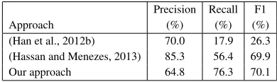
Precision Recall F1
Approach (%) (%) (%)
(Han et al., 2012b) 70.0 17.9 26.3 (Hassan and Menezes, 2013) 85.3 56.4 69.9 Our approach 64.8 76.3 70.1
Table 4: Sentence level normalization on Twitter test set from (Han et al., 2012b)
[image:6.612.318.513.458.516.2]Category Model Precision (%) Recall (%) F1 (%) Microsoft Word (Oracle) 99.2 18.7 31.5 Aspell (Oracle) 75.0 0.4 0.8 Web dictionary with LM 34.0 19.0 24.4 Neural Network (wlen:11+D:100) without LM 91.4 60.7 73.0 Neural Network (wlen:11+D:100) with LM 92.4 71.3 80.5 Phrase Neural Network (wlen:11+D:200) lexicon with LM 92.5 71.8 80.8 Neural Network (wlen:15+D:100) lexicon with LM 92.4 71.4 80.6 Neural Network (wlen:15+D:200) lexicon with LM 92.5 71.8 80.8 Log-Linear Model (wlen:11+D:100) lexicon with LM 92.6 72.0 81.0 Log-Linear Model (wlen:11+D:200) lexicon with LM 92.3 71.1 80.3 Log-Linear Model (wlen:15+D:100) lexicon with LM 92.6 71.5 80.6 Log-Linear Model (wlen:15+D:200) lexicon with LM 92.0 70.9 80.0
Table 5: Sentence level phrase normalization on English Twitter data
7 Learning Phrase Normalizations
A major drawback of inducing normalization lex-icons using most approaches described in Sec-tion 2 is that they are restricted to learning one-to-one word mappings. However, social media text is strewn with abbreviations that span
multi-ple words, e.g.,ily2refers toi love you too. With
our framework, one can obtain 1-to-many (or vice versa) mappings if the training data is modified
to contain compound words, i.e.,i love you toois
replaced withi love you tooand treated as a
sin-gle token. The biggest obstacle is to get a reli-able list of such phrases since they keep changing and growing. Unsupervised phrase induction us-ing likelihood ratio test, point-wise mutual infor-mation, etc., may be used for such a task but they typically do not capture phrases formed from high frequency function words.
We used a dataset of speech-based SMS mes-sage transcriptions for compiling a list of com-mon phrases. The SMS messages were collected through a smartphone application and a majority of them were collected while the users used the application in their cars. We had access to a to-tal of 41.3 million English messages. The speech transcripts were mostly automatic and only a sub-set of around 400K utterances were manually tran-scribed. To avoid the use of erroneous transcripts, we sorted the messages by frequency and picked phrases between length 2 and 4 that resulted in 27356 English phrases. The training data was then phrasified (words were compounded) with the above phrase lists and the experiments to learn distributed representations was repeated. We per-formed this experiment only on Twitter data.
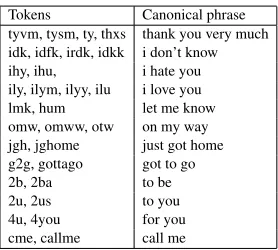
Once the representations were learned, we com-puted the K-nearest neighbors using the cosine
Tokens Canonical phrase tyvm, tysm, ty, thxs thank you very much idk, idfk, irdk, idkk i don’t know ihy, ihu, i hate you ily, ilym, ilyy, ilu i love you lmk, hum let me know omw, omww, otw on my way jgh, jghome just got home g2g, gottago got to go 2b, 2ba to be 2u, 2us to you 4u, 4you for you cme, callme call me
Table 6: Phrase normalizations learned through our framework
similarity metric for each phrase. The
lexi-cal similarity cost was computed differently for the phrases. The first character of each word in the phrase was picked to form a new string
(e.g.,i love you toowould be converted intoilyt)
and a similar technique was used on the nearest neighbors; singleton numbers were expanded into
strings (e.g., ily2 would be converted into ilyt).
The lexical similarity metric in Equation (3) was then used to compute the distance between the two strings. The normalization table was subse-quently inverted and compiled into a FST. Table 6 shows some of the phrase normalizations learnt by our framework. The phrase normalization results for English are presented in Table 5. Our frame-work learns phrase normalizations quite well. We achieve precision and recall of 92.6% and 72.0%, respectively. Even the mistakes committed are not
very different from the ground truth, e.g., idk→
i do not knowwhile the reference isi don’t know,
wtf →what the hellinstead ofwhat the f***and
[image:7.612.347.486.235.360.2]such asnz→new zealand,la→los angelesand some highly context dependent expansions such asdw→doctor who,dm→direct message, etc., since the compiled phrase list did not contain these entries.
8 Discussion
The normalization lexicons learned in this work are completely unsupervised. The quality and cov-erage of the lexicon is dependent on the size and distribution of words in the training data. Our approach assumes that the data contains both the noisy and canonical form of a word. In practice, we have observed that for large text collections, such as millions of tweets, words appear in both canonical and noisy forms. One can also augment noisy corpora with clean text to improve the dis-tributional similarity of the two forms. Choosing the optimal size of noisy data set and appropriate augmentation is beyond the scope of this work.
The main parameters in our model arewlen,D
andK. The choice ofKis dependent on the size
of the training data, i.e., a largerKcan potentially
yield more noisy to canonical mappings. For our
datasets, the choice ofK={25,50,100}did not
result in any significant difference in performance.
Hence, we usedK = 25to increase the speed of
Algorithm 1. We also performed several
experi-ments to understand the choice of dimensionD.
In general, the choice of D is dependent on the
vocabulary size of the training data. For vocabu-lary size between 100K-500K, we found that
vec-tor dimension ofD = 50is sufficient and for
vo-cabulary size greater than1M,D = 100works
well empirically. Forwlen, a context of 5 words
to the left and right, i.e.,wlen = 11works well
and adding more context does not necessarily im-prove performance. We conjecture that this is due to the length of an average customer care note (12 words) and tweet (15 words). For datasets with
longer sentences, larger values ofwlen may be
beneficial.
The performance reported using Microsoft Word and Aspell was obtained by manually se-lecting the best suggestion. We resorted to this approach since both schemes do not provide an option to automatically normalize a document. In choosing the best suggestion option, we focused on precision, i.e., picked the best suggestion or left the original form as is. If we had forcefully picked an option from the suggestion list for all
correc-tions, the recall would have been higher at the cost of lower precision. The results using the Web dic-tionary and our unsupervised framework performs a blind evaluation.
In contrast with conventional string similar-ity based normalization schemes, our approach is good at modeling abbreviations. Abbreviations are generally hard to normalize with Levenshtein distance based approaches but the combination of distributional and lexical similarity is very help-ful in learning the mapping between abbreviated and canonical forms. In most off-the-shelf sys-tems, e.g., Microsoft Word, a standard dictionary is used and any corrections for domain specific spellings are typically performed manually. Since our scheme can be trained with raw data, we are able to address the domain specific idiosyncrasies. The word and phrase normalizations learned in this work use a particular type of lexical similarity metric. While it captures abbreviations well for English, our framework is open to the use of any linguistically motivated lexical similarity metric. Such metrics can be designed by language experts and linguistic knowledge can potentially be incor-porated into the unsupervised scheme, thus, lend-ing a way to embed llend-inguistic rules into a statistical framework.
9 Conclusion
References
A. Aw, M. Zhang, J. Xiao, and J. Su. 2009. A phrase-based statistical model for SMS text normalization. InProceedings of COLING, pages 33–40.
Y. Bengio, R. Ducharme, P. Vincent, and C. Jauvin. 2003. A neural probabilistic language model. Jour-nal of Machine Learning Research, 3:1137–1155. Y. Bengio, J. Louradour, R. Collobert, and J.
We-ston. 2009. Curriculum learning. InProceedings of ICML.
E. Brill and R. C. Moore. 2000. An improved error model for noisy channel spelling correction. In Pro-ceedings of ACL, pages 286–293.
R. Collobert and J. Weston. 2008. A unified archi-tecture for natural language processing: deep neural networks with multitask learning. InProceedings of ICML.
R. Collobert, K. Kavukcuoglu, and C. Farabet. 2011. Torch7: A matlab-like environment for machine learning. InBigLearn, NIPS Workshop.
P. Cook and S. Stevenson. 2009. An unsupervised model for text message normalization. In Proceed-ings of Workshop on Computational Approaches to Linguistic Creativity, pages 71–78.
J. L. Elman. 1991. Distributed representations, sim-ple recurrent networks, and grammatical structure. Machine Learning, 7(2-3):195–225.
B. Han, P. Cook, and Baldwin. 2012a. Automati-cally constructing a normalization dictionary for mi-croblogs. InProceedings of EMNLP, pages 421– 432.
B. Han, P. Cook, and T. Baldwin. 2012b. Automati-cally constructing a normalisation dictionary for mi-croblogs. InEMNLP-CoNLL 2012, pages 421–432. H. Hassan and A. Menezes. 2013. Social text nor-malization using contextual graph random walks. In Proceedings of ACL, pages 1577–1586.
V. I. Levenshtein. 1966. Binary codes capable of cor-recting deletions, insertions, and reversals. Soviet Physics Doklady (in English), 10(8):707710, Febru-ary.
D. Melamed. 1995. Automatic evaluation and uniform filter cascades for inducing n-best translation lexi-cons. InProceedings of the 3rd ACL Workshop on Very Large Corpora (WVLC).
T. Mikolov, S. Kopeck´y, L. Burget, J. ˘Cernock´y, and S. Khudanpur. 2010. Recurrent neural network based language model. In Proceedings of Inter-speech.
T. Mikolov, K. Chen, G. Corrado, and J. Dean. 2013. Efficient estimation of word representations in vec-tor space. InProceedings of Workshop at ICLR.
F. J. Och. 2003. Minimum error rate training in statis-tical machine translation. InProceedings of ACL. L. Philips. 1990. Hanging on the metaphone.
Com-puter Language, 7(12):39–43.
D. E. Rumelhart, G. E. Hinton, and R. J. Williams. 1986. Parallel distributed processing: Explorations in the microstructure of cognition, vol. 1. chapter Learning Internal Representations by Error Propa-gation, pages 318–362.
K. Toutanova and R. C. Moore. 2002. Pronunciation modeling for improved spelling correction. In Pro-ceedings of ACL, pages 141–151.