doi:10.4236/health.2010.27098
Statistical models for predicting number of involved
nodes in breast cancer patients
Alok Kumar Dwivedi1*, Sada Nand Dwivedi2, Suryanarayana Deo3, Rakesh Shukla1,
Elizabeth Kopras4
1Center for Biostatistical Services, Department of Environmental Health, College of Medicine, University of Cincinnati, Cincinnati,
USA; *Corresponding Author: alok_bhu1@yahoo.co.in
2Department of Biostatistics, All India Institute of Medical Sciences, New Delhi, India 3Department of Surgical Oncology, All India Institute of Medical Sciences, New Delhi, India
4Department of Environmental Health, College of Medicine, University of Cincinnati, Cincinnati, USA
Received 12 March 2010; revised 8 April 2010; accepted 10 April 2010.
ABSTRACT
Clinicians need to predict the number of invol- ved nodes in breast cancer patients in order to ascertain severity, prognosis, and design sub-sequent treatment. The distribution of involved nodes often displays over-dispersion—a larger variability than expected. Until now, the nega-tive binomial model has been used to describe this distribution assuming that over-dispersion is only due to unobserved heterogeneity. The distribution of involved nodes contains a large proportion of excess zeros (negative nodes), which can lead to over-dispersion. In this situa-tion, alternative models may better account for over-dispersion due to excess zeros. This study examines data from 1152 patients who under-went axillary dissections in a tertiary hospital in India during January 1993-January 2005. We fit and compare various count models to test model abilities to predict the number of involved nodes. We also argue for using zero inflated models in such populations where all the ex-cess zeros come from those who have at some risk of the outcome of interest. The negative binomial regression model fits the data better than the Poisson, zero hurdle/inflated Poisson regression models. However, zero hurdle/inflated negative binomial regression models predicted the number of involved nodes much more accu-rately than the negative binomial model. This suggests that the number of involved nodes displays excess variability not only due to un-observed heterogeneity but also due to excess negative nodes in the data set. In this analysis, only skin changes and primary site were
asso-ciated with negative nodes whereas parity, skin changes, primary site and size of tumor were associated with a greater number of involved nodes. In case of near equal performances, the zero inflated negative binomial model should be preferred over the hurdle model in describing the nodal frequency because it provides an es-timate of negative nodes that are at “high-risk” of nodal involvement.
Keywords: Nodal Involvement; Count Models; Breast Cancer
1. INTRODUCTION
Copyright © 2010 SciRes. Openly accessible at http://www.scirp.org/journal/HEALTH/
However, count data often involve over-dispersion not only due to unobserved heterogeneity and/or clustering but also due to the preponderance of zero frequency (negative node in the case of cancer) [5]. Consequently, the nominal Poisson or the negative binomial distribu-tions may not satisfactorily account for excess variability if this variability is indeed due to excess zeros. In such situations, use of these models may likely underestimate the probability of negative node status, and may provide misleading results. Zero hurdle or zero inflated regres-sion models can be used to increase predictability in situations with excess zeros.
In count data, the observed zeros can be either struc-tural zeros (e.g., the subject is at no risk of the event of interest) or sampling zeros (e.g., the subject is indeed at some risk of the event of interest). It has been suggested that zero hurdle models are more appropriate in case of excessive sampling zeros while zero inflated models should be preferred in cases of mixtures of zeros i.e.,
involvement of both types of zeros [6]. In breast cancer, all the patients are indeed at some risk of having nodal involvement and thus all zeros are strictly sampling ze-ros. Thus, according to the prevailing wisdom, zero hur-dle models could be employed to predict the nodal fre-quency among breast cancer patients.
In epidemiologic studies, generally count data in-volves zeros at some risk of outcome of interest. In such circumstances, there exists alternative ways to conceptu-alize the so-called structural zeros and sampling zeros. Using the epidemiological parlance, we can conceptual-ize zeros in terms of disease on-set and disease progres-sion. In breast cancer patients, a lack of nodal
involve-ment (observed zero) may be because the cancer is de-tected early enough in the disease progression (closer to the time of disease onset) or the cancer itself is of slow progression and/or absence of risk factors for high rate of disease progression. These kinds of zeros may be identified as true or structural zeros. The rest of the zeros may be observed in the presence of various risk factors leading up to a high rate of disease progression. These latter types of zeros can be identified as false or sam-pling zeros. Thus, within the framework of zero inflated models, excess zeros can be modeled as a mixture of true zeros and false zeros. Note that the false zeros can also arise either due to chance, false recording and/or due to false observation. It has been reported that some of the involved (positive) nodes may be recorded as negative due to misclassification by the pathologist (re-ferred to as reporting error) [7]. One study reported that non-dissection of complete axillary lymph nodes might provide false negative nodes [8]. These false negative nodes may be more likely to be found among patients with a high risk of nodal involvement. This indicates a
need of estimation of false negative nodes so that they can follow up or be reassessed for diagnostic accuracy. In these situations, we suggest use of the zero inflated models, not only to account for excess zeros, but also to estimate the proportion of false zeros or patients with zeros at high risk of nodal positivity.
Significant applications of zero hurdle and zero in-flated models have been made in various fields of re-search [9-11]. In recent years, the application of these models and their comparisons with other count models has also increased in medical and health fields [12-19]. A review of the application of such models in health re-search is also reported [20]. Extensions of these models for describing correlated data have also been reported [21-24]. These studies illustrate that zero hurdle/inflated models should be used if over-dispersion in the data is due to excess zeros. Results also indicate that zero hur-dle models should be preferred if only at-risk zeros are present in the population. However, to our knowledge, the relative performance of zero hurdle and inflated models in predicting the number of involved nodes has not been addressed. In this paper, prediction of the number of involved nodes is made using Poisson regres-sion (PR), negative binomial (NB), zero hurdle Poisson (ZHP), zero inflated Poisson (ZIP), zero hurdle negative binomial (ZHNB) and zero inflated negative binomial (ZINB) models. Zero hurdle models in many epidemi-ologic studies like the present one may satisfactorily account for excess zeros, perhaps even as good as zero inflated models. We arguably demonstrate that the zero inflated models have an added advantage over the for-mer in describing the event of interest in relation to the disease process itself, including identification of the factors involved in predicting the disease onset and dis-ease progression.
2. MATERIALS AND METHODS
2.1. Subjects
carcinoma, any evidence of metastasis, unknown primary site and male breast carcinoma were excluded from the study.
Covariates and their forms were chosen based on breast cancer literature and an exploratory analysis of this dataset.Patients’ age at presentation was stratified as younger (below 35 years) and elder (more than or equal to 35 years). Duration from onset of symptoms until presentation was classified as less than or equal to 2, 2-4, 4-8 and more than 8 months. Parity was categorized as nulliparous, single/doubleparous, and multiparous. Other covariates included menopausal status (post/pre); family history of breast cancer (absent/present); primary side (left/right); skin changes (no/yes); neoadjuvant chemo-therapy (no/yes); primary site {medial (lower inner quadrant and upper inner quadrant)/lateral (lower outer quadrant and upper outer quadrant)/central (multiple, central and others)}; tumor type (infiltrating ductal car-cinoma/infiltrating lobular carcinoma and others); and pathological tumor size was according to TNM classifi-cation (< = 2/2-5/> 5cm). The neoadjuvant chemother-apy and total number of dissected nodes were only used in the model for adjustment, because these variables are highly associated with involved nodes. The study popu-lation consisted of all cases of breast cancer and the outcome in question was the number of involved nodes in a patient. Patients with negative nodes (zeros) were divided into two groups-those with “at low risk” of nodal involvement and those with “at high risk” of nodal involvement. A patient with negative nodes and having a relatively low risk of nodal involvement was defined as “at low risk” zero and labeled, in the context of model-ing, as a “true or structural” zero. The remaining patients with negative nodes and a relatively high risk of nodal involvement due to the presence of various risk factors were defined as “at high risk” zeros. In the context of modeling, we label them as “false or sampling” zeros.
2.2. Statistical Models
The Poisson regression model (PR) describes count out-comes or proportion/rates. Generally, the PR model ex-plains less variability of counts than the observed vari-ability. As a result, this often gives misleading relation-ships between covariates and outcomes. Excess variabil-ity can be adjusted within the PR framework using infla-tion approaches of standard errors of the regression co-efficients [25]. As such, it may be the appropriate model to use for drawing correct inferences in the case of over-dispersion due to unobserved heterogeneity and/or clustering/temporal dependency. However, it may not be the most appropriate in the case of excess zeros, as ex-pected in assessing the distribution of number of in-volved nodes. In the PR model, yi is the number of
in-volved nodes for the ith patient, and λ
i is the mean
num-ber of involved nodes. If the numnum-ber of involved nodes follows a Poisson distribution, its probability mass func-tion can be expressed as:
λi yii
i i i i
i
e λ
f y |x , y 0,1, 2 ,i 1, 2,.... , 0
y ! n
(1)
If i’s are regression coefficients corresponding to the set
of considered covariates xi’s, and k is the number of
considered covariates, then the PR model can be ex-pressed using Eq.1 as:
i 0 1 1 2 2 klog λ β βx β x β xk (2) As an alternative to the PR model, the negative bino-mial (NB) model has an inbuilt provision to account for over-dispersion due to unobserved heterogeneity and/or temporal dependency [26]. As a result, this model helps not only in adjusting the standard errors of the regression coefficients but also provides a more flexible approach for prediction of the count outcome. Under the assump-tion of over-dispersion being merely due to unobserved heterogeneity and/or temporal dependency, the NB model was used. The unobserved heterogeneity may be due to unobserved predictors and/or too much variation in some of the clinical and pathological cofactors. Temporal de-pendency in nodes may be occurring due to clustering of nodal involvement within patients. The NB model is expressed as:
i -1 -1 1/α i yii i -1 -1 -1
i i
i
Γ(y α ) α
f y |x ,
Γ(y 1)Γ(α ) α α y 0,1, 2...;i = 1, 2...n;
i (3)
In this model, is the over-dispersion parameter due to unobserved heterogeneity and λi is the mean number
of involved nodes. The NB regression model can be ob-tained similar to Eq.2 by using Eq.3.
The NB model may not be appropriate if the over- dispersion is due to excess zeros because it underesti-mates the probability of zeros and consequently underes-timates the variability present in the outcome. In such situations, alternative models such as zero inflated/hur- dle models that account for over-dispersion due to ex-cess zeros are useful.
Copyright © 2010 SciRes. http://www.scirp.org/journal/HEALTH/
mates the relative proportion of these at “low risk” and at “high risk” zeros. Further, this can be used to identify subjects with a high likelihood of being in one or the other type of zero classification using the risk factors. In zero inflated models, occurrence of zeros is considered as a result of two distinct processes. Some of the zeros (zeros at “high risk”) are considered to be observed from counting process and others (zeros at “low risk”) from non-counting process. As an inbuilt mechanism within these models, true zeros are typically described through logistic regression, whereas false zeros are described through simple count model. Like hurdle models, the zero inflated models also provide two sets of results. However, the interpretation of regression coefficients under inflated models is different from the hurdle mod-els. Modeling binary process provides factors associated with negative nodes in a “low risk” population as com-pared to a “high risk” population, whereas modeling count process provides factors associated with the extent of the number of involved nodes, including false nega-tive nodes given that patients are in a high risk popula-tion. Here, the probability of observing negative nodes is the sum of observing negative nodes (true) under the logistic model plus the probability that a individual is not in the binary process, and the probability that nega-tive nodes (false) under the considered count model. If the count process follows the Poisson distribution then it is called a zero inflated Poisson (ZIP) model. To under-stand the ZIP model, consider the occurrence of at “low risk” negative nodes with probability pi under a logistic
model, whereas that of involved nodes (including at “high risk” false negative nodes) with probability (1-pi)
under the Poisson model, having a mean number of in-volved nodes (λi,), the ZIP distribution can be expressed
[28] as: Poisson model. In the ZHP model, pi is “at risk” negative
nodes under logistic model. Assuming the mean num-ber of involved nodes (λi) under zero truncated Poisson
model, the ZHP distribution may be expressed [27] as: If γi’s and i’s are respective regression coefficients
under logistic and zero truncated Poisson models corre-sponding to considered covariates (xi’s), and the number
of considered covariates is k in each of the models, then using Eq.4 regression models can be expressed as:
i0 1 1 2 2 k
i
i 0 1 1 2 2 k k
p
log γ γx γ x γ x
1-p
log λ β βx β x β x
k (5)
The ZHP model provides two sets of results. These results can also be obtained separately by fitting both a logistic regression and zero truncated Poisson model. This is why hurdle models are referred to as two-part models. The binary process model identifies factors as-sociated with the presence/absence of nodal involvement, whereas modeling count process yields factors associ-ated with an increase in the number of involved nodes given that the patient has involved nodes. Note that the ZHP model accounts for over-dispersion due to excess zeros but not due to unobserved heterogeneity and/or temporal dependency in nodal involvement. In the latter case, one may use the zero hurdle negative binomial (ZHNB) model by considering count process as zero truncated negative binomial distribution. Substituting a zero truncated negative binomial distribution in Eq.4
yields the ZHNB distribution, and it can be expressed as
Eq.6.
Zero inflated models are typically used when the ex-cess zeros are a mixture of two types of zeros-true (structural zeros) and false (sampling zeros). We propose to categorize the negative nodes in our population as a mixture of two types, those with very low/no risk of nodal involvement (true zeros) and those with high risk of nodal involvement (false zeros). In this way, use of the zero inflated model framework not only accounts for the extra variability due to excess zeros but also esti-
ii i i i
y
i i i i
i i i
i
p 1 p exp λ ,y =0
f y |x exp λ λ
1 p ,y 1;0 p 1;λ 0
Γ y i (7)
i i i y i i i ii i i i
i i
p , y 0 exp λ λ
f y |x
1 p , y 1; 0 p 1; λ 0; i 1, 2, ,n y ! 1 exp λ
(4)
i
i i
1/α y
-1 -1
i i
i -1 -1
i i -1 1/α
i i
-1 i
-1 i
p , y 0
Γ y α α
1 p f y |x
α α
α
1 Γ y 1 Γ α
α i
, y 1
(6)
If γi’s and i’s are respective regression coefficients
under logistic and Poisson models corresponding to con-sidered covariates (xi’s), and the number of considered
covariates is k in each of the models, then using Eq.7,
regression models can be expressed as:
i0 1 1 2 2 k
i
i 0 1 1 2 2 k k
p
log γ γx γ x γ x
1-p
log λ β βx β x β x
k
(8) If the count process does not follow the Poisson model then one may use the zero inflated negative bi-nomial (ZINB) model by considering count process as a negative binomial distribution. In contrast to ZIP, the ZINB model accounts for the over-dispersion due to both types of zeros as well as due to unobserved hetero-geneity and/or temporal dependency. Substituting nega-tive binomial distribution in Eq.7, the ZINB distribution
can be expressed as:
2.3. Model Comparisons
The PR, NB, ZIP, ZHP, ZHNB and ZINB models were used to describe the number of involved nodes in breast cancer patients. The covariates found to be significant in univariate analysis with any of the regressions were in-cluded into all the regression models to maintain the comparative findings. The nested models (e.g., PR ver-sus NB and ZIP, NB verver-sus ZINB, and ZHP verver-sus ZHNB) were compared using a likelihood ratio. Signifi-cant result of the likelihood ratio test of comparison (PR versus NB, NB versus ZINB, and ZHP versus ZHNB) indicates the presence of over-dispersion due to hetero-geneity and/or temporal dependency. The non-nested models (PR with ZHP, PR with ZHNB, PR with ZINB, NB with ZHP, NB with ZIP, NB with ZHNB, ZHP with ZIP, ZHP with ZINB and ZHNB with ZINB) as well as nested models were also compared using the Vuong test [29]. Significant and better fit of comparisons (PR with ZHP/ZIP, and NB with ZHNB/ZINB) explores whether or not the over-dispersion is due to excess zeros.
To compare the predictive performance of the models, various indices such as log likelihood, Akaike Informa-tion Criterion (AIC), Bayesian InformaInforma-tion Criterion (BIC), mean squared prediction error (MSPE) and mean absolute prediction error (MAPE) were also obtained. A probability plot (observed probability minus predicted
probability of positive nodes versus number of positive nodes) was constructed for each model. The probability plot was constructed after truncation at 10 positive nodes for ease of visual comparison. The best-fitted model was also validated using the leave-one-out cross validation method [30]. The p-values less than 5% were considered as significant results. STATA 9.0 package was used for all statistical analyses.
3. RESULTS
A total of 1152 patients were found to be eligible for this study. Of those in the study, the presence of involved nodes was found in 705 (61.2%) patients. The mean and standard deviation of the number of involved nodes per patient were 3.9 and 5.6 respectively (median 1 and range: 0-33). Median number of total dissected nodes per patient was 14 (range: 1-46). The mean age was 47.7 (standard deviation, 11.1) years and range 20-86 years. The distributions of covariates considered in the analysis are shown in Table 1.
A descriptive comparison reveals that the cofactors parity, skin changes, primary site and pathological tumor size were consistently associated with outcome across all models. Three additional covariates, age, menopausal status and tumor type, were statistically significant only in the PR model. There was good concordance in the assessment of statistical significance in all aspects among ZHP, ZIP and NB models. A similar relation could also be seen between the ZINB and ZHNB models in pro-viding factors associated with the extent of nodal in-volvement. In other words, parity, skin changes, primary site and tumor size were found associated with a greater number of involved nodes in both models. However, the ZHNB model provided primary site, skin changes and pathological tumor size associated with presence of positive nodes whereas ZINB model provided only pri-mary site and skin changes associated with presence of positive nodes in at high-risk population.
The significant Pearson chi square goodness of fit (gof) test (p < 0.001) along with other characteristics of model fit indicated that the PR model produced a poor fit for nodal involvement data. In the NB model, the estimated dispersion statistic (α) was 1.73 (95% CI: 1.54, 1.95). A significant likelihood ratio test (p < 0.001) of dispersion
i
1/α 1
i i -1 i
i
i i -1 -1 1/α y
i i
i -1 -1 -1 i
i i
i α
p 1 p , y 0
α
p y |x
Γ y α α
1 p , y 1
α α
Γ y 1 Γ α
Copyright © 2010 SciRes. Openly accessible at http://www.scirp.org/journal/HEALTH/
Table 1. Zero inflated negative binomial model for number of involved nodes.
Variables N Logistic Portion
*
Odds Ratio (95% CI)
NB Portion Risk Ratio (95% CI)
Age (year)
> 35 977 1.00 1.00
< = 35 175 0.98 (0.54, 1.80) 1.12 (0.90, 1.38)
Symptom duration (month)
< = 2 376 1.00 1.00
3-4 263 0.74 (0.43, 1.26) 1.00 (0.82, 1.23)
5-8 266 1.13 (0.71, 1.81) 1.17 (0.95, 1.43)
> = 9 247 0.73 (0.43, 1.24) 1.08 (0.88, 1.33)
Parity
Nulliparous 47 1.00 1.00
P1/P2 445 1.18 (0.26, 5.31) 1.82 (1.20, 2.77)
Multiparous 660 1.67 (0.38, 7.44) 1.95 (1.29, 2.95)
Menopausal
Post Menopausal 587 1.00 1.00
Pre Menopausal 565 0.69 ( 0.45, 1.04) 1.01 (0.85, 1.18)
Primary side
Left 583 1.00 1.00
Right 569 0.87 (0.60, 1.26) 0.91 ( 0.79, 1.06)
Primary site
Medial (UIQ + LIQ) 235 1.00 1.00
Lateral (LOQ + UOQ) 681 0.62 (0.40, 0.96) 1.29 (1.05, 1.60)
Central/Multiple/Other 236 0.38 (0.19, 0.74) 1.24 (0.97, 1.58)
Skin changes
No 746 1.00 1.00
Yes 406 0.38 ( 0.23, 0.62) 1.40 (1.19, 1.66)
Tumor type
Other/ILC 78 1.00 1.00
IDC 1074 0.62 (0.31, 1.22) 1.14 (0.82, 1.57)
Tumor size (centimeter)
< = 2 236 1.00 1.00
2-5 666 0.63 (0.40, 1.01) 1.28 (1.03, 1.59)
> 5 250 0.61 (0.34, 1.09) 1.49 (1.17, 1.91)
*The odds ratio of negative nodes in low risk group
All the results are adjusted in relation to neoadjuvant chemotherapy as well as total number of dissected nodes
statistic from zero favored the NB model over the PR model. Recall that more than one third of the patients had negative nodes, indicating an excess of negative nodes. Intuitively, this suggests that over-dispersion is most likely due to excess negative nodes. Firstly, all negative nodes were considered to arise from an at-risk group, justifying use of the ZHP model. Further, to esti-mate false negative nodes, it was considered that some of these negative nodes might be observed among
Vuong tests also favored the NB model over the ZHP model (8.86, p = < 0.001) and the ZIP model (8.84, p < 0.001). As observed through improved fit of the NB model over PR and ZHP/ZIP models, it clearly indicates that over-dispersion is involved due to unobserved het-erogeneity and/or clustering. In addition, ZHP/ZIP pro-vided evidence of over-dispersion due to excess negative nodes, in comparison to the PR model. Hence, a model incorporating over-dispersion due to excess negative nodes as well as unobserved heterogeneity simultane-ously was expected to provide improved predictability of number of involved nodes. Accordingly, ZHNB and ZINB models were used to predict number of involved nodes. Under ZHNB and ZINB models, the estimated dispersion parameters of zero truncated negative bino-mial and NB models were observed different than zero as [(α = 0.70; 95% CI: (0.56, 0.87)] and [(α = 0.71; 95% CI: (0.57, 0.89)] respectively. This suggests that ZHNB/ ZINB models are more appropriate than ZHP/ZIP mod-els in describing the number of involved nodes. The bet-ter fit of ZHNB/ZINB models over the NB model sug-gests that over-dispersion is not only due to excessive negative nodes but also due to unobserved heterogeneity and/or clustering. The result of the Vuong test showed no difference between ZHNB and ZINB models in pre-dicting nodal frequency (1.53, p = 0.13).
The model fit characteristics are shown in Table 2.
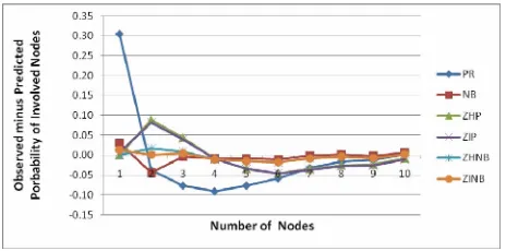
The minimum BIC was observed for the NB model, fol-lowed by ZHNB/ZINB models. However, other validity indices of the model (maximum log likelihood, mini-mum AIC, MSPE and MAPE) favored ZHNB/ZINB models over all other models. The plot of observed mi-nus predicted probability of involved nodes at each count is shown in Figure 1. The PR model
underesti-mates probability of occurrence of negative node and overestimates occurrence of one positive node. The line of difference between observed minus predicted prob-ability of positive nodes was close to the reference zero line, showing better fit of ZHNB/ZINB models than the other models. There is virtually no difference between ZHNB and ZINB models in all aspects of describing the number of involved nodes. The ZINB model provides
[image:7.595.309.541.441.556.2]slightly smaller validity indices as compared to ZHNB. Finally, the ZINB model was assessed by the leave one out cross validation method. The MSPE in cross valida-tion of the ZINB model was the lowest of all the models (0.0007), indicating that the ZINB model performs well for predicting nodal involvement in future patients. The ZINB model predicts that 70.6% all negative nodes are at “low risk” zeros, and the remaining 29.4% are at “high risk” for negative nodes. This indicates that almost 30% of the patients observed as negative for nodal in-volvement are at “high risk” of nodal inin-volvement based on cofactors.
Table 1 displays the estimates of regression
coeffi-cients for various cofactors of both portions of the ZINB model. For ZINB, the results of both parts of the models together help in understanding the role of the factors on nodal distribution. The logistic portion showed that me-dial primary site and absence of skin changes signifi-cantly increased the chance of negative nodes in breast cancer patients. Negative binomial portion reveals that the risk of a greater number of involved nodes was 82 percent higher in single/doubleparous patients versus nulliparous patients, given that the patients are in a high- risk group. Further, this was 95 percent higher among multiparous patients. The patients with lateral site in-volvement had 1.29 times higher likelihood for having a larger number of positive nodes than patients with the medial site. Women with skin changes had 1.39 times more involvement of higher positive nodes as compared
[image:7.595.57.539.618.722.2]Figure 1. Plots of observed minus predicted probability of positive nodes versus number of positive nodes for six models.
Table 2. Comparison of model fit characteristics.
PR NB ZHP ZIP ZHNB ZINB
Log Likelihood –4093.9 –2598.6 –3019.7 –3018.4 –2553.7 –2551.1
AIC 8221.8 5233.1 6107.4 6104.8 5185.4 5172.2
BIC 8307.6 5324.0 6279.0 6276.5 5382.3 5348.9
MSPE 4764.0 139.1 632.5 627.62 52.9 49.2
Copyright © 2010 SciRes. Openly accessible at http://www.scirp.org/journal/HEALTH/
to their counterparts. The chance of increased positive nodes was 28 percent higher among patients with 2-5 cm tumor size, in comparison to patients with less than 2 cm tumor size. It was again 1.49 times more likely among patients with more than 5 cm tumor size as compared to less than 2 cm tumor size.
4. DISCUSSION
The number of involved nodes is one of the most impor-tant therapeutic and prognostic factors for breast cancer [1]. Clinicians need to predict the number of involved nodes in breast cancer patients in order to improve health outcomes. To the best of our knowledge, few studies have described the number of involved nodes in breast cancer patients, and tested statistical models to accu-rately predict involved node number. As for most of the count data, studies also found excess variability in nodal distribution than that expected by a Poisson model. They also generally assume the cause of over-dispersion to be solely due to unobserved heterogeneity, and therefore used the NB model to fit and describe nodal frequency [3,4]. However, data with nodal involvement often in-volve excess zeros, which also cause over-dispersion. This indicates a need to explore fitting zero hurdle and zero inflated models, which can also account for vari-ability due to excessive zeros. In the current paper, we fitted various count models to identify putative causes of over-dispersion, and to assess the predictive performance of these models with regard to the nodal status in a population of patients with breast cancer. We also illus-trated the significance of using zero inflated models in count data involving zeros that emanate from the sub-jects that are all “at-risk” of the event of interest.
The ZHNB/ZINB regression models provide the best fit when predicting the number of involved nodes in breast cancer patients. This confirms that the distribution of the involved nodes contained over-dispersion not only due to unobserved heterogeneity but also due to exces-sive negative nodes (zeros). As expected, the PR model had the worst prediction ability for nodal frequency. Accounting only one source of over-dispersion, either due to excessive zeros or due to unobserved heterogene-ity, the prediction ability of nodal frequency improved as indicated by NB, ZHP, ZIP models. However, use of ZHNB/ZINB models, which assumes involvement of more than just one source of over-dispersion, provided smaller prediction error.
The ZHNB and ZINB models were consistent and similar for factor-identification in the extent of nodal involvement as well as for prediction of number of posi-tive (involved) nodes. In the current study, we focused on predicting nodal frequency. On that basis, either model
can be used to predict number of involved nodes. Due to ease of interpreting the results of ZHNB model, it can be preferred over ZINB model. These findings are sup-ported by Rose et al.[6], who also found good
concor-dance between the ZHNB and ZINB models on vaccine adverse data—a case of only “at risk” zeros similar to the data used in our study. They suggested that the model selection should be determined based on study objec-tives and the data generating process. They recommend using the ZHNB model due to involvement of only “at risk” zeros. However, Baughman [31] suggested that model choice should be based on the rationale behind the consideration of data generating mechanism. Gilt-horpe et al. [32] suggested that the zero inflated models
should be used according to the underlying disease process i.e., considerations of disease onset and disease
progression. In our opinion, zero hurdle models should be preferred if data consist of zeros which are all coming from the subjects at “no-risk” of the outcome of interest, and over-dispersion is due to excess zeros. In such cases, zeros from the “no-risk” population arise from a non- counting process. However, zeros coming from an “at risk” population belong to the count process, thus influ-encing model choice based on the rationale behind the data generation of the “at risk” population. In the present study, if diagnosis is close to or at disease onset, the risk of finding the event of interest (nodal involvement) would be minimal, whereas if the diagnosis is late and during disease progression, the risk of the event of inter-est would be relatively high. Previous studies note that the distribution of involved nodes often consists of some proportion of false negative nodes, which may often arise in the “high-risk” group [7,8]. There is ample evi-dence to consider “at risk” zeros, at least in breast cancer, as a mixture of “low-risk” and “high-risk” zeros, thus, suggesting the use of zero inflated models. Use of the ZINB model not only gives estimate of the false nega-tive nodes i.e., zero at “high risk” of nodal involvement,
but also provides slightly better predictive performance than the ZHNB model.
The mean square prediction error was found to be 35.4% less using ZINB as compared to the NB regres-sion model. In addition, the predictive performance of the ZINB model was significantly better than the NB regression model, indicating that the NB model may not always be appropriate for describing nodal distribution. The leave-one-out cross-validation assessment of the developed ZINB model provided the minimum mean square prediction error compared to the other developed models, indicating that the model performs well, even for future patients, in comparison to other models.
This study is the first report to analyze patterns of nodal involvement in breast cancer, using a large dataset collected in India. In our study, 61.2% of the patients had the presence of involved nodes. Sandhu et al.,using
a different Indian dataset, also reported a 61.6% nodal involvement [33]. A different study, also using a popula-tion from India, reported an even higher nodal positivity rate of 80.2% [34]. In our study, both presence of other than medial primary site and skin changes among pa-tients are associated with high risk of nodal involvement and with a greater number of involved nodes. In addition to these two factors, higher parity and larger tumor size are also associated with an increased risk of a higher number of involved nodes, given that the patients are in high risk population. These factors are consistently found to be associated with the presence of involved nodes in other studies [35-41], and are directly or indirectly sequences of late diagnosis. Overall, these findings con-firm the need for ongoing efforts to minimize diagnostic delay in patients suspected of having breast cancer.
One limitation to our study is that it uses a dataset not designed for our analysis. Important covariates, such as lymphatic vascular invasion and S-phase function, were not included in this database. These covariates could be significantly associated with involved nodes, as reported in various studies [42-45]. In addition, instead of ad-justment of these results in relation to dissected number of nodes, an attempt could be made to model the propor-tion of positive nodes in patients through count data models or binomial models.
5. CONCLUSIONS
The ZHNB/ZINB regression models can be used to de-scribe nodal distribution more appropriately than the NB model. However, the ability of the ZINB model to more accurately estimate at “high-risk” zeros while having a comparatively lower prediction error, as compared to the ZHNB model, suggests that it is the best model for pre-dicting and describing the number of involved nodes. Many of the factors associated with nodal involvement may be a result of diagnostic delay of breast cancer
pa-tients, indicating the need to minimize delay in diagnosis of breast cancer patients. There is also a need to further investigate the consequences of using zero inflated mod-els, as an alternative to zero hurdle modmod-els, in at- risk populations.
6. ACKNOWLEDGEMENTS
The authors would like to express their thanks to Dr. V. Sreenivas, Department of Biostatistics, All India Institute of Medical Sciences, New Delhi; Dr. Arvind Pandey, National Institute of Medical Statistics, New Delhi; and also Dr. Kishore Chaudhry and Dr. D. K. Shukla, Division of Non-Communicable Diseases, Indian Council of Medical Research, New Delhi, for their critical comments throughout this study.
REFERENCES
[1] Hernandez-Avila, C.A., Song, C., Kuo, L., Tennen, H., Armeli, S. and Kranzler, H.R. (2006) Targeted versus daily naltrexone: Secondary analysis of effects on aver-age daily drinking. Alcoholism, Clinical and Experimen-tal Research, 30(5), 860-865.
[2] Slymen, D.J., Ayala, G.X., Arredondo, E.M. and Elder, J.P. (2006) A demonstration of modeling count data with an application to physical activity. Epidemiologic Per-spectives & Innovations, 3(3), 1-9.
[3] Horton, N.J., Kim, E. and Saitz, R. (2007) A cautionary note regarding count models of alcohol consumption in randomized controlled trials. BioMed Central Medical Research Methodology, 7(9), 1-9.
[4] Salinas-Rodriguez, A., Manrique-Espinoza, B. and Sosa- Rubi, S.G. (2009) Statistical analysis for count data: Use of health services applications. Salud Publica Mex, 51(5), 397-406.
[5] Asada, Y. and Kephart, G. (2007)Equity in health ser-vices use and intensity of use in Canada. Biomed Central Health Services Research, 7(41), 1-12.
[6] Grootendorst, P.V. (1995) A comparison of alternative models of prescription drug utilization. Health Econom-ics, 4(3), 183-198.
[7] Afifi, A.A., Kotlerman, J.B., Ettner, S.L. and Cowan, M. (2007) Methods for improving regression analysis for skewed continuous or counted responses. Annual Review of Public Health, 28, 95-111.
[8] Hur, K., Hedeker, D., Henderson, W., Khuri, S. and Daley, J. (2002) Modeling clustered count data with ex-cess zeros in health care outcomes research. Health Ser-vices and Outcomes Research Methodology, 2002, 3, 5-20.
[9] Lee, A.H., Wang, K., Scott, J.A., Yau, K.K. and McLach-lan, G.J. (2006) Multi-level zero-inflated Poisson regres-sion modeling of correlated count data with excess zeros.
Statistical Methods in Medical Research, 15(1),47-61.
[10] Yau, K.K. and Lee, A.H. (2001) Zero-inflated Poisson regression with random effects to evaluate an occupa-tional injury prevention programme. Statistics in Medi-cine, 20 (19), 2907-2920.
Copyright © 2010 SciRes. Openly accessible at http://www.scirp.org/journal/HEALTH/ repeated measures of zero-inflated count data. Statistical
Modelling, 5(1), 1-19.
[12] Gardner, W., Mulvey, E.P. and Shaw, E.C. (1995) Re-gression analyses of counts and rates: Poisson, overdis-persed Poisson, and negative binomial models. Psycho-logical Bulletin, 118(3),392-404.
[13] Hardin, J.W. and Hilbe, J.M. (2007) Generalized Linear Models and Extensions. A Stata Press Publication, Stat-Corp LP, Texas.
[14] Mullay, J. (1986) Specifications and testing of some modified count data model. Journal of Econometrics,
33(3), 341-365.
[15] Lambert, D. (1992) Zero-inflated Poisson regression, with application to defects in manufacturing. Technomet-rics, 34(1),1-14.
[16] Vuong, Q.H. (1989) Likelihood ratio tests for model selection and non-nested hypotheses. Econometrica, 57 (2), 307-333.
[17] Picard, R. and Cook, D. (1984) Cross-Validation of Re-gression Models. Journal of the American Statistical As-sociation, 79(387), 575-583.
[18] Baughman, L.A. (2007) Mixture model framework fa-cilitates understanding of zero-inflated and hurdle mod-els for count data. Journal of Biopharmaceutical Statis-tics, 17(5), 943-946.
[19] Gilthorpe, M.S., Frydenberg, M., Cheng, Y. and Baelum, V. (2009) Modelling count data with excessive zeros: The need for class prediction in zero-inflated models and the issue of data generation in choosing between zero-in-flated and generic mixture models for dental caries data.
Statistics in Medicine, 28(28), 3539-3553.
[20] Sandhu, D.S., Sandhu, S., Karwasra, R.K. and Marwah, S. (2010) Profile of breast cancer patients at a tertiary care hospital in north India. Indian Journal of Cancer,
47(1), 16-22.
[21] Saxena, S., Rekhi, B., Bansal, A., Bagga, A., Chintamani and Murthy, N.S. (2005) Clinico-morphological patterns of breast cancer including family history in a New Delhi hospital, India-A cross-sectional study. World Journal of Surgical Oncology, 3, 67-75.
[22] Nouh, M.A., Ismail, H., Ali El-Din, N.H. and El-Bol-kainy, M.N. (2004) Lymph node metastasis in breast car-cinoma: Clinicopathologic correlations in 3747 patients.
Journal of Egyptian National Cancer Institute, 16(1),
50-56.
[23] Gann, P.H., Colilla, S.A., Gapstur, S.M., Winchester, D.J. and Winchester, D.P. (1999) Factors associated with axil-lary lymph node metastasis from breast carcinoma de-scriptive and predictive analyses. Cancer, 86(8), 1511-
1518.
[24] Olivotto, I.A., Jackson, J.S.H., Mates, D., Andersen, S., Davidson, W., Bryce, C.J. and Ragaz, J. (1998) Predic-tion of axillary lymph node involvement of women with invasive breast carcinoma a multivariate analysis. Cancer,
83(5), 948-955.
[25] Ravdin, P.M., De Laurentiis, M., Vendely, T. and Clark, G.M. (1994) Prediction of axillary lymph node status in breast cancer patients by use of prognostic indicators.
Journal of National Cancer Institute, 86(23), 1771-1775.
[26] Chua, B., Ung, O., Taylor, R. and Boyages, J. (2001) Fre- quency and predictors of axillary lymph node metastases in invasive breast cancer. Australian and New Zealand
Journal of Surgery, 71(12), 723-728.
[27] Manjer, J., Balldina, G. and Garne, J.P. (2004) Tumour location and axillary lymph node involvement in breast cancer: A series of 3472 cases from Sweden. European
Journal of Surgical Oncology, 30(6), 610-617.
[28] Manjer, J., Balldin, G., Zackrisson, S. and Garne, J.P. (2005) Parity in relation to risk of axillary lymph node involvement in women with breast cancer. European Surgical Research, 37(3),179-184.
[29] Olivotto, I.A., Jackson, J.S.H., Mates, D., Andersen, S., Davidson, W., Bryce, C.J. and Ragaz, J. (1998) Predic-tion of axillary lymph node involvement of women with invasive breast carcinoma a multivariate analysis. Cancer,
83(5), 948-955.
[30] Ravdin, P.M., De Laurentiis, M., Vendely, T. and Clark, G.M. (1994) Prediction of axillary lymph node status in breast cancer patients by use of prognostic indicators.
Journal of National Cancer Institute, 86(23), 1771-1775.
[31] Chua, B., Ung, O., Taylor, R. and Boyages, J. (2001) Frequency and predictors of axillary lymph node metas-tases in invasive breast cancer. Australian and New Zea-land Journal of Surgery, 71(12), 723-728.
[32] Cetintas, S.K., Kurt, M., Ozkan, L., Engin, K., Gokgoz, S. and Tasdelen, I. (2006) Factors influencing axillary node metastasis in breast cancer. Tumori, 92(5), 416-422. [33] Fisher, B., Bauer, M., Wickerham, D.L., Redmond,
C.L.K. and Fisher, E.R. (1983) Relation of number of positive axillary nodes to the prognosis of patients with primary breast cancer. Cancer, 52(9), 1551-1557. [34] Harden, S.P., Neal, A.J., Al-Nasiri, N., Ashley, S. and
Quercidella, R.G. (2001) Predicting axillary lymph node metastases in patients with T1 infiltrating ductal carci-noma of the breast. The Breast, 10(2), 155-159.
[35] Guern, A.S. and Vinh-Hung, V. (2008) Statistical distri-bution of involved axillary lymph nodes in breast cancer.
Bull Cancer, 95(4), 449-455.
[36] Kendal, W.S. (2005) Statistical kinematics of axillary nodal metastases in breast carcinoma. Clinical & Expe- rimental Metastasis, 22(2), 177-183.
[37] Cameron, A.C. and Trivedi, P.K. (1998) Regression Analysis of Count Data. Econometric Society Mono-graph, Cambridge University Press, New York.
[38] Rose, C.E., Martin, S.W., Wannemuehler, K.A. and Plikaytis, B.D. (2006) On the use of zero-inflated and hurdle models for modeling vaccine adverse event count data. Journal of Biopharmaceutical Statistics, 16(4),
463-481.
[39] Rampaul, R.S., Miremadi, A., Pinder, S.E., Lee, A. and Ellis, I.O. (2001) Pathological validation and significance of micrometastasis in sentinel nodes in primary breast cancer. Breast Cancer Research, 3(2), 113-116.
[40] Schaapveld. M., Otter, R., de Vries, E.G., Fidler, V., Grond, J.A., van der Graaf, W.T., de Vogel, P.L. and Will- emse, P.H. (2004) Variability in axillary lymph node dis-section for breast cancer. Journal of Surgical Oncology,
87(1), 4-12.
[41] Martin, T.G., Wintle, B.A., Rhodes, J.R., Kuhnert, P.M., Field, S.A., Low-Choy, S.J., Tyre, A.J. and Possingham, H.P. (2005) Zero tolerance ecology: Improving ecologi-cal inference by modeling the source of zero observa-tions. Ecology Letters, 8(11), 1235-1246.
Poisson specifications. Midwest Political Science Assoc- iation, San Diego.
[43] Boucher, J.P., Denuit, M. and Guillen, M. (2007) Risk classification for claim counts: A comparative analysis of various zero inflated mixed Poisson and hurdle models.
North American Actuarial Journal, 11(4),110-131. [44] Bohning, D., Dietz, E., Schlattmann, P., Mendonca, L.
and Kirchner, U. (1999) The zero inflated Poisson model and the decayed, missing and filled teeth index in dental epidemiology. Journal of the Royal Statistical Society
(Series A), 162(2),195-209.